1/24kongr7_e.doc

12. Measurement of Low Frequency Electrical and MagneticFields

EMF Congress - March 29, 1995

Speaker: Dietmar TandlerWandel & Goltermann GmbH & Co

Tel. +49-7121-86-1523

Contents

1 Introduction........................................................................................................................ 22 The origin of low-frequency electromagnetic fields ......................................................... 2

2.1 Electrical fields .................................................................................................... 32.2 Magnetic fields..................................................................................................... 42.3 Electrical and magnetic equivalent field strength................................................ 72.4 Field generators and order of magnitude of field strengths ................................. 9

3 Measurement techniques and errors .................................................................................. 133.1 Technique for measuring magnetic fields............................................................ 143.2 Technique for measuring electrical fields............................................................ 17

4 W&G's line of equipment for measuring low-frequency electromagnetic fields.............. 224.1 Development criteria............................................................................................ 224.2 Overall concept.................................................................................................... 234.3 Specifications for the basic device....................................................................... 254.4 Operation and applications of the devices ........................................................... 264.5 Device calibration................................................................................................ 29

5 The EFA-1, EFA-2 and EFA-3 device versions ................................................................ 306 Bibliography ...................................................................................................................... 30

1 Introduction

In the past, the question of whether high-frequency electromagnetic fields affect biological organisms and, if so,how, has gained increasing attention. The focus became sharper as high-frequency generators such as microwaveovens have become popular. In recent times concerns have grown that the increasing number of transmitters (e.g.cellular radio, radar) might have some effect on the health of the populace at large. It is in this context that low-frequency electrical and magnetic fields have been the subject of more intensive discussion. The suspicion thatmagnetic fields generated by long-distance power lines, for example, might be responsible for various medicalsymptoms has encited heat discussion among different committees.This paper will not consider the question of whether such low-frequency fields affect organisms and if so, how.Instead, test equipment for measuring such fields will be described. Current literature has much to say about thephysics of these fields. However, the various approaches come up short when it is time to measure the fieldparameters with some degree of precision. Accordingly, this paper will examine the possible measurement errors andshortcomings of field sensors based on the underlying theory of electromagnetic fields, thereby allowing a criticalchoice among the measuring devices currently available commercially.Wandel & Goltermann is introducing a new line of measuring devices which were developed especially forrecording low-frequency electrical and magnetic fields. The concept of these devices will be presented inconjunction with the theoretical considerations.

2 The origin of low-frequency electromagnetic fields

What do low-frequency fields look like, how do they arise and on what order of magnitude is their field strength?Unlike static fields, alternating electromagnetic fields arise whenever (alternating) current flows through a conductor,i.e. whenever charge is brought into motion. A magnetic field always arises alongside of the electrical field.Electrical and magnetic fields of equal power also behave according to the relationship between current intensity andvoltage:A high voltage produces a relatively strong electrical field with a relatively weak magnetic field, and vice versa.During the last century (1873) the English physician James Clerk Maxwell developed a closed system of equationsfor mathematically describing electromagnetic fields. Reference will be made to these equations later in this paper.His theories are useful in explaining many relationships in field theory.

2.1 Electrical fields

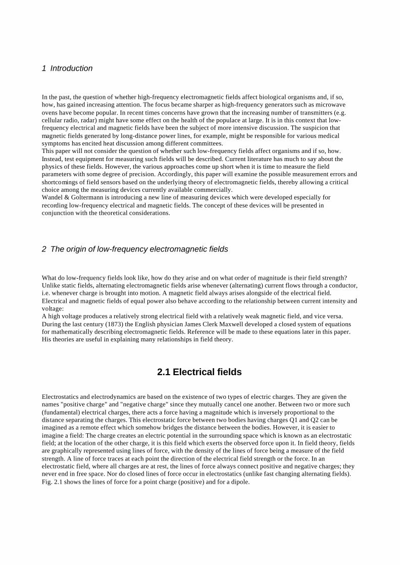
Electrostatics and electrodynamics are based on the existence of two types of electric charges. They are given thenames "positive charge" and "negative charge" since they mutually cancel one another. Between two or more such(fundamental) electrical charges, there acts a force having a magnitude which is inversely proportional to thedistance separating the charges. This electrostatic force between two bodies having charges Q1 and Q2 can beimagined as a remote effect which somehow bridges the distance between the bodies. However, it is easier toimagine a field: The charge creates an electric potential in the surrounding space which is known as an electrostaticfield; at the location of the other charge, it is this field which exerts the observed force upon it. In field theory, fieldsare graphically represented using lines of force, with the density of the lines of force being a measure of the fieldstrength. A line of force traces at each point the direction of the electrical field strength or the force. In anelectrostatic field, where all charges are at rest, the lines of force always connect positive and negative charges; theynever end in free space. Nor do closed lines of force occur in electrostatics (unlike fast changing alternating fields).Fig. 2.1 shows the lines of force for a point charge (positive) and for a dipole.

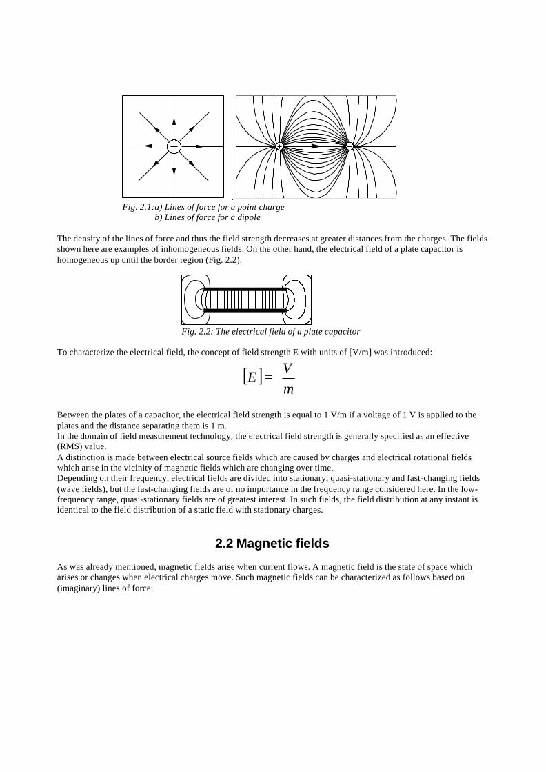
Fig. 2.1:a) Lines of force for a point chargeb) Lines of force for a dipole

The density of the lines of force and thus the field strength decreases at greater distances from the charges. The fieldsshown here are examples of inhomogeneous fields. On the other hand, the electrical field of a plate capacitor ishomogeneous up until the border region (Fig. 2.2).

Fig. 2.2: The electrical field of a plate capacitor

To characterize the electrical field, the concept of field strength E with units of [V/m] was introduced:

[ ]

=mV

E

Between the plates of a capacitor, the electrical field strength is equal to 1 V/m if a voltage of 1 V is applied to theplates and the distance separating them is 1 m.In the domain of field measurement technology, the electrical field strength is generally specified as an effective(RMS) value.A distinction is made between electrical source fields which are caused by charges and electrical rotational fieldswhich arise in the vicinity of magnetic fields which are changing over time.Depending on their frequency, electrical fields are divided into stationary, quasi-stationary and fast-changing fields(wave fields), but the fast-changing fields are of no importance in the frequency range considered here. In the low-frequency range, quasi-stationary fields are of greatest interest. In such fields, the field distribution at any instant isidentical to the field distribution of a static field with stationary charges.

2.2 Magnetic fields

As was already mentioned, magnetic fields arise when current flows. A magnetic field is the state of space whicharises or changes when electrical charges move. Such magnetic fields can be characterized as follows based on(imaginary) lines of force:

4/24kongr7_e.doc

I

r

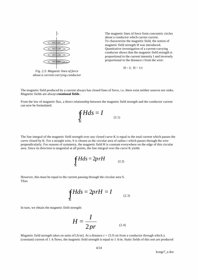
Fig. 2.3: Magnetic lines of forceabout a current-carrying conductor

The magnetic lines of force form concentric circlesabout a conductor which carries current.To characterize the magnetic field, the notion ofmagnetic field strength H was introduced.Quantitative investigation of a current-carryingconductor shows that the magnetic field strength isproportional to the current intensity I and inverselyproportional to the distance r from the wire:

H ~ I; H ~ 1/r

The magnetic field produced by a current always has closed lines of force, i.e. there exist neither sources nor sinks.Magnetic fields are always rotational fields .

From the law of magnetic flux, a direct relationship between the magnetic field strength and the conductor currentcan now be formulated:

∫ =K

IHds (2.1)

The line integral of the magnetic field strength over any closed curve K is equal to the total current which passes thecurve closed by K. For a straight wire, S is chosen as the circular area of radius r which passes through the wireperpendicularly. For reasons of symmetry, the magnetic field H is constant everywhere on the edge of this circulararea. Since its direction is tangential at all points, the line integral over the curve K yields

∫ =K

rHHds π2 (2.2)

However, this must be equal to the current passing through the circular area S.Thus

∫ ==K

IrHHds π2 (2.3)

In turn, we obtain the magnetic field strength:

HI

r=

2π (2.4)

Magnetic field strength takes on units of [A/m]. At a distance r = 15.9 cm from a conductor through which a(constant) current of 1 A flows, the magnetic field strength is equal to 1 A/m. Static fields of this sort are produced

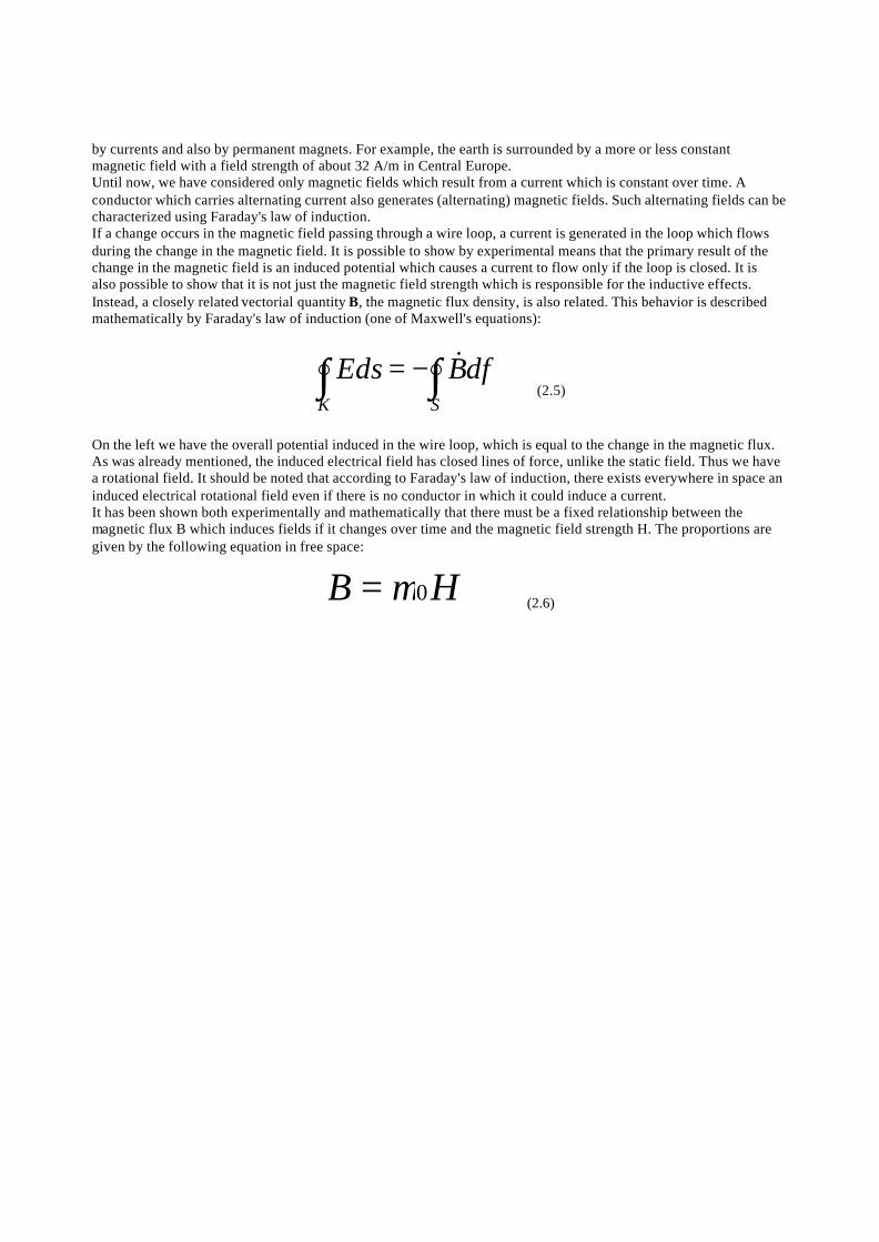
by currents and also by permanent magnets. For example, the earth is surrounded by a more or less constantmagnetic field with a field strength of about 32 A/m in Central Europe.Until now, we have considered only magnetic fields which result from a current which is constant over time. Aconductor which carries alternating current also generates (alternating) magnetic fields. Such alternating fields can becharacterized using Faraday's law of induction.If a change occurs in the magnetic field passing through a wire loop, a current is generated in the loop which flowsduring the change in the magnetic field. It is possible to show by experimental means that the primary result of thechange in the magnetic field is an induced potential which causes a current to flow only if the loop is closed. It isalso possible to show that it is not just the magnetic field strength which is responsible for the inductive effects.Instead, a closely related vectorial quantity B, the magnetic flux density, is also related. This behavior is describedmathematically by Faraday's law of induction (one of Maxwell's equations):

∫ ∫−=K S

dfBEds & (2.5)

On the left we have the overall potential induced in the wire loop, which is equal to the change in the magnetic flux.As was already mentioned, the induced electrical field has closed lines of force, unlike the static field. Thus we havea rotational field. It should be noted that according to Faraday's law of induction, there exists everywhere in space aninduced electrical rotational field even if there is no conductor in which it could induce a current.It has been shown both experimentally and mathematically that there must be a fixed relationship between themagnetic flux B which induces fields if it changes over time and the magnetic field strength H. The proportions aregiven by the following equation in free space:

B H= µ0 (2.6)

µ0 is the permeability of free space or the magnetic field constant. Its magnitude and dimensions are as follows:

µ0 1 256 6= −. EVsAm

It is common to use the magnetic flux density B instead of the magnetic field strength H as a measure of the strengthof a magnetic field. The unit of magnetic flux density is the [T] (Tesla) or Gauss (in the US; 1 G = 100 µT).The above equation holds only in free space. Otherwise, a material-dependent coefficient must be taken into account:

B Hr= µ µ0

For air, the relative permeability is about 1. We thus obtain:

1 1 257Am

T≈ . µ

2.3 Electrical and magnetic equivalent field strength

Until now, we have looked at basic examples illustrating the origin of electromagnetic fields. These were two-dimensional representations of field curves. However, the electrical and magnetic fields are vectorial fields, i.e. theyhave a specific magnitude and direction at every point in space. These factors are a function of time in quasi-stationary fields. To investigate a field at a certain point, it is useful to measure all three orthogonal components bymagnitude and phase (vs. time). In personal safety applications (one usage of field measuring devices), such preciseanalysis of the fields is unnecessary, however. It suffices to determine a field strength figure which provides enoughinformation to know whether persons are endangered or not. Accordingly, the notion of equivalent field strengthwas defined for electrical and magnetic fields (VDE 0848 Part 1):

Z

X

Y

Ex

Ey

EzEe

Fig. 2.4: Vectorial components

of the electrical field strength

E E E Ee x y z= + +2 2 2

H H H He x y z= + +2 2 2 (2.8)

The equivalent field strength consists of the quadratic average of the three field components; the phasediffe rences between the three components do not enter into this parameter.

Neglecting the phase information does have consequences when it comes to a precise characterization of thefield. Due to the "near-field" measurement - fields borne by conductors (low-frequency fields) are near fields -the varying phase differences vs. time must be taken into account; the peak of the field vector forms an ellipse inspace, whence the term elliptically polarized field. If the field strength vector does not change directions (due tofield components of the same phase), the term used is linear polarization. In this special case, the equivalent fieldstrength Ee (or He) is equal to the magnitude of the field strength E (or H). In a linearly polarized field, the

position of a field probe is of no consequence as long as it correctly breaks down the field into its threeorthogonal components. Since in this case the equivalent field strength Ee (or He) is equal to the magnitude ofthe field strength E (or H), this sensor will always measure the correct field strength E (or H). By forming thequadratic average from the three field components, such a sensor has ideal isotropy for linear polarization. Thesubject of isotropy will be considered later in greater detail in relation to the E-field sensor.When such a sensor is used in an elliptically polarized field, the results it provides are too high (due to theneglected phase relationships). In principle, the worst-case field strength is measured, which is allowable forpersonal safety applications.

2.4 Field generators and order of magnitude of field strengths

Just where do such fields occur and at what intensity levels? Obvious examples of intense 50 Hz fields areenergy transmission systems (such as long-distance power lines and transformers) and devices which consumeenergy (such as electrical machinery of all sorts).

((Bildtext:))400 Hz on-board power supplyPower plantTransformerPower grid 220/380 kVHeavy industryRailwaysPrivate homesBusiness, industry, offices, storesAgricultureSmall plants

TransformatorVerbundnetz220/380 kV

Gewerbe, Industrie,Büro- und Warenhäuser

20 kV

Großindustrie

110/220 kV

20 kV

Wohnhäuser

220/ 380 V

110 kV

20 kV

220/380 V 220/380 V

L andwir tschaft Kleinbetriebe

Schi nenverkehr

Kraf twerk

400 Hz Bordstromversorgung

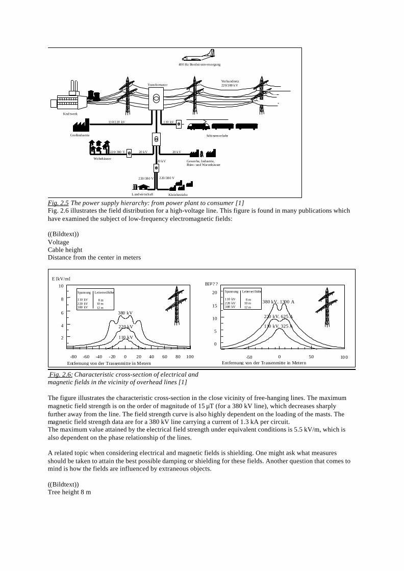
Fig. 2.5 The power supply hierarchy: from power plant to consumer [1]Fig. 2.6 illustrates the field distribution for a high-voltage line. This figure is found in many publications whichhave examined the subject of low-frequency electromagnetic fields:

((Bildtext))VoltageCable heightDistance from the center in meters

-50 0 50 10 0

0

5

10

15

20

-80 -60 -40 -20 0 20 40 60 80 100

10

8

6

4

2

Spannung Leiterseilhöhe

110 kV220 kV380 kV

8 m10 m12 m

380 kV

220 kV

110 kV

Spannung Leiter sei lhöhe

110 kV220 kV380 kV

8 m10 m12 m

380 kV, 1300 A

220 kV, 625 A

110 kV, 325 A

Entfernung von der Trassenmitte in Metern

E [kV/m]

Entfernung von der Trassenmitte in Metern

B[µ? ?

Fig. 2.6: Characteristic cross-section of electrical andmagnetic fields in the vicinity of overhead lines [1]

The figure illustrates the characteristic cross-section in the close vicinity of free-hanging lines. The maximummagnetic field strength is on the order of magnitude of 15 µT (for a 380 kV line), which decreases sharplyfurther away from the line. The field strength curve is also highly dependent on the loading of the masts. Themagnetic field strength data are for a 380 kV line carrying a current of 1.3 kA per circuit.The maximum value attained by the electrical field strength under equivalent conditions is 5.5 kV/m, which isalso dependent on the phase relationship of the lines.

A related topic when considering electrical and magnetic fields is shielding. One might ask what measuresshould be taken to attain the best possible damping or shielding for these fields. Another question that comes tomind is how the fields are influenced by extraneous objects.

((Bildtext))Tree height 8 m

Unlike magnetic fields, the electrical field can be easily influenced and shielded using conductive materials.Fig. 2.7: Influence of a tree on the electrical field in the immediate vicinity of an overhead line [1]

05 m

10 m15 m

20 m

100 %

E

75 %

15 %

Baumhöhe8 m

A tree reduces the electrical field of a 380 kV line up to 15% in its immediate vicinity. However, the shieldingeffect decreases at greater distances. As will be seen later, the shielding effect of objects with respect to theelectrical field causes problems when measuring fields since the presence of a person during a measurement willdistort the field.A list of the different field strengths which occur in the LF range is perhaps relevant at this point:

Electrical field in[V/m]

Source Magnetic field in[µT]

Source

15000 380 kV station

10000 380 kV line 2500 Hairdryer

3000 110 kV line 1000 Electric range

500 10 kV line 500 Television

>10000 Human-bornefields

50 380 kV line

5 - 40 Electricalinstallation

20 110 kV line

300 Fluorescent light 15 Electric space heater

300 - 700 Television 10 Desktop lamp

30 Subway (nearground)

6 10 kV line

2 220 V installation

Magnetic field strengths range from a few nT (approx. 50 to 70 nT in the home with appliances switched off) toapprox. 1 to 2 mT. Electrical field strengths range from a few V/m to several 10 kV/m.

One could easily continue this list. In our case, however, it is intended as an overview of real-world fieldstrengths which are relevant to later observations. The main interest is in the area of "personal safety", which isthe subject of much discussion at this time. Unlike high-frequency fields, effects of low-frequency fields onbiological mechanisms are either difficult or impossible to verify. The heating which occurs in organic materialexposed to high-frequency fields does not occur with (strong) low-frequency fields. Many published studies haverecounted extensive experiments involving animals and humans as well as epidemiological investigations (theoccurrence of diseases in the human population was studied with the aim of establishing a correlation between adisease and one or more related factors). For example, test persons were subjected to magnetic fields on theorder of magnitude of 5 mT at a frequency of 50 Hz. As with many other studies, the results were not clear. Itwas not possible to establish clear damages or impairments of these test persons in comparison with other groupsof persons who were not subjected to any fields. On the other hand, increased incidences of leukemia are beinginvestigated which - as some have maintained - were provoked by high-voltage lines situated in the vicinity ofresidences. One difficulty of retrospective studies of this sort is the problem of considering a group of diseasevictims as representative since comparisons with other (endangered) groups of persons are meaningful only if the"environmental parameters" agree.Given the fact that about 12,000 published articles have not reached a clear consensus, we will restrict ourselvesto stating the limits which various committees have proposed in the form of recommendations or legaldocuments. Such limits are intended to protect persons subjected to continuous exposure from possible negativeconsequences. The limits are defined with respect to frequency (from 0 Hz to 30 kHz) and differ in their coursedepending on the committee. The limits for continuous exposure to a 50 Hz magnetic field are as follows:

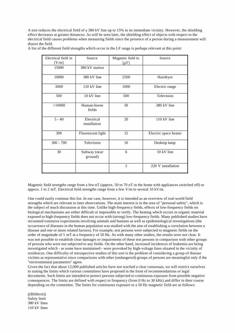
((Bildtext))Safety limit380 kV lines110 kV lines

Limits for pacemakersLimits for ventricular fibrillationsDomestic appliancesMagnetic flux density

Fig. 2.8 Limits for continuousexposure to a 50 Hz magnetic field[1]

From these figures, one canconclude that test equipment should

be able to measure in the range from several 10 nT to 10 mT (magnetic field; 5 mT upper threshold) and several10 V/m to 20 kV/m (as stipulated by the DKE = German Electrical Engineering Commission).According to the IRPA, the maximum values for continuous exposure of persons are 5 kV/m (electrical field)and 100 µT (magnetic field).The actual limits which become accepted in the future are inconsequential for the test and measurement industryas long as the test equipment covers the related field strengths (ranges) with the specified accuracy and uses theprescribed measurement technique(s).

3 Measurement techniques and errors

Based on knowledge of theoretical physics as it concerns electromagnetic fields, measurement techniques (i.e.sensors) can be developed to handle the field parameters. This section will take a closer look at the measurementtechniques which provide the best results given the current state of the art. Various problem areas will also beconsidered which, either for theoretical reasons or due to incorrect handling of the field measuring devices, canlead to measurement errors.

3.1 Technique for measuring magnetic fields

A commonly used method for measuring magnetic fields involves a practical implementation of Faraday's law ofinduction. Here, the fact that alternating magnetic fields induce a voltage in a coil which is proportional to thefield strength is exploited.

A magnetic field which passes vertically through the coil induces the following voltage in the coil:

U n fBAind = 2π Eq. 3.1

n : Number of turnsf : FrequencyB : Magnetic inductionA : Cross-sectional area of the coil

If the coil has a high-impedance termination, the field strength can be determined directly by measuring theinduced voltage:

0,01 0,1 1 10 100 1000 10000 100000 1 MIO

WHO / IRPA 100 µT

VDE 0848 400 µT

Sicherheitsgrenzw ert5000 µT

380 kV Leitungen

110 kV Leitungen

Haushaltsgerä te

magnetische Flußdichte ( µT)

Störschwellen für Herzschrittmacher

Schwellen für Herzkammerflimmern

BU

n fAind=

2π Eq. 3.2

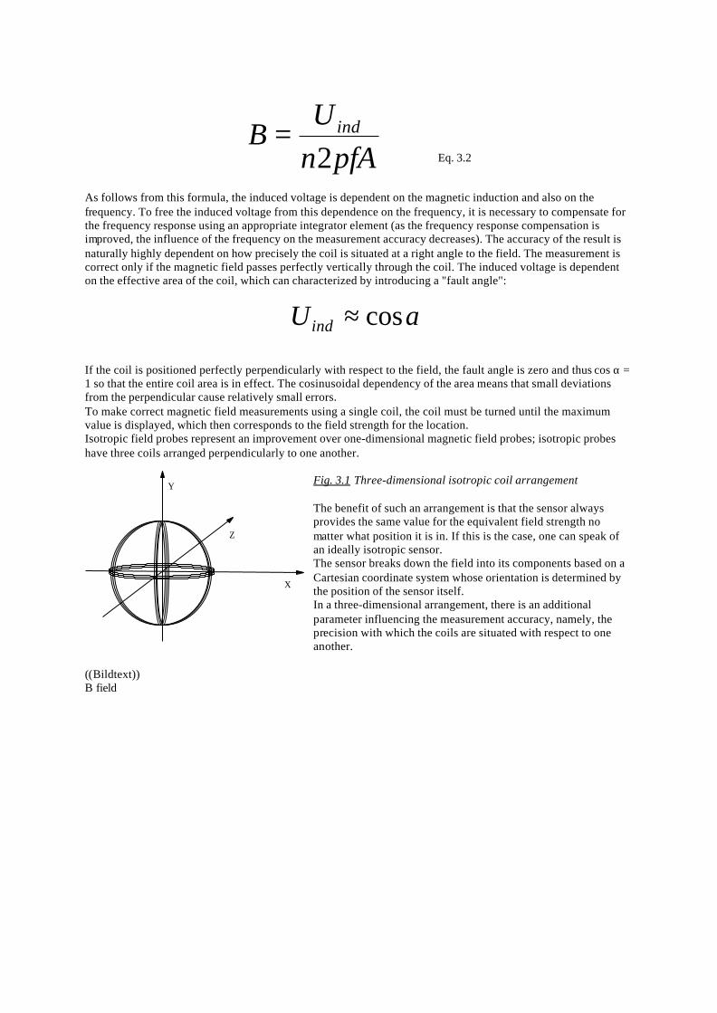
As follows from this formula, the induced voltage is dependent on the magnetic induction and also on thefrequency. To free the induced voltage from this dependence on the frequency, it is necessary to compensate forthe frequency response using an appropriate integrator element (as the frequency response compensation isimproved, the influence of the frequency on the measurement accuracy decreases). The accuracy of the result isnaturally highly dependent on how precisely the coil is situated at a right angle to the field. The measurement iscorrect only if the magnetic field passes perfectly vertically through the coil. The induced voltage is dependenton the effective area of the coil, which can characterized by introducing a "fault angle":

U ind ≈ cosα

If the coil is positioned perfectly perpendicularly with respect to the field, the fault angle is zero and thus cos α =1 so that the entire coil area is in effect. The cosinusoidal dependency of the area means that small deviationsfrom the perpendicular cause relatively small errors.To make correct magnetic field measurements using a single coil, the coil must be turned until the maximumvalue is displayed, which then corresponds to the field strength for the location.Isotropic field probes represent an improvement over one-dimensional magnetic field probes; isotropic probeshave three coils arranged perpendicularly to one another.

Fig. 3.1 Three-dimensional isotropic coil arrangement

The benefit of such an arrangement is that the sensor alwaysprovides the same value for the equivalent field strength nomatter what position it is in. If this is the case, one can speak ofan ideally isotropic sensor.The sensor breaks down the field into its components based on aCartesian coordinate system whose orientation is determined bythe position of the sensor itself.In a three-dimensional arrangement, there is an additionalparameter influencing the measurement accuracy, namely, theprecision with which the coils are situated with respect to oneanother.

((Bildtext))B field

Y

Z

X

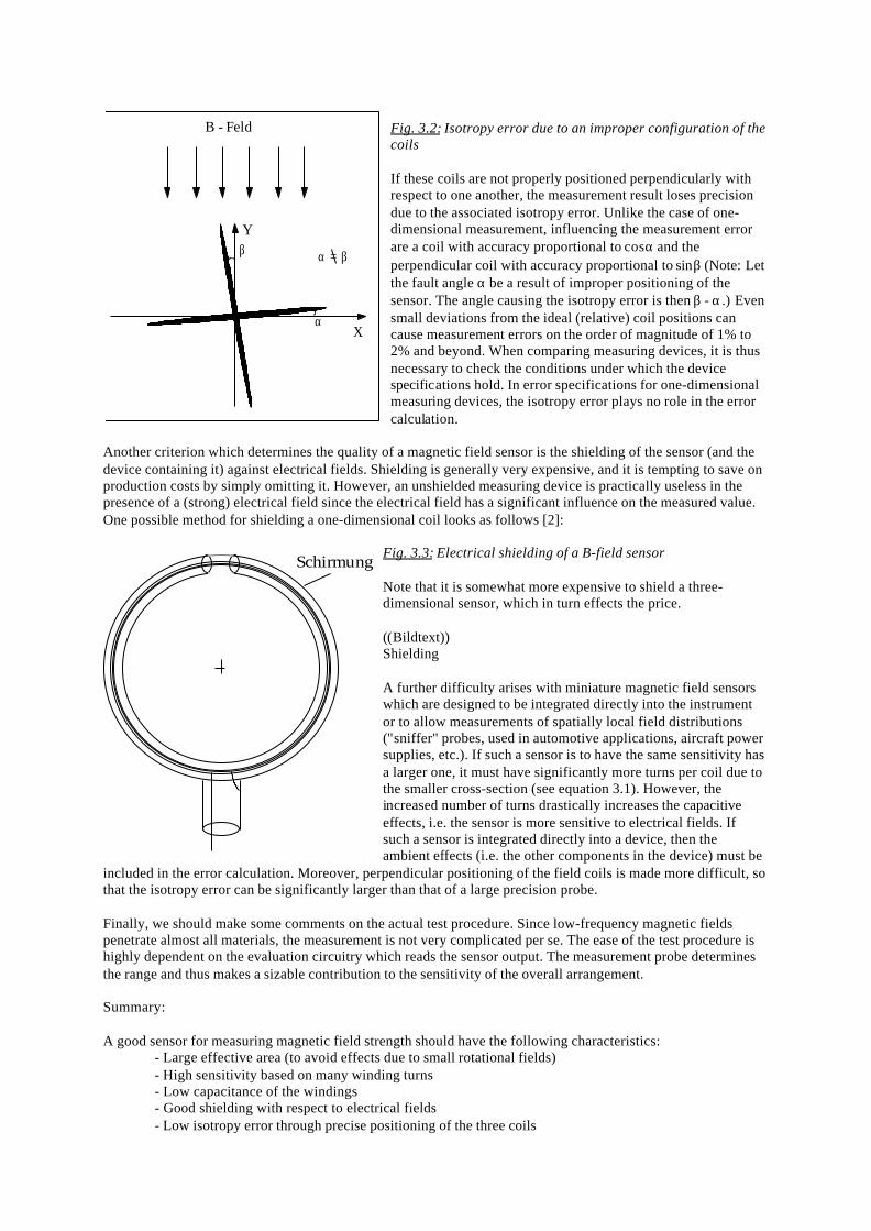
Fig. 3.2: Isotropy error due to an improper configuration of thecoils

If these coils are not properly positioned perpendicularly withrespect to one another, the measurement result loses precisiondue to the associated isotropy error. Unlike the case of one-dimensional measurement, influencing the measurement errorare a coil with accuracy proportional to cosα and theperpendicular coil with accuracy proportional to sinβ (Note: Letthe fault angle α be a result of improper positioning of thesensor. The angle causing the isotropy error is then β - α.) Evensmall deviations from the ideal (relative) coil positions cancause measurement errors on the order of magnitude of 1% to2% and beyond. When comparing measuring devices, it is thusnecessary to check the conditions under which the devicespecifications hold. In error specifications for one-dimensionalmeasuring devices, the isotropy error plays no role in the errorcalculation.

Another criterion which determines the quality of a magnetic field sensor is the shielding of the sensor (and thedevice containing it) against electrical fields. Shielding is generally very expensive, and it is tempting to save onproduction costs by simply omitting it. However, an unshielded measuring device is practically useless in thepresence of a (strong) electrical field since the electrical field has a significant influence on the measured value.One possible method for shielding a one-dimensional coil looks as follows [2]:

Fig. 3.3: Electrical shielding of a B-field sensor

Note that it is somewhat more expensive to shield a three-dimensional sensor, which in turn effects the price.

((Bildtext))Shielding

A further difficulty arises with miniature magnetic field sensorswhich are designed to be integrated directly into the instrumentor to allow measurements of spatially local field distributions("sniffer" probes, used in automotive applications, aircraft powersupplies, etc.). If such a sensor is to have the same sensitivity hasa larger one, it must have significantly more turns per coil due tothe smaller cross-section (see equation 3.1). However, theincreased number of turns drastically increases the capacitiveeffects, i.e. the sensor is more sensitive to electrical fields. Ifsuch a sensor is integrated directly into a device, then theambient effects (i.e. the other components in the device) must be

included in the error calculation. Moreover, perpendicular positioning of the field coils is made more difficult, sothat the isotropy error can be significantly larger than that of a large precision probe.

Finally, we should make some comments on the actual test procedure. Since low-frequency magnetic fieldspenetrate almost all materials, the measurement is not very complicated per se. The ease of the test procedure ishighly dependent on the evaluation circuitry which reads the sensor output. The measurement probe determinesthe range and thus makes a sizable contribution to the sensitivity of the overall arrangement.

Summary:

A good sensor for measuring magnetic field strength should have the following characteristics:- Large effective area (to avoid effects due to small rotational fields)- High sensitivity based on many winding turns- Low capacitance of the windings- Good shielding with respect to electrical fields- Low isotropy error through precise positioning of the three coils

α

βY

X

B - Feld

α = β

Schirmung

- Standard dimensions- Good mechanical stability- Flexibility

Of course the sensor cannot be considered in isolation since the input amplifiers which process the inducedvoltage of the sensor also play a role. In other words, the sensitivity of the test setup can be altered by thenumber of winding turns used in the sensor and also by the sensitivity of the input circuits.

The design used for the magnetic field sensors in products from Wandel & Goltermann looks as follows:To allow the order of magnitude of a magnetic field to be determined even without an external sensor, a small,three-dimensional isotropic sensor is integrated directly into the basic device. When no external precision probeis connected, the measurement is automatically executed using this internal B-field probe.The internal sensor coils are positioned relative to one another such that the device itself has the smallestpossible effect on the isotropy. Since, for example, the presence of batteries can "bend" the magnetic field, it isnot possible to totally eliminate such effects, but they are at least minimized. The additional shielding measuresto counter electrical fields allow this arrangement to achieve a measurement accuracy of approx. 5%, which ratesas very good. The internal sensor is individually calibrated in production for each device.

For applications requiring standardized (and precise) measurement of magnetic fields, a precision probeconforming to VDE 0848 with an effective cross-section of 100 cm2 is available. The best possiblemeasurement accuracy is attained with this probe. The isotropy error of this three-dimensional probe ranges fromonly approx. 0.5% to 1%. The probe has good shielding against electrical fields as well as a very ruggedmechanical design. An electrical field of 100 kV/m results in a measurement error of approx. 50 nT to 100 nT.The good reproducibility in production allows us to store a single calibration data set in the device which isrepresentative of all precision probes. Measurement accuracies of 2% to 3% are possible with this probe.

For measuring magnetic fields in hard to access spaces or for recording local fields in a small area, theaccessories include a miniature, three-dimensional, isotropic probe. To achieve the greatest degree of precisionpossible with such probes (given their problematic nature), they are especially calibrated and the calibration dataare stored directly in the probe.These details, combined with suitable shielding against electrical fields, yield measured values with an accuracyof approx. 4% to 5%.

The specifications for the accuracy of the probes always refer to a frequency and field strength range. Uponspecial request, these devices can also be calibrated at user-specified frequencies for improved accuracy at thefrequencies of interest.

3.2 Technique for measuring electrical fields

The most common method for measuring electrical fields is the capacitive method. Two electrodes (dipole,antenna) are brought into the electrical field to be measured and the displacement current is measured. Thenature of the electrodes varies depending on the application. Since we are considering only low-frequencyelectrical fields here, the size of the sensor is of no practical consequence (basically, however, smaller sensorsare better suited to measurements at higher frequencies).Compared to magnetic fields, measurement of electrical fields is somewhat more complicated. Since bodiespresent in the electrical field distort the field, special precautions must be taken to ensure reliable results.

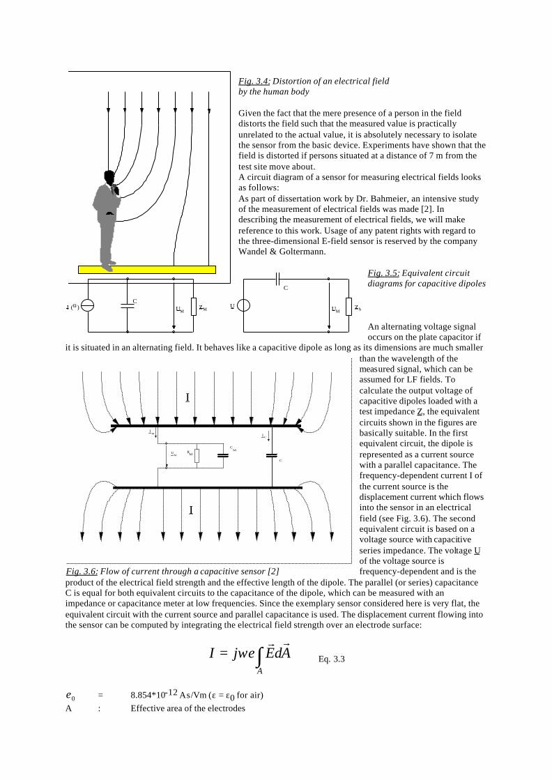
Fig. 3.4: Distortion of an electrical fieldby the human body

Given the fact that the mere presence of a person in the fielddistorts the field such that the measured value is practicallyunrelated to the actual value, it is absolutely necessary to isolatethe sensor from the basic device. Experiments have shown that thefield is distorted if persons situated at a distance of 7 m from thetest site move about.A circuit diagram of a sensor for measuring electrical fields looksas follows:As part of dissertation work by Dr. Bahmeier, an intensive studyof the measurement of electrical fields was made [2]. Indescribing the measurement of electrical fields, we will makereference to this work. Usage of any patent rights with regard tothe three-dimensional E-field sensor is reserved by the companyWandel & Goltermann.

Fig. 3.5: Equivalent circuitdiagrams for capacitive dipoles

An alternating voltage signaloccurs on the plate capacitor if

it is situated in an alternating field. It behaves like a capacitive dipole as long as its dimensions are much smallerthan the wavelength of themeasured signal, which can beassumed for LF fields. Tocalculate the output voltage ofcapacitive dipoles loaded with atest impedance Z, the equivalentcircuits shown in the figures arebasically suitable. In the firstequivalent circuit, the dipole isrepresented as a current sourcewith a parallel capacitance. Thefrequency-dependent current I ofthe current source is thedisplacement current which flowsinto the sensor in an electricalfield (see Fig. 3.6). The secondequivalent circuit is based on avoltage source with capacitiveseries impedance. The voltage Uof the voltage source isfrequency-dependent and is the

product of the electrical field strength and the effective length of the dipole. The parallel (or series) capacitanceC is equal for both equivalent circuits to the capacitance of the dipole, which can be measured with animpedance or capacitance meter at low frequencies. Since the exemplary sensor considered here is very flat, theequivalent circuit with the current source and parallel capacitance is used. The displacement current flowing intothe sensor can be computed by integrating the electrical field strength over an electrode surface:

∫=A

AdEjIrr

ωε Eq. 3.3

ε0 = 8.854*10-12 As/Vm (ε = ε0 for air)A : Effective area of the electrodes

UMZM UM

ZMI (ω )C

C

U

C

UM

MC

MR

IM I C

I

I

Fig. 3.6: Flow of current through a capacitive sensor [2]

The current I produces a voltage on the electrodes or on the input impedance of the measurement circuitryconnected in parallel to the electrodes. The input impedance of the measurement circuitry is determined by ahigh-impedance source follower in order to achieve the greatest possible frequency range with no dependence onfrequency. This input capacitance CM of the source follower is in parallel to the plate capacitance. The voltageUM which occurs on the sensor plates and thus at the input to the measurement circuitry is given by:

)(1CCj

R

AdEj

ZIZIUM

M

AgesMMM

++===

∫

ω

ωεrr

Eq. 3.4

With the assumed test impedance ZM the sensor represents a 1st order high-pass filter (see the equivalent circuit

diagram). Its limit frequency is

fR C Cg

M M

=+

12π ( ) eq. 3.5

At frequencies well above the limit frequency, the input admittance of the measurement circuitry can beneglected with respect to the susceptance of the capacitive elements:

1/RM << ω(C+CM)

Equation 3.4 is thus simplified as follows:

M

AM CC

AdEU

+=

∫rr

ε

Eq. 3.6

According to this equation, measurement of the electrical field strength is independent of frequency above thelower limit frequency. To extend the lower limit frequency downwards and produce a sensor that is as broadbandas possible, the ohmic resistance of the measurement circuitry must be maximized.Since we are limiting our scope to low-frequency fields, the theoretical considerations with regard to an upperlimit frequency at approx. 180 MHz do not come into play.

Based on these theoretical considerations, we will show how the mechanism of a capacitive sensor is used tomeasure the electrical field. In the relevant literature and in (current) publications, it is this test setup which isfound, if anything.Theoretical considerations will not be further examined here since the named references cover them in depth.

In the following section, we will consider the practical implementation of this measurement technique in a sensorwhich rounds out the array of sensors available in our line of field measurement products. As far as we can tell,this sensor is the only one of its type on the market. It has the ability to measure electrical fields three-dimensionally and selectively, i.e. it is fully isotropic. The measurement accuracy which is achieved is superiorby far to that of many commercially available one-dimensional sensors. Most noteworthy is its cubical shape.

((Bildtext))Fiber optical cableSensor surfaces

Fig. 3.7: Three-dimensional isotropic sensor for measuringelectrical field strength

This technique was examined by Dr. Bahmeier in both its theoreticaland practical aspects as part of his dissertation work. In cooperationwith Dr. Bahmeier, we carried on with the development of thistechnique, making it suitable for series production. Interested readersshould consult his dissertation for details of the theoretical aspectsand the related practical measurement results [2].The technique described for capacitive measurement is used here forthree-dimensional measurement. The sensor has three platesarranged perpendicularly to one another, each of which forms acapacitance with respect to the core of the cube. For reasons of

symmetry, another plate was arranged opposite each of these three "active" plates, but the "inactive" plates donot enter into the measurement. The three field components are determined by measuring the displacementcurrents of the individual plates. These signals are sampled via three input amplifiers and multiplexer stages andprocessed by a signal processor. This makes it possible to break down the field components by spectrum andmeasure the fields selectively. All of the digital signal processing electronics is situated within the actual sensor.Only the computed components are transmitted to the basic device. This minimizes the data stream and therebyincreases the lifespan of the rechargeable cell installed in the sensor. To minimize distortion of the electricalfield, the data from the sensor are transmitted via fiber optical cables (max. length 20 m). The sensor is thus fullyremote-controllable from the basic device.One very interesting question concerns the isotropy of this structure. An isotropic sensor provides the same valuefor the equivalent field strength in every position with respect to the field. The theoretical verification beingquite complicated, interested readers should consult the above work. A practical proof of the isotropic behaviorof the sensor is illustrated hereafter:

((Bildtext))SensorStyrofoamFiber optics ((LWL))Rotary tableAngle indicatorInterface

Fig. 3.8: Test setup for measuringisotropy [2]

((Bildtext))Angle of rotation

The test setup consists of twoopposite plates which are used togenerate a defined electrical field.A rotary table is situated in theactual field, the table beingremote-controlled via a computer.The sensor is first laid on one sideand rotated. The evaluationcircuitry is located outside of thefield and is connected to thesensor via a fiber optical cable.This evaluation circuitry providesthe current measured data to thecomputer, which then computes

the equivalent field strength based on thesedata. The following figure shows the resultsof this computation:

Fig. 3.9: Results of the isotropy measurementwith the sensor on its side [2]

Lichtwellenleiter

Sensorflächen

Sensor

LWLStyropor

DrehtellerInterface

Winkelgeber

0 30 60 90-30-60-900

5

10

15

20

25

30

35

40

E [V/m]

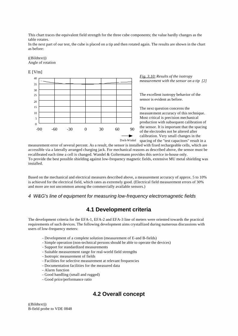
This chart traces the equivalent field strength for the three cube components; the value hardly changes as thetable rotates.In the next part of our test, the cube is placed on a tip and then rotated again. The results are shown in the chartas before:

((Bildtext))Angle of rotation

Fig. 3.10: Results of the isotropymeasurement with the sensor on a tip [2]

The excellent isotropy behavior of thesensor is evident as before.

The next question concerns themeasurement accuracy of this technique.Most critical is precision mechanicalproduction with subsequent calibration ofthe sensor. It is important that the spacingof the electrodes not be altered aftercalibration. Very small changes in thespacing of the "test capacitors" result in a

measurement error of several percent. As a result, the sensor is installed with fixed rechargeable cells, which areaccessible via a laterally arranged charging jack. For mechanical reasons as described above, the sensor must berecalibrated each time a cell is changed. Wandel & Goltermann provides this service in-house only.To provide the best possible shielding against low-frequency magnetic fields, extensive MU metal shielding wasinstalled.

Based on the mechanical and electrical measures described above, a measurement accuracy of approx. 5 to 10%is achieved for the electrical field, which rates as extremely good. (Electrical field measurement errors of 30%and more are not uncommon among the commercially available sensors.)

4 W&G's line of equipment for measuring low-frequency electromagnetic fields

4.1 Development criteria

The development criteria for the EFA-1, EFA-2 and EFA-3 line of meters were oriented towards the practicalrequirements of such devices. The following development aims crystallized during numerous discussions withusers of low-frequency meters:

- Development of a complete solution (measurement of E-and B-fields)- Simple operation (non-technical persons should be able to operate the devices)- Support for standardized measurements- Suitable measurement range for real-world field strengths- Isotropic measurement of fields- Facilities for selective measurement at relevant frequencies- Documentation facilities for the measured data- Alarm function- Good handling (small and rugged)- Good price/performance ratio

4.2 Overall concept

((Bildtext))B-field probe to VDE 0848

0 30 60 90-30-60-900

5

10

15

20

25

30

35

40

E [V/m]

Dreh-Winkel

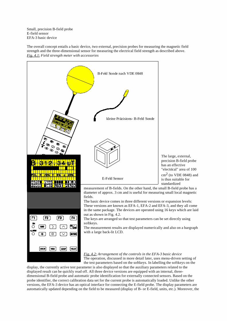
Small, precision B-field probeE-field sensorEFA-3 basic device

The overall concept entails a basic device, two external, precision probes for measuring the magnetic fieldstrength and the three-dimensional sensor for measuring the electrical field strength as described above.Fig. 4.1: Field strength meter with accessories

The large, external,precision B-field probehas an effective"electrical" area of 100

cm2 (to VDE 0848) andis thus suitable forstandardized

measurement of B-fields. On the other hand, the small B-field probe has adiameter of approx. 3 cm and is useful for measuring small local magneticfields.The basic device comes in three different versions or expansion levels:These versions are known as EFA-1, EFA-2 and EFA-3, and they all comein the same package. The devices are operated using 16 keys which are laidout as shown in Fig. 4.2.The keys are arranged so that test parameters can be set directly usingsoftkeys.The measurement results are displayed numerically and also on a bargraphwith a large back-lit LCD.

Fig. 4.2: Arrangement of the controls in the EFA-3 basic deviceThe operation, discussed in more detail later, uses menu-driven setting ofthe test parameters based on the softkeys. In labelling the softkeys on the

display, the currently active test parameter is also displayed so that the auxiliary parameters related to thedisplayed result can be quickly read off. All three device versions are equipped with an internal, three-dimensional B-field probe and automatic probe identification for externally connected sensors. Based on theprobe identifier, the correct calibration data set for the current probe is automatically loaded. Unlike the otherversions, the EFA-3 device has an optical interface for connecting the E-field probe. The display parameters areautomatically updated depending on the field to be measured (display of B- or E-field, units, etc.). Moreover, the

Basisgerät EFA-3 E-Feld Sensor

B-Feld Sonde nach VDE 0848

kleine Präzisions- B-Feld Sonde

test data can be transferred directly to a printer or computer via an optical RS-232 interface. The devices can beoperated from batteries or rechargeable cells; the latter are recharged via a charging jack on the device.

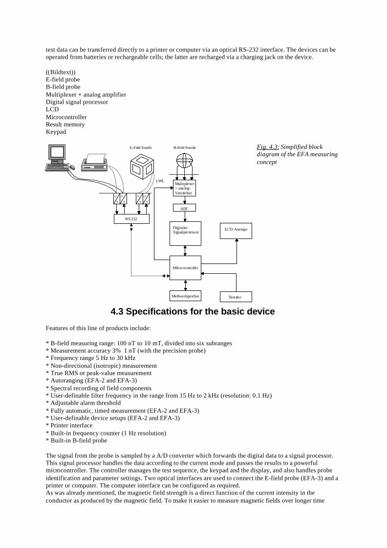
((Bildtext))E-field probeB-field probeMultiplexer + analog amplifierDigital signal processorLCDMicrocontrollerResult memoryKeypad

Fig. 4.3: Simplified blockdiagram of the EFA measuringconcept

4.3 Specifications for the basic device

Features of this line of products include:

* B-field measuring range: 100 nT to 10 mT, divided into six subranges* Measurement accuracy 3% 1 nT (with the precision probe)* Frequency range 5 Hz to 30 kHz* Non-directional (isotropic) measurement* True RMS or peak-value measurement* Autoranging (EFA-2 and EFA-3)* Spectral recording of field components* User-definable filter frequency in the range from 15 Hz to 2 kHz (resolution: 0.1 Hz)* Adjustable alarm threshold* Fully automatic, timed measurement (EFA-2 and EFA-3)* User-definable device setups (EFA-2 and EFA-3)* Printer interface* Built-in frequency counter (1 Hz resolution)* Built-in B-field probe

The signal from the probe is sampled by a A/D converter which forwards the digital data to a signal processor.This signal processor handles the data according to the current mode and passes the results to a powerfulmicrocontroller. The controller manages the test sequence, the keypad and the display, and also handles probeidentification and parameter settings. Two optical interfaces are used to connect the E-field probe (EFA-3) and aprinter or computer. The computer interface can be configured as required.As was already mentioned, the magnetic field strength is a direct function of the current intensity in theconductor as produced by the magnetic field. To make it easier to measure magnetic fields over longer time

Multiplexer+ ana log-Verstärker

ADC

DigitalerSignalprozessor

Mikrocontroller

LCD-Anzeige

TastaturMeßwertspeicher

E-Feld Sonde B-Feld Sonde

O

E

O

E

O

E

O

E

RS 232

LWL

frames, the EFA-2 and EFA-3 device versions include fully automatic, timed measurement capabilities. Thiscapability also exists in the EFA-3 for measuring electrical fields. The measured data recorded over a maximuminterval of 24 h can be easily transferred to a computer for further processing.

4.4 Operation and applications of the devices

Operation of these devices is made simple by their menu-driven controls and clear display of test parameters.The following four main menus can be directly accessed from any device setting using four distinct keys:

TEST menu: For displaying measurement results and setting test parametersCONFIGURATION menu: For setting device parametersMEMORY menu: For programming automatic (timed) measurementsUSER menu: For storing and recalling device setups

Taking the TEST menu as an example (this menu appears when the device is powered up), we'll take a closerlook at the basic operation of these devices:

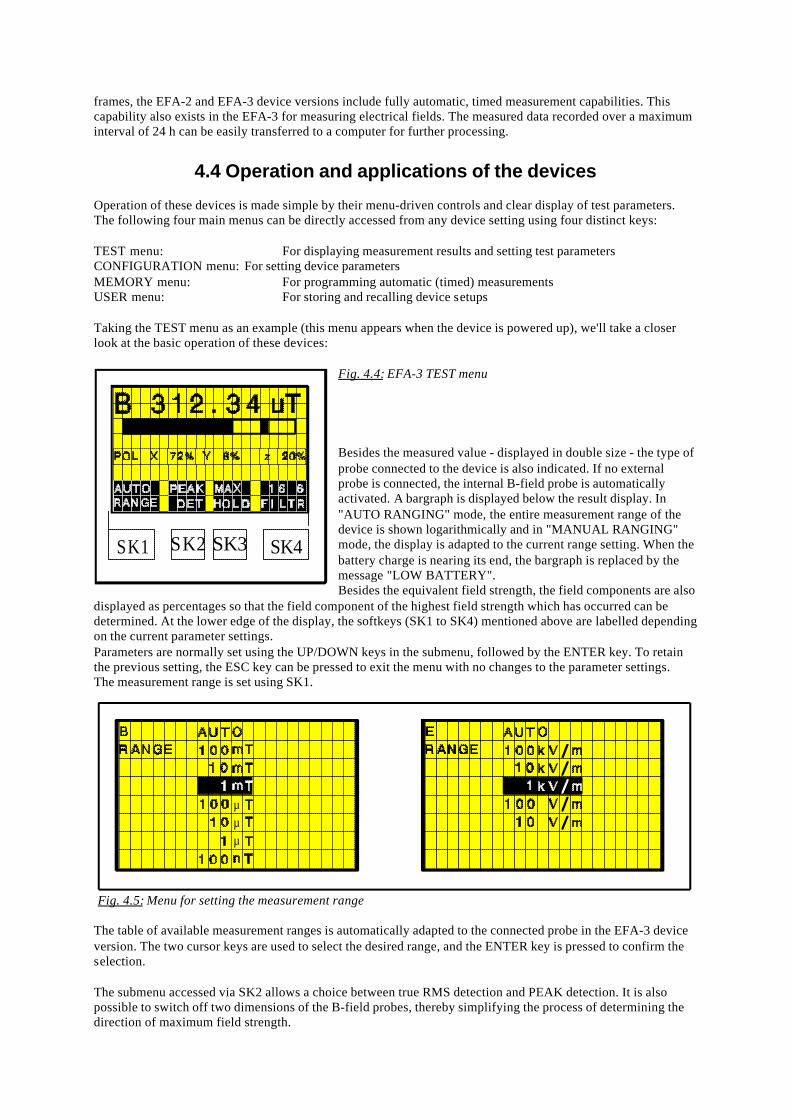
Fig. 4.4: EFA-3 TEST menu

Besides the measured value - displayed in double size - the type ofprobe connected to the device is also indicated. If no externalprobe is connected, the internal B-field probe is automaticallyactivated. A bargraph is displayed below the result display. In"AUTO RANGING" mode, the entire measurement range of thedevice is shown logarithmically and in "MANUAL RANGING"mode, the display is adapted to the current range setting. When thebattery charge is nearing its end, the bargraph is replaced by themessage "LOW BATTERY".Besides the equivalent field strength, the field components are also

displayed as percentages so that the field component of the highest field strength which has occurred can bedetermined. At the lower edge of the display, the softkeys (SK1 to SK4) mentioned above are labelled dependingon the current parameter settings.Parameters are normally set using the UP/DOWN keys in the submenu, followed by the ENTER key. To retainthe previous setting, the ESC key can be pressed to exit the menu with no changes to the parameter settings.The measurement range is set using SK1.

The table of available measurement ranges is automatically adapted to the connected probe in the EFA-3 deviceversion. The two cursor keys are used to select the desired range, and the ENTER key is pressed to confirm theselection.

The submenu accessed via SK2 allows a choice between true RMS detection and PEAK detection. It is alsopossible to switch off two dimensions of the B-field probes, thereby simplifying the process of determining thedirection of maximum field strength.

SK2 SK3SK1 SK4

µµµ

Fig. 4.5: Menu for setting the measurement range

To make it easy to determine the maximum field strength which has occurred, the display can be switched toMAX HOLD; the data are still updated in the bargraph. The displayed value is then equal to the maximum fieldstrength measured since the display was switched to this mode.

One innovative feature of these devices is the ability to make both selective and broadband field measurements.The following band limits (and filter frequencies) are available:

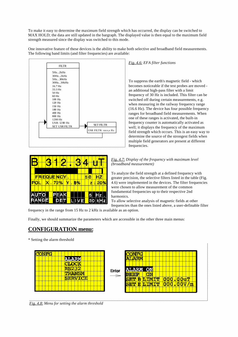
Fig. 4.6: EFA filter functions

To suppress the earth's magnetic field - whichbecomes noticeable if the test probes are moved -an additional high-pass filter with a limitfrequency of 30 Hz is included. This filter can beswitched off during certain measurements, e.g.when measuring in the railway frequency range(16.6 Hz). The device has four possible frequencyranges for broadband field measurements. Whenone of these ranges is activated, the built-infrequency counter is automatically activated aswell; it displays the frequency of the maximumfield strength which occurs. This is an easy way todetermine the source of the strongest fields whenmultiple field generators are present at differentfrequencies.

Fig. 4.7: Display of the frequency with maximum level(broadband measurement)

To analyze the field strength at a defined frequency withgreater precision, the selective filters listed in the table (Fig.4.6) were implemented in the devices. The filter frequencieswere chosen to allow measurement of the commonfundamental frequencies up to their respective 2ndharmonics.To allow selective analysis of magnetic fields at otherfrequencies than the ones listed above, a user-definable filter

frequency in the range from 15 Hz to 2 kHz is available as an option.

Finally, we should summarize the parameters which are accessible in the other three main menus:

CONFIGURATION menu:

* Setting the alarm threshold

FILTR

5Hz...2kHz30Hz...2kHz5Hz...30kHz30Hz...30kHz16.7 Hz33.3 Hz50 Hz60 Hz100 Hz120 Hz150 Hz180 Hz400 Hz800 Hz1200 HzUSR: 1280 HzSET USR FILTR SET FILTR

USR FILTR: xxxx,x Hz

Fig. 4.8: Menu for setting the alarm threshold

The alarm threshold can be set anywhere in the entire measurement range. The alarm is triggered when thisthreshold is exceeded. Besides a visible alarm, an audible signal can also be output (function can be disabled).

Note: In the EFA-3 device version, the appropriate alarm threshold is activated if the alarm is switched ondepending on the probe which is connected.

* Setting the built-in clock (CLOCK)* Configuration of the optical RS-232 interface (RS232)* Configuration of the (result) data transfer rate (to the printer) (TRANS)* Switching between the units TESLA - GAUSS (SERVICE)

MEMORY menu:

Timed measurements are programmed in the MEMORY menu. Up to 2000 sets of results can be stored; thesettings associated with the measured value can be reproduced from a given set of results:

* Entry of time of day "Start measurement"* Entry of time of day "Stop measurement"* Entry of step-size for two successive measurements* Show function for displaying stored values* Print function for outputting the memory content* Clear function for erasing the entire memory content or individual locations

USER menu:

* Recalling the default device setup* Function for storing device setups* Function for recalling a previously stored setup

Up to four user-definable device setups can be stored.

4.5 Device calibration

Calibration is an important prerequisite for reproducible measurements and standardized verification of fieldstrengths. In the devices in the EFA series, a compensation data set is stored for each sensor used; the data forthe current sensor are used in computing results. The data set contains information on the frequency responseand level compensation required for the particular probe. The measured data for the probes are selectivelyrecorded and stored for the three dimensions. The production process includes measurement of the isotropy ofthe built-in probe, thereby making it possible to guarantee the device specifications.To eliminate the need to pair up the device with a particular external probe, the compensation data set is storeddirectly in each (external) probe.The magnetic field probes are calibrated in a "standard magnetic field" which is generated using a Helmholtzframe. Based on a comparison standard calibrated by the Federal German Bureau of Standards (PTB), therequired field generation precision can be continually checked and verified.The sensor for measuring the electrical field is calibrated in a similar manner to the B-field sensor, i.e. using a"standardized field" based on a plate construction which is likewise traceable to a "field standard" of the PTB.

5 The EFA-1, EFA-2 and EFA-3 device versions

All device versions have the same measurement accuracy and employ the same probes for measuring low-frequency magnetic fields. The EFA-2 and EFA-2 basic devices are identical up to the capability to connect thesensor for measuring electrical field strength (EFA-3), and have the same features described above.In the low-cost version (EFA-1), the following features are missing: autoranging, timed measurement andstorage of device setups.

6 Bibliography

[1] Elektrische und magnetische Felder[English translation of title: Electrical and Magnetic Fields]Strom im AlltagIZE Informationszentrale der Elektrizitätswirtschaft E.V.Frankfurt (Germany)

[2] Dissertation, Dipl. Ing. Georg BahmeierVDI VerlagSeries 8, No. 438ISBN 3-18-343808-9