12 Intertemporal Choice - School of Arts & Sciencesvr0j/econ10205/lectures/fluct...Copyright © 2005 Pearson Addison-Wesley. All rights reserved. 8-6 Figure 8.4 A Consumer Who Is a

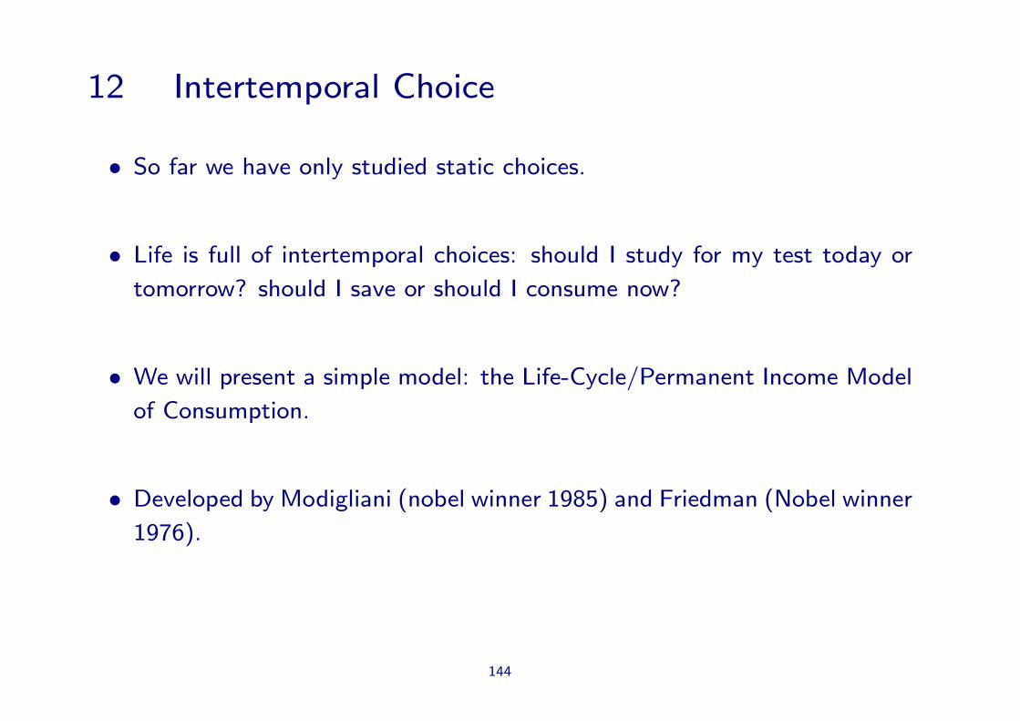
12 Intertemporal Choice

• So far we have only studied static choices.

• Life is full of intertemporal choices: should I study for my test today or

tomorrow? should I save or should I consume now?

• We will present a simple model: the Life-Cycle/Permanent Income Model

of Consumption.

• Developed by Modigliani (nobel winner 1985) and Friedman (Nobel winner

1976).

144

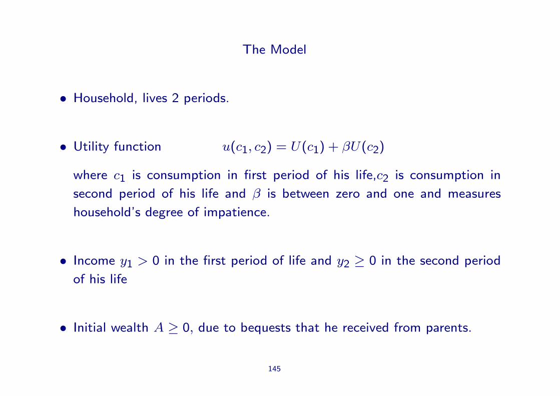
The Model

• Household, lives 2 periods.

• Utility function u(c1, c2) = U(c1) + βU(c2)

where c1 is consumption in first period of his life,c2 is consumption in

second period of his life and β is between zero and one and measures

household’s degree of impatience.

• Income y1 > 0 in the first period of life and y2 ≥ 0 in the second period

of his life

• Initial wealth A ≥ 0, due to bequests that he received from parents.

145

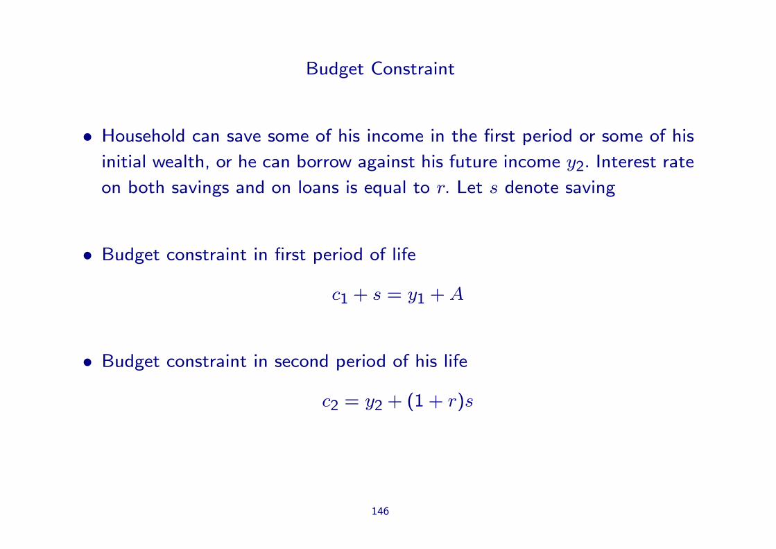
Budget Constraint

• Household can save some of his income in the first period or some of his

initial wealth, or he can borrow against his future income y2. Interest rate

on both savings and on loans is equal to r. Let s denote saving

• Budget constraint in first period of life

c1 + s = y1 + A

• Budget constraint in second period of his life

c2 = y2 + (1 + r)s

146

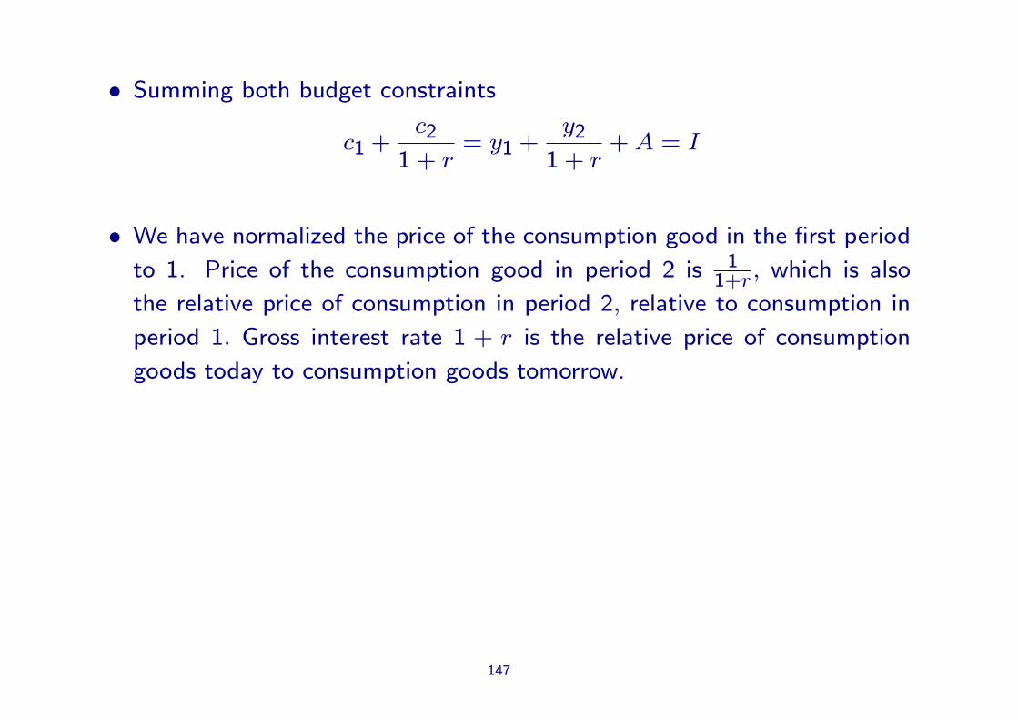
• Summing both budget constraints

c1 +c2

1 + r= y1 +

y2

1 + r+ A = I

• We have normalized the price of the consumption good in the first period

to 1. Price of the consumption good in period 2 is 11+r, which is also

the relative price of consumption in period 2, relative to consumption in

period 1. Gross interest rate 1 + r is the relative price of consumption

goods today to consumption goods tomorrow.

147

Key Results

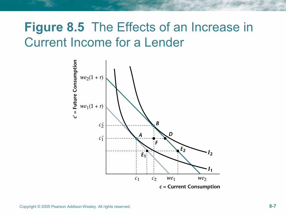
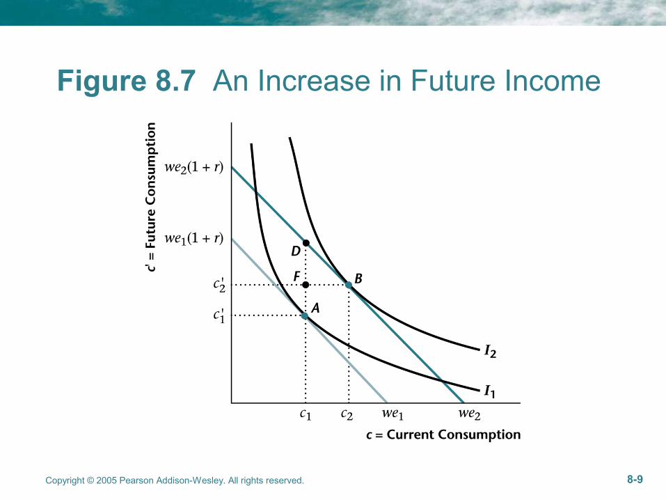
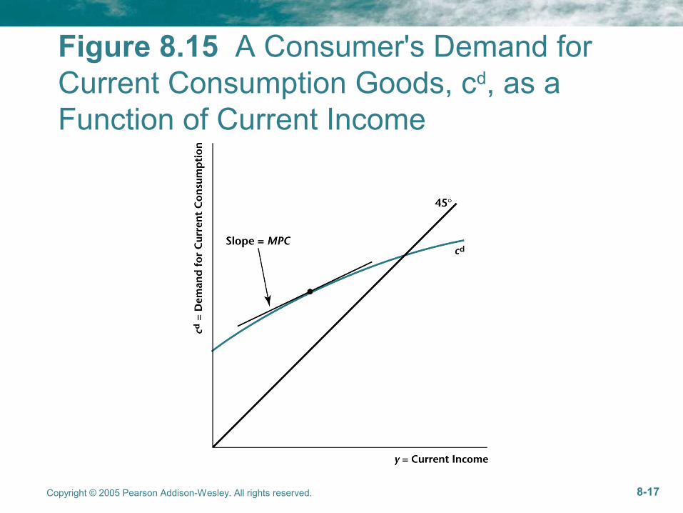
• What variables does current consumption depend on? y1, y2, A, r.

• What happens to consumption if y1, y2 or A increases?

• Both c1 and c2 increase.

148

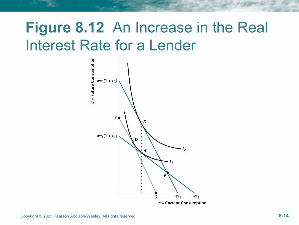
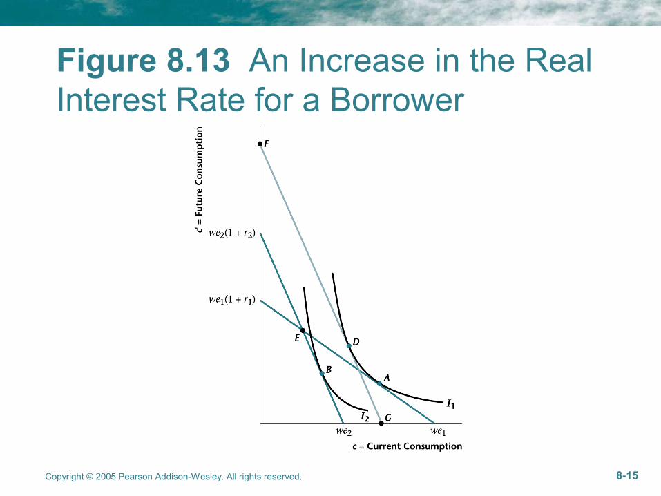
Comparative Statics: Changes in the Interest Rate

• Income effect: if a saver, then higher interest rate increases income for

given amount of saving. Increases consumption in first and second period.

If borrower, then income effect negative for c1 and c2.

• Substitution effect: gross interest rate 1+r is relative price of consumption

in period 1 to consumption in period 2. c1 becomes more expensive relative

to c2. This increases c2 and reduces c1.

• Hence: for a saver an increase in r increases c2 and may increase or

decrease c1. For a borrower an increase in r reduces r1 and may increase

or decrease c2.

149

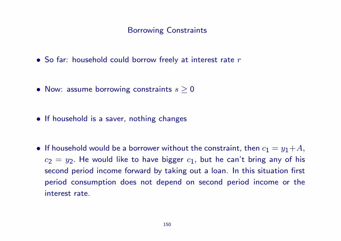
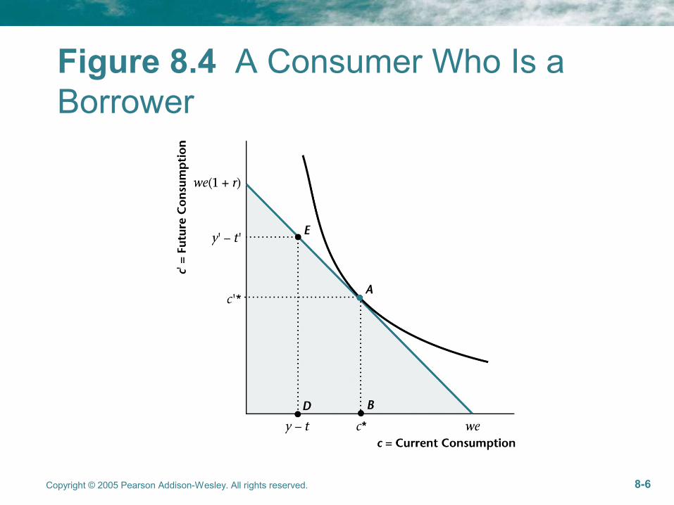
Borrowing Constraints

• So far: household could borrow freely at interest rate r

• Now: assume borrowing constraints s ≥ 0

• If household is a saver, nothing changes

• If household would be a borrower without the constraint, then c1 = y1+A,

c2 = y2. He would like to have bigger c1, but he can’t bring any of his

second period income forward by taking out a loan. In this situation first

period consumption does not depend on second period income or the

interest rate.

150

Chapter 8

A Two-Period Model: The Consumption-Savings Decision and Ricardian Equivalence

Copyright © 2005 Pearson Addison-Wesley. All rights reserved. 8-2

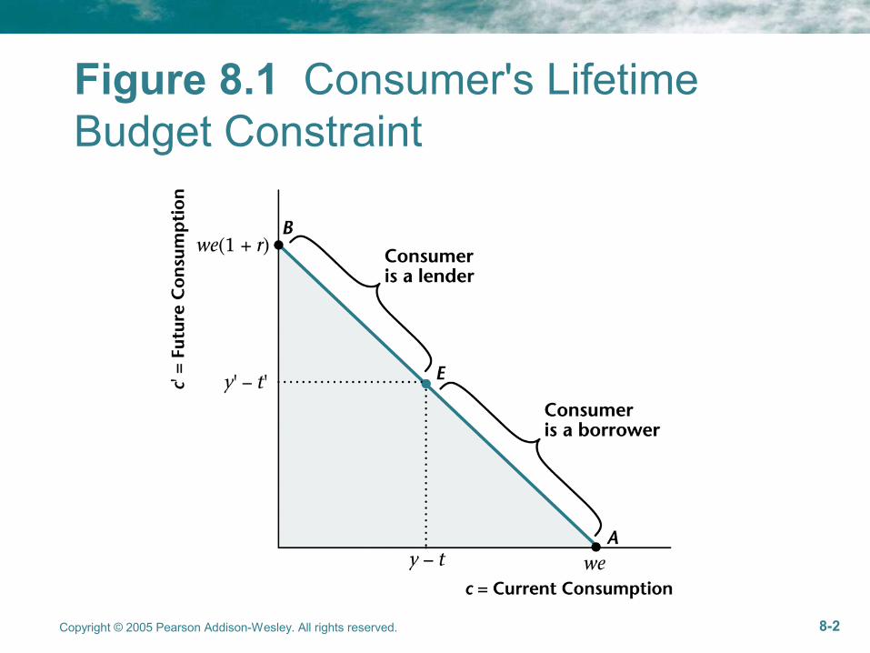
Figure 8.1 Consumer's Lifetime Budget Constraint


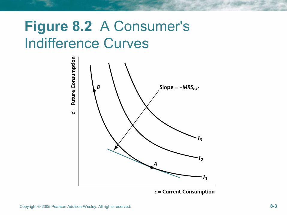
Figure 8.2 A Consumer's Indifference Curves


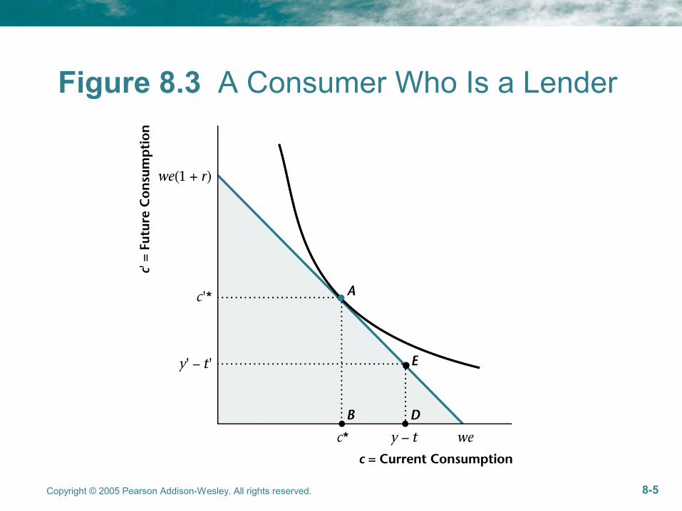
Figure 8.3 A Consumer Who Is a Lender


Figure 8.4 A Consumer Who Is a Borrower


Figure 8.5 The Effects of an Increase in Current Income for a Lender


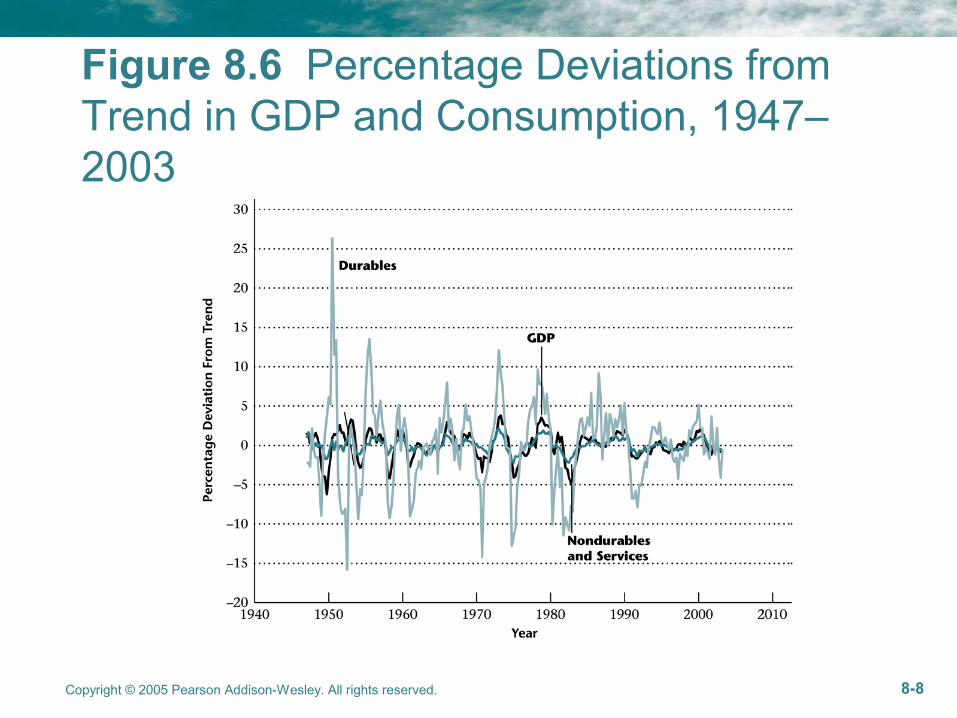
Figure 8.6 Percentage Deviations from Trend in GDP and Consumption, 1947–2003


Figure 8.7 An Increase in Future Income


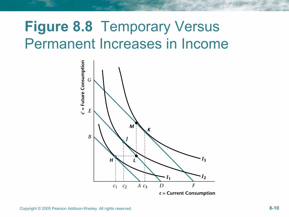
Figure 8.8 Temporary Versus Permanent Increases in Income


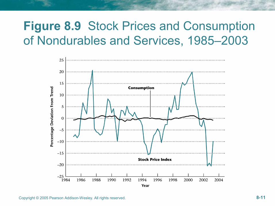
Figure 8.9 Stock Prices and Consumption of Nondurables and Services, 1985–2003


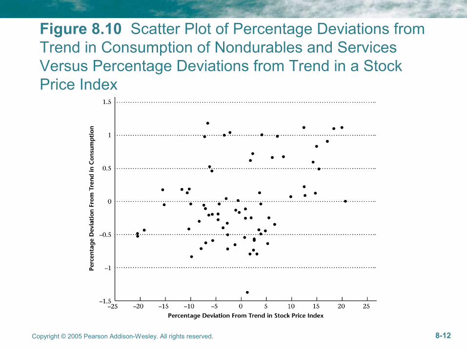
Figure 8.10 Scatter Plot of Percentage Deviations from Trend in Consumption of Nondurables and Services Versus Percentage Deviations from Trend in a Stock Price Index


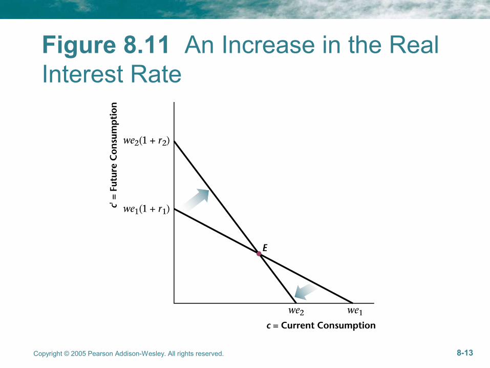
Figure 8.11 An Increase in the Real Interest Rate


Figure 8.12 An Increase in the Real Interest Rate for a Lender


Figure 8.13 An Increase in the Real Interest Rate for a Borrower


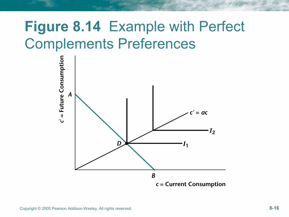
Figure 8.14 Example with Perfect Complements Preferences


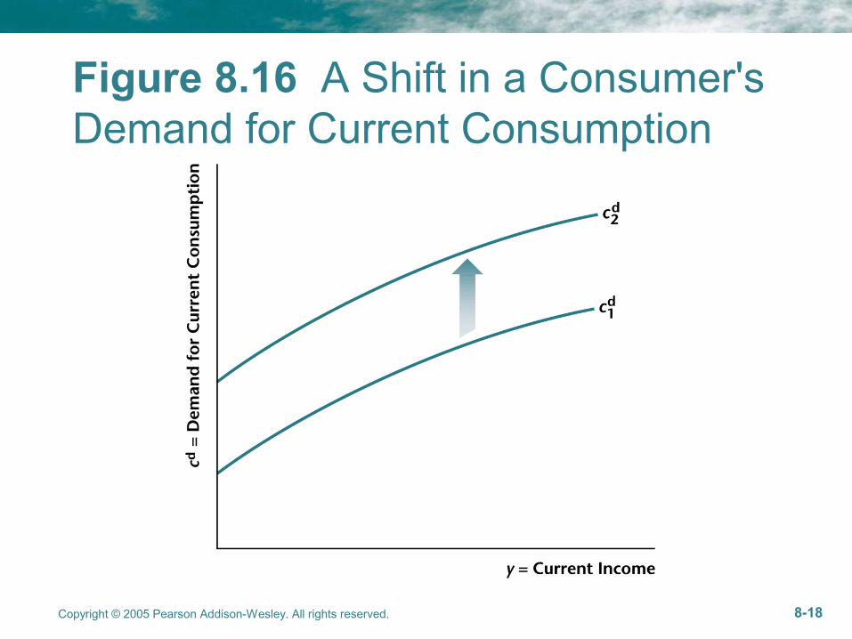
Figure 8.15 A Consumer's Demand for Current Consumption Goods, cd, as a Function of Current Income


Figure 8.16 A Shift in a Consumer's Demand for Current Consumption


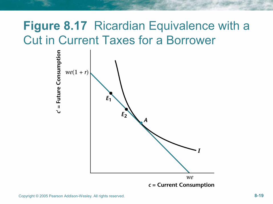
Figure 8.17 Ricardian Equivalence with a Cut in Current Taxes for a Borrower


Figure 8.18 Pay-As-You-Go Social Security for Consumers Who Are Old in Period T


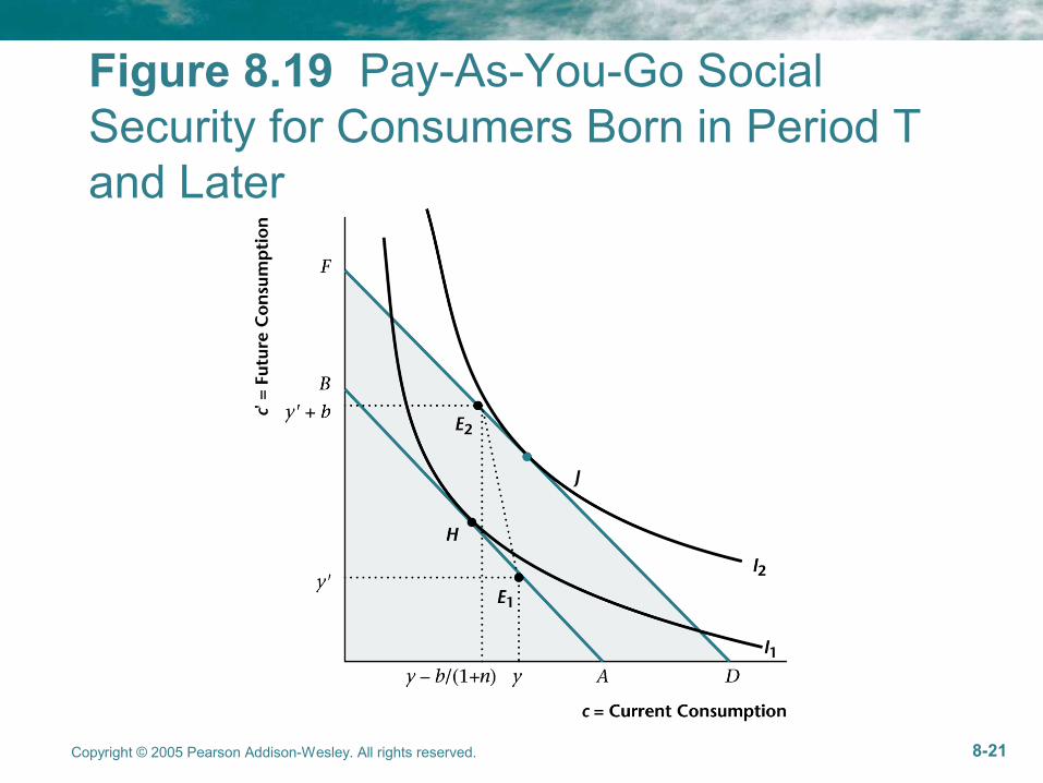
Figure 8.19 Pay-As-You-Go Social Security for Consumers Born in Period T and Later


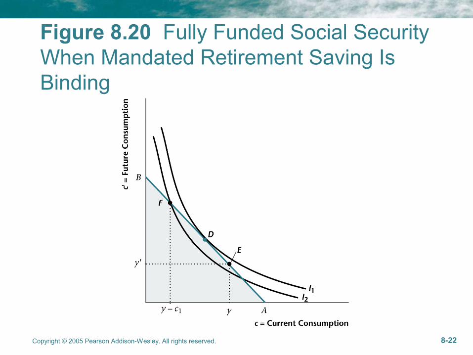
Figure 8.20 Fully Funded Social Security When Mandated Retirement Saving Is Binding


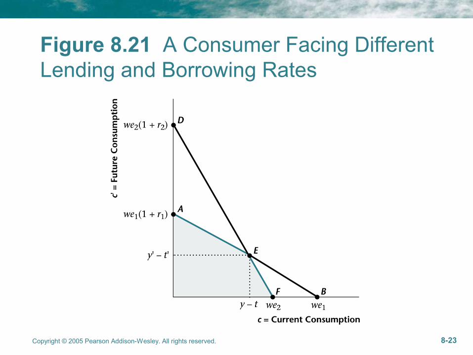
Figure 8.21 A Consumer Facing Different Lending and Borrowing Rates


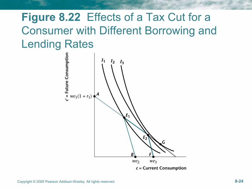
Figure 8.22 Effects of a Tax Cut for a Consumer with Different Borrowing and Lending Rates


Figure 8.23 Real Consumption of Durables, 1991–1993


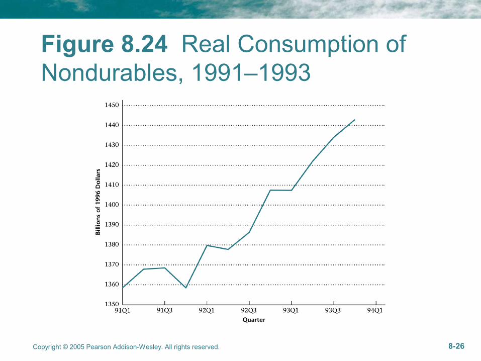
Figure 8.24 Real Consumption of Nondurables, 1991–1993


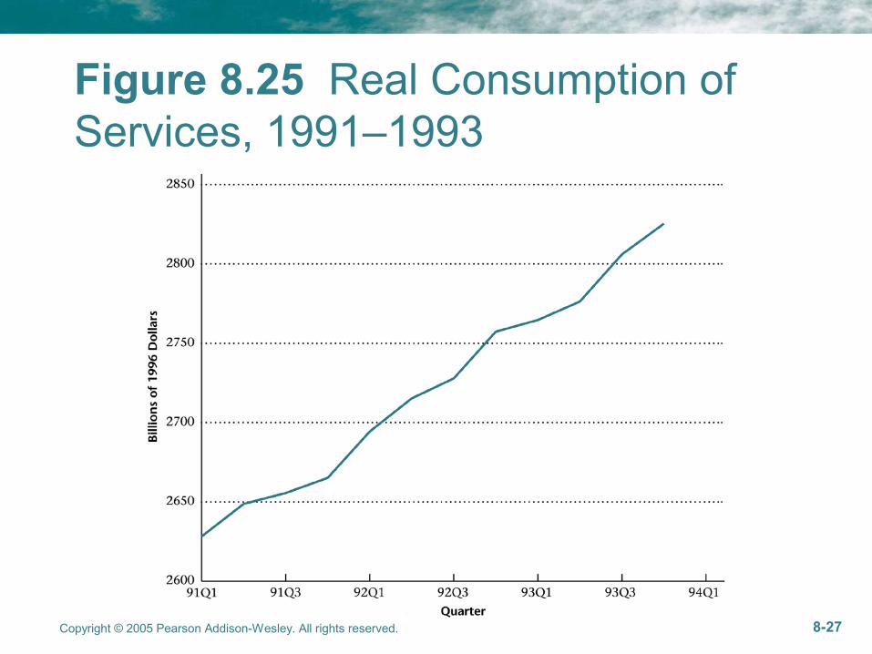
Figure 8.25 Real Consumption of Services, 1991–1993

An Extension of the Basic Model: The Life Cycle Hypothesis

• We can extend to T periods: Franco Modigliani’ life-cycle hypothesis of

consumption

• Individuals want smooth consumption profile over their life. Labor income

varies substantially over lifetime, starting out low, increasing until the

50’th year of a person’s life and then declining until 65, with no labor

income after 65.

• Life-cycle hypothesis: by saving (and borrowing) individuals turn a very

nonsmooth labor income profile into a very smooth consumption profile.

151

• Main predictions: current consumption depends on total lifetime income

and given initial wealth. as in the simple model. Saving should follow a

very pronounced life-cycle pattern with borrowing in the early periods of

an economic life, significant saving in the high earning years from 35-50

and dissaving in retirement years.

• One empirical puzzle: older household do not dissave to the extent pre-

dicted by the theory. Several explanations

1. Individuals are altruistic and want to leave bequests to their children.

2. Uncertainty with respect to length of life and health status.

152

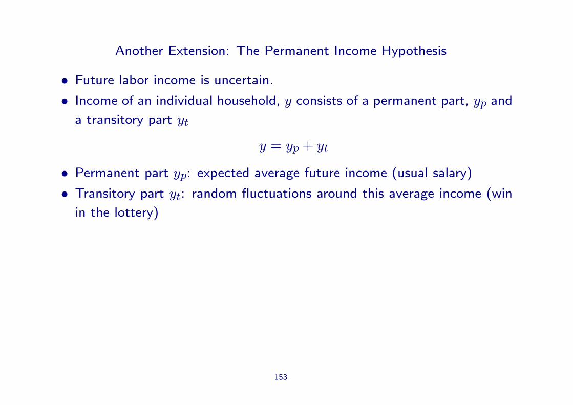
Another Extension: The Permanent Income Hypothesis

• Future labor income is uncertain.

• Income of an individual household, y consists of a permanent part, yp and

a transitory part yt

y = yp + yt

• Permanent part yp: expected average future income (usual salary)

• Transitory part yt: random fluctuations around this average income (win

in the lottery)

153

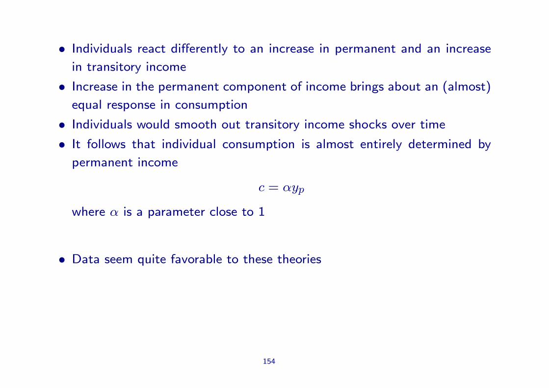
• Individuals react differently to an increase in permanent and an increase

in transitory income

• Increase in the permanent component of income brings about an (almost)

equal response in consumption

• Individuals would smooth out transitory income shocks over time

• It follows that individual consumption is almost entirely determined by

permanent income

c = αyp

where α is a parameter close to 1

• Data seem quite favorable to these theories

154

An Application of the Theory: Social Security

• Personal saving rate -the fraction of disposable income that private house-

holds save- has declined from about 7-10% in the 60’s and 70’s to 2.1%

in 1997

• Is expansion of the social security system responsible for this?

• Use simple life-cycle model to analyze this.

155

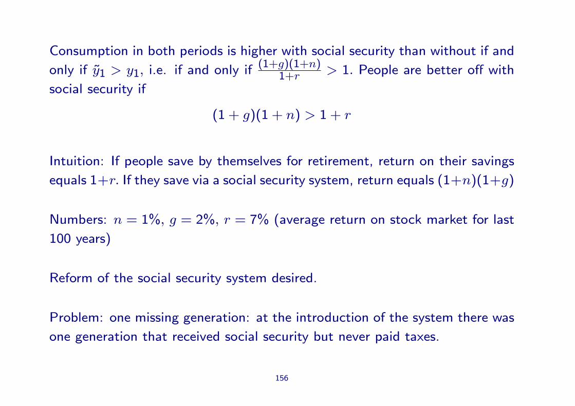
Consumption in both periods is higher with social security than without if and

only if y1 > y1, i.e. if and only if(1+g)(1+n)

1+r > 1. People are better off with

social security if

(1 + g)(1 + n) > 1 + r

Intuition: If people save by themselves for retirement, return on their savings

equals 1+r. If they save via a social security system, return equals (1+n)(1+g)

Numbers: n = 1%, g = 2%, r = 7% (average return on stock market for last

100 years)

Reform of the social security system desired.

Problem: one missing generation: at the introduction of the system there was

one generation that received social security but never paid taxes.

156

Dilemma:

1. Currently young pay double, or

2. Default on the promises for the old, or

3. Increase government debt, financed by higher taxes in the future, i.e. by

currently young and future generations

157

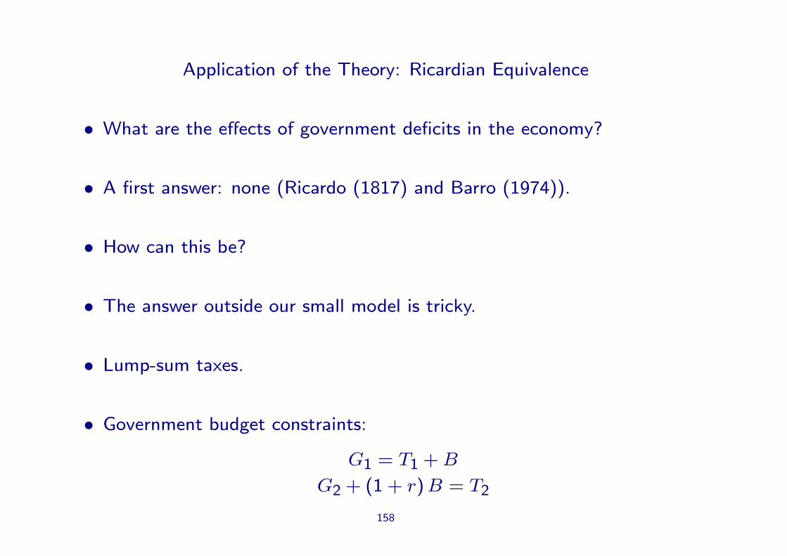
Application of the Theory: Ricardian Equivalence

• What are the effects of government deficits in the economy?

• A first answer: none (Ricardo (1817) and Barro (1974)).

• How can this be?

• The answer outside our small model is tricky.

• Lump-sum taxes.

• Government budget constraints:

G1 = T1 + B

G2 + (1 + r) B = T2

158

• Consolidating:

G1 +G2

1 + r= T1 +

T2

1 + r

• Note that r is constant (you should not worry too much about this).

159

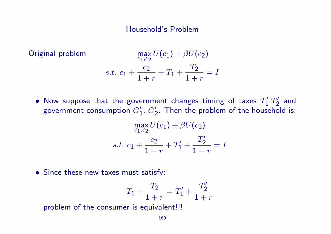
Household’s Problem

Original problem maxc1,c2

U(c1) + βU(c2)

s.t. c1 +c2

1 + r+ T1 +

T2

1 + r= I

• Now suppose that the government changes timing of taxes T ′1,T ′2 andgovernment consumption G′1, G′2. Then the problem of the household is:

maxc1,c2

U(c1) + βU(c2)

s.t. c1 +c2

1 + r+ T ′1 +

T ′21 + r

= I

• Since these new taxes must satisfy:

T1 +T2

1 + r= T ′1 +

T ′21 + r

problem of the consumer is equivalent!!!160

Empirical Evidence

• Taxes in the world are not lump-sum.

• Does the Ricardian Equivalence hold?

• Important debate.

161

Documents

12 Intertemporal Choice - School of Arts & Sciencesvr0j/econ10205/lectures/fluct...Copyright © 2005 Pearson Addison-Wesley. All rights reserved. 8-6 Figure 8.4 A Consumer Who Is a