12 Heat Loss - Chemistry, Software 8 help/12 Heat Loss.pdf · 12. Heat Loss Module The main use of this module is to estimate total heat loss or draw the temperature profile of a

HSC 8 - Heat Loss November 20, 2014

Research Center, Pori / Petri Kobylin, Peter Björklund

14008-ORC-J 1 (38)

Copyright © Outotec Oyj 2014

12. Heat Loss Module The main use of this module is to estimate total heat loss or draw the temperature profile of a wall or reactor. However, it can also be used to compare different materials and different setups, for example the use of insulation when a material has a critical maximum temperature or when the outside air cannot exceed a certain temperature. The conduction, convection and radiation databases also provide a resource as simple reference tables for material properties. Fig. 1 shows an example of a heat loss wall calculation for a smelting reactor with the temperature profile shown in rows 8 and 9.

Fig. 1. Heat Loss calculation (Heat flow) example of a smelting reactor wall.

The basic concept of the module is that the user specifies the system setup by selecting the geometry of the object, inserting columns, specifying a material for each column, specifying thicknesses (if any), and entering either one temperature point and a total heat loss or two arbitary temperature points within the same sheet. From these inputs the program can calculate either the temperature profile or the total heat loss. The temperature profile (profiles) can then be plotted graphically. The main workbook is very similar to Excel-type worksheets in terms of the properties that can be found in the menu and also most of the Excel worksheet functions are available. The new Heat Loss module may be used, for example, to estimate the heat loss values required in the Balance module. The user must first specify the column types, which can be Layer, Layer contact, Surface, and Enclosure. The thickness must be specified for the Layer and Enclosure columns, while the Layer contact and Surface columns have zero thickness. Two basic types of calculations may be carried out:



14008-ORC-J 2 (38)


1. Temperature profile with fixed heat loss and one temperature point. 2. Heat flow with two fixed temperature points. This will return the heat loss but also the

temperature profile. The calculation routine handles the conduction, convection and radiation properties as functions of temperature but fixed values may also be used by selecting the value and pressing the Fix Value button. These fixed values are shown in red on the calculation sheet. The temperature profile as well as some other user-specified values may also be presented in graphical form. The target dialog may be used to find, for example, minimum layer thickness. The calculation specifications may be saved to files for later use.



14008-ORC-J 3 (38)


12.1. Basic Calculation Procedure 1. Select geometry. To select the choice of geometry, click on the desired option button in the frame

Shape and Dimensions. The available options are wall, cube, cylinder, and sphere. It is highly recommended to start the calculations with a simple wall case and then to continue with more complicated shapes later.

2. Select dimension. When selecting the geometry, appropriate dimension textboxes will automatically pop

up. The dimensions are always inner dimensions. 3. Insert new column. The user may specify the layout of the heat transfer object by selecting Insert from

the menu bar and then the desired column type. There are four types of columns: Surface, Enclosure, Layer, and Layer contact. Surface columns must be inserted to the left and/or to the right of the other columns. Enclosure columns must be inserted between two Layer columns. Finally, the Layer contact, Enclosure, and Layer columns must all be inserted between the Surface columns.

4. Specify heat transfer type. You can select the type of heat transfer to study in two ways: either manually or using

the database.

Manually: 1. Write the name of the material/gas/liquid in the second row of the table in the current

column. 2. Select the desired heat transfer factor:

− Layer column: Enter the mean conductivity for the material (k) in row 12. − Surface column: Enter the convection and/or the radiation coefficient

(hc and/or hr) in row 13 and/or row 14. It is also possible to specify the emissivities and/or absorptivities in rows 50, 61-62, 69, in this case, please make sure that the radiation coefficient is unfixed.

− Layer contact column: Enter the thermal resistance in row 15. − Enclosure column: Enter the convection coefficient in row 13 and/or the

radiation coefficient in row 14. It is also possible to specify the emissivities in the adjacent layer columns, in this case, please make sure that the radiation coefficient is unfixed.

3. For each value entered, press the Fix Value button, unless the value is already fixed. By doing this, the program will use these given values, indicated by a red font, when calculating instead of the database values.

Using the database:

1. Press the corresponding button in the frame Get Data for Column:

− Layer column: Conduction button. − Surface column: Convection or Radiation button. − Enclosure column: Convection or Radiation button (radiation for adjacent layer

columns).



14008-ORC-J 4 (38)


− To specify the desired material/gas/liquid, place the cursor on top of it and press Select. Now the data for the material will be transferred automatically to the column on the main sheet where the cursor is located. Note that sometimes several database sheets are available, for example the convection table or function sheet. You will know that the data has been transferred from the database sheet to the calculation sheet once the selected material name appears on the material name in rows 4 or 5.

5. Specify thicknesses. Type the Thickness x in row 10 for every Layer and Enclosure column. The Surface

and Layer contact columns have zero thickness. 6. Repeat steps 3, 4, and 5 until the desired layout is achieved. 7. Calculate results. To calculate the results for a cylinder or cube, first select whether to calculate all

sheets or just the active sheet, by pressing the appropriate option button in the Calculate frame. For example, calculating only the wall sheet of a cylinder will give you the pipe calculations. The two basic calculation types are:

Temperature Profile (press the Temperature profile button):

− Specify the total heat loss by selecting the appropriate unit (W, kW or MW) and by typing the heat loss in the textbox.

− Specify one fixed temperature point with the cursor. − For cube or cylinder geometry, specify the calculation range by selecting either

Calculate all sheets (calculates all walls) or Calculate active sheet (calculates the active wall) from the option buttons.

− Note that when calculating all sheets, the temperature profiles will be iterated so that the temperatures in the first columns (inside temperatures), as well as the outside temperatures, are the same for all sheets.

Heat Flow (press the Heat flow button):

− Specify temperature points using the cursor.

− 0 or 1 point selected (by cursor position): The whole range will be calculated. • Cube or cylinder geometry: Specify calculation range by selecting either

Calculate all sheets (calculates all walls) or Calculate active sheet (calculates the active wall).

• All sheets will have the same inside and outside temperatures as in the current sheet, once the calculation is completed.

− 2 points selected (by selection): The range between these points will be calculated. • Cube or cylinder geometry: The other sheets will not be calculated. • The end temperature points in the selection will remain constant.

8. Press the Draw Diagram button for a graphical plot of the temperature profile.



14008-ORC-J 5 (38)


12.2. Heat Loss Examples

12.2.1. Examples provided by HSC See the examples provided by the HSC package by selecting File/Open from the menu and selecting the appropriate file (examples exist in the \HSC8\HeatLoss folder). 1. Simple Case with fixed conduction and convection values (SimpleCase.htr8)

In this example, the furnace wall is made of two layers, the inside temperature is 700 °C, and the outer surface is cooled with air (20 °C). The conduction and convection values are fixed. In this case, the heat flow through each layer and through the surface may easily also be calculated manually:

Firebrick: 1.5 m2 * (700 - 418 °C) * 0.4 W/(mK) / (0.23 m) = 735 W Silica brick: 1.5 m2 * (418 - 50.63 °C) * 0.2 W/(mK) / (0.15 m) = 735 W Air: 1.5 m2 * (50.63 - 20 °C) * 16 W/(m2K) = 735 W

2. Radiator heat (Radiator.htr8 file)

This example calculates the heat output of a radiator at room temperature (20 °C) and at three different water temperatures when the water flow to the radiator is zero. Select the appropriate sheet according to the inside water temperature (40 °C, 50 °C or 60 °C) and press the Heat flow button to view changes in the output heat. Adjustments can also be made to the width or length (height for a vertical wall) of the radiator to examine what influence this has on the result.

Fig. 2. Radiator calculation example.



14008-ORC-J 6 (38)


3. Heat loss from uninsulated pipe at constant T (incropera94_503.htr8 file) This is an example taken from Fundamentals of Heat and Mass Transfer by F. P. Incropera and D. P. DeWitt (page 503 in the 4th edition)1. In this example, the heat loss from an uninsulated horizontal pipe is calculated using knowledge of the surface temperature (165 °C) and air temperature (23 °C).

4. Heat loss from insulated pipe at constant T (incropera94_504.htr8 file)

Example 3 above is extended by insulating the pipe with a 25-mm thick urethane layer. Note how the heat loss decreases significantly.

5. Heat loss from a hot water tank (Hotwatertank.htr8 file)

This example is a calculation of heat loss from a hot water tank. By specifying the materials, dimensions, geometry, water, and air temperatures the total heat loss for the tank can be calculated. The insulation thickness can easily be increased separately for the top, sidewalls and bottom, in order to reduce the heat loss from the tank.

Fig. 3. Temperature profiles for a hot water tank.

6. Oil furnace (OilFurnace.htr8 file) In this example, the heat flow due to hot flue gases and internal convection in a furnace is calculated. The flue gas composition can be seen from the Gas Mixture Radiation dialog by pressing the Radiation (gas) button. The gas contains the following radiating species: H2O(g) 11.08 vol-%, CO2(g) 11.69 vol-% and SO2(g) 0.05 vol-%. This is a typical flue gas composition for fuel oils. The gas temperature is 1200 °C and the wall temperature is 500 °C. The wall surface material is “Steel (sheet with skin due to rolling)” and the convective gas is approximated as “Air (p = 1 bar)”. These can both be found in the database. There is a 10-mm thick “Plain carbon steel” layer surrounding the furnace. It is important to insert a Layer or a Layer contact



14008-ORC-J 7 (38)


column to the right of the Surface column, in order to calculate internal radiation (or convection), since the program otherwise assumes outside radiation (or convection). By entering a very low thickness value for the Layer column (row 10), or by entering zero thermal resistance for the Layer contact column (row 15), the inside surface temperature may still be used in the Layer or Layer contact column.

7. Reactor heat loss calculation (Reactor1.htr8 and Reactor2.htr8)

In this example, the total heat loss of a reactor is estimated. The given input data are the dimensions of the reactor, the surface temperature and the surrounding temperature (room temperature). The surface material in the Reactor1 example is “Steel (sheet with rough oxide layer)” and in Reactor2 “Paint, white (acrylic)”. The convective gas is “Air (p = 1 bar)” in both examples. Since the surface emissivity is lower in Reactor2, the heat loss is smaller.

8. Smelting reactor calculation (Smelting1.htr8, Smelting2.htr8 and Smelting3.htr8

files) In this example, the temperature profiles and heat losses of three different types of smelting reactors are calculated. The default input values given in this example have not been taken from any specific reactor type; however, the input values can easily be changed in order to achieve a more realistic situation.

12.2.2. Simple Step-by-Step Example (Creating Smelting1.htr8)

The following steps describe how to create the Smelting1.htr8 example from the very beginning. The final example can be used to approximate heat losses through a smelting reactor wall. The temperature profiles for different inside temperatures can be plotted using the Draw Diagram button. 1. Select File/New from the menu. 2. Select Insert/Surface column and press the Convection button. 3. From the Convection window (on the left), select the Function sheet. 4. Select Water, Copper elements cooling by moving the cursor to row 10. 5. Press the Select button. 6. Select Insert/Layer column in the main sheet and press the Conduction button. 7. Type REXAL 2S EXTRA in the yellow textbox in the Conduction window and press

Find. The cursor will now automatically move to the correct position in the database. 8. Press Select. 9. Type 1 as the layer thickness in row 10 in the main window. 10. Select Insert/Surface column and press Convection. 11. Select the Function sheet from the Convection window. 12. Select Molten metal by moving the cursor to row 4. 13. Click the Forced Convection option button and type 0.02 (= 2 cm/s) in the speed

textbox. 14. Press Select. 15. Type 1200 as the inside temperature in cell C8 and 20 as the outside temperature in

cell E9. 16. Press Heat loss.



14008-ORC-J 8 (38)


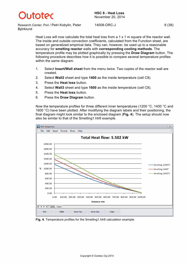
Heat Loss will now calculate the total heat loss from a 1 x 1 m square of the reactor wall. The inside and outside convection coefficients, calculated from the Function sheet, are based on generalized empirical data. They can, however, be used up to a reasonable accuracy for smelting reactor walls with corresponding cooling methods. The temperature profile may be plotted graphically by pressing the Draw Diagram button. The following procedure describes how it is possible to compare several temperature profiles within the same diagram. 1. Select Insert/Wall sheet from the menu twice. Two copies of the reactor wall are

created. 2. Select Wall2 sheet and type 1400 as the inside temperature (cell C8). 3. Press the Heat loss button. 4. Select Wall3 sheet and type 1600 as the inside temperature (cell C8). 5. Press the Heat loss button. 6. Press the Draw Diagram button. Now the temperature profiles for three different inner temperatures (1200 °C, 1400 °C and 1600 °C) have been plotted. After modifying the diagram labels and their positioning, the final diagram might look similar to the enclosed diagram (Fig. 4). The setup should now also be similar to that of the Smelting1.htr8 example.

Fig. 4. Temperature profiles for the Smelting1.htr8 calculation example.



14008-ORC-J 9 (38)


12.3. Detailed Description of the Program

12.3.1. Using the Fix Value Button and the Logic Behind It Once the Fix Value button is activated, the user is able to fix values manually to make these a direct input for the calculation. A fixed value is indicated by red font and the caption on the button changing to Unfix Value. If, for example, the user wishes to specify the convection coefficient hc directly, the specified value must be fixed (and the fluid name typed manually), otherwise the program will iterate the value using the database for the selected fluid. The program will always first look for fixed values and if the value is unfixed then it will use iterative methods and the databases. In the end, the iteration result will be returned to the cell, for example the hc value. Using fixed values significantly improves the calculation speed, although these values are not always available. As a rule of thumb, the accuracy of the result will improve if it is possible to accurately specify and fix values, for example the convection and radiation coefficients. The cells in rows 12-14 and 50, 61-62, 69 can be fixed, as well as row 15 if the column is of Layer contact type.



14008-ORC-J 10 (38)


12.3.2. Main Window

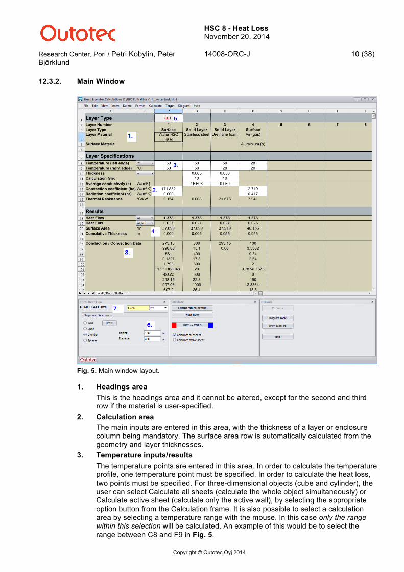
Fig. 5. Main window layout.

1. Headings area This is the headings area and it cannot be altered, except for the second and third

row if the material is user-specified. 2. Calculation area The main inputs are entered in this area, with the thickness of a layer or enclosure

column being mandatory. The surface area row is automatically calculated from the geometry and layer thicknesses.

3. Temperature inputs/results The temperature points are entered in this area. In order to calculate the temperature

profile, one temperature point must be specified. In order to calculate the heat loss, two points must be specified. For three-dimensional objects (cube and cylinder), the user can select Calculate all sheets (calculate the whole object simultaneously) or Calculate active sheet (calculate only the active wall), by selecting the appropriate option button from the Calculation frame. It is also possible to select a calculation area by selecting a temperature range with the mouse. In this case only the range within this selection will be calculated. An example of this would be to select the range between C8 and F9 in Fig. 5.



14008-ORC-J 11 (38)


4. Detailed information Here you can find more detailed information about the setup. If more precise layer

calculations are required, the Calculation grid (row 11) value may be changed. By default this is set to 10, i.e. the layer is divided into 10 elements. Note that the calculation time increases with an increasing grid size. Speed (row 38) indicates the speed of the fluid for forced convection. If this is zero, free convection is assumed. The minimum and maximum temperatures (rows 92-93) give the valid range for a certain material; N/A indicates that the limit is not available from the database. If a temperature point in the calculation result exceeds one of these points, it will be indicated by a warning message box.

5. Available data (frame) These buttons are enabled/disabled depending on the column type the cursor is placed on.

Conduction: Layer column

Convection: Surface column or Enclosure column

Radiation (surface): Surface column or Layer column (adjacent to an Enclosure column only)

Radiation (gas): Surface column, left of a Layer or Layer contact column (internal radiation)

Radiation (particles): Surface column, left of a Layer or Layer contact column (internal radiation)

6. Geometry input The option box selects the geometry and the appropriate dimension textboxes. Note

that when changing from a wall or sphere (one sheet calculations) to a cube or cylinder (one or multiple sheet calculations) the wall sheet will be copied to the adjoining sheets of the cube or cylinder. This is useful if all walls consist of the same materials, since the user only has to specify the layout of one wall and then change to the correct geometry. The Draw button draws a simple drawing of the current geometry.

7. Heat loss input/result This can be used both as input or output data. When calculating the temperature

profile, the total heat loss must be entered here, but when calculating heat loss, this can also be used as a starting approximation to achieve faster calculations. The starting approximation has a maximum value of 10 MW. If a higher value is specified, the maximum value is simply inserted in the textbox by default.

8. Radiation inputs/results Rows 96-399 consist of Convection and Conduction data and rows 400- of Radiation

data. These are automatically collected from the database sheet when pressing Select and should not be changed. You can see these rows by selecting Advanced view.



14008-ORC-J 12 (38)


12.3.3. Conduction Database

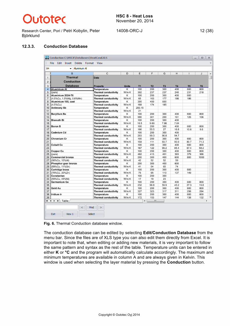
Fig. 6. Thermal Conduction database window.

The conduction database can be edited by selecting Edit/Conduction Database from the menu bar. Since the files are of XLS type you can also edit them directly from Excel. It is important to note that, when editing or adding new materials, it is very important to follow the same pattern and syntax as the rest of the table. Temperature units can be entered in either K or °C and the program will automatically calculate accordingly. The maximum and minimum temperatures are available in column A and are always given in Kelvin. This window is used when selecting the layer material by pressing the Conduction button.



14008-ORC-J 13 (38)


12.3.4. Convection Database, Table Sheet

Fig. 7. Thermal Convection database window, Table sheet.

The convection database can be edited by selecting Edit/Convection Database from the menu bar. Since the files are of XLS type you can also edit them directly from Excel. Temperature units available are K and °C. Density is not a key requirement, although it can be used in order to calculate the other properties. If the thermal expansion coefficient is not given, the program will assume that the material is an ideal gas and calculate the coefficient as β = 1/T∞. The maximum and minimum temperatures are in the hidden column A and are always given in Kelvin. This window is used when selecting the surface or enclosure material and pressing the Convection button.



14008-ORC-J 14 (38)


12.3.5. Convection Database, Function Sheet

Fig. 8. Thermal Convection database window, Function sheet.

The function sheet can be used for special cases of forced convection. For example, the Molten metal selection is an approximation of hc based on a polynomial function of the speed of the molten metal inside a smelting reactor. The database uses a function of the type hc (v) = Av^a+Bv^b+…+Gv^g where v is [m/s]. The coefficients (A-G) are located between column E and K and the exponents (a-g) in the cells directly underneath. This sheet can also be used if the convection coefficient is considered constant: simply type the constant value in column E and a zero underneath. This is shown in rows 6, 8, and 10. For a wall or cylinder it is possible to specify an angle of 0° or 90°, which means either a vertical or a horizontal object. When selecting the Forced Convection option button, a textbox for the fluid/gas speed appears under the option buttons.



14008-ORC-J 15 (38)


12.3.6. Surface Radiation Database

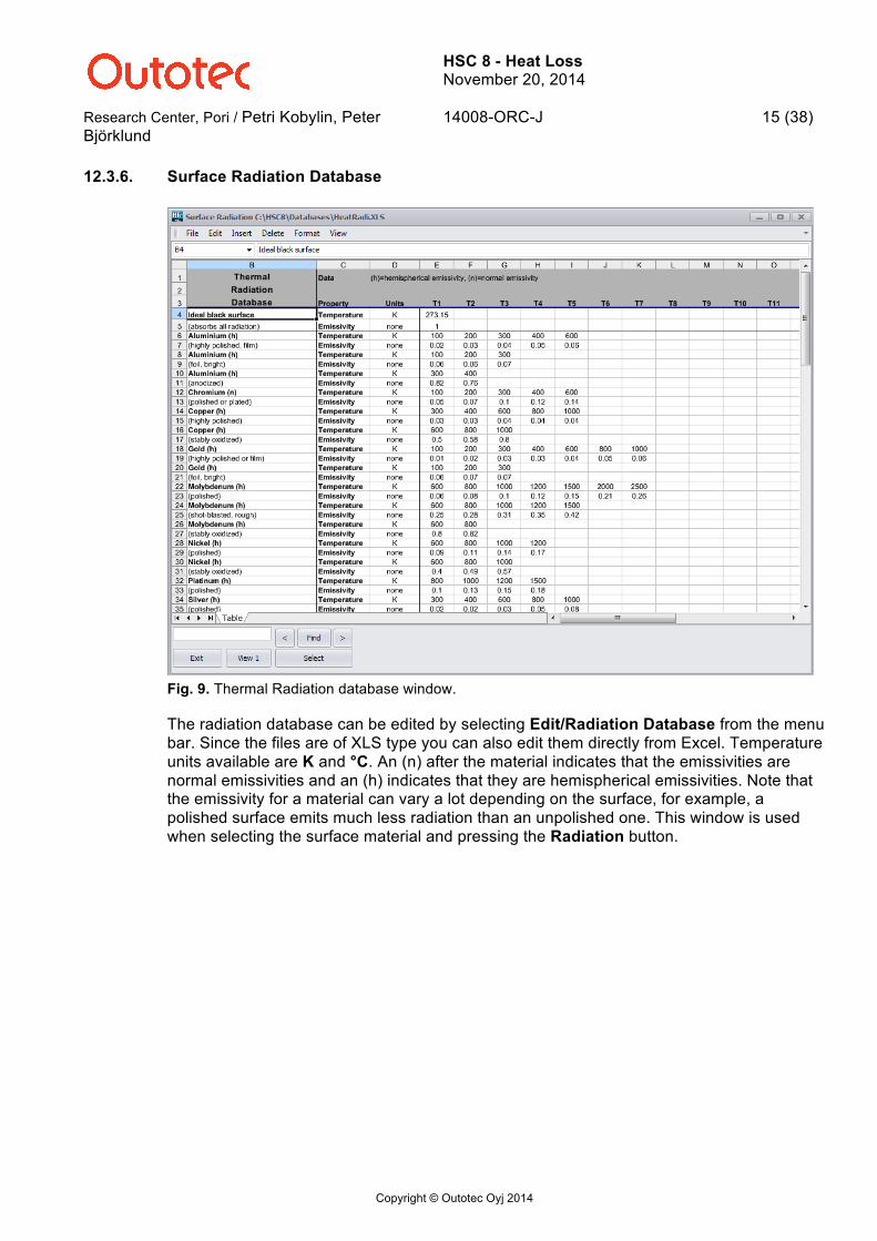
Fig. 9. Thermal Radiation database window.

The radiation database can be edited by selecting Edit/Radiation Database from the menu bar. Since the files are of XLS type you can also edit them directly from Excel. Temperature units available are K and °C. An (n) after the material indicates that the emissivities are normal emissivities and an (h) indicates that they are hemispherical emissivities. Note that the emissivity for a material can vary a lot depending on the surface, for example, a polished surface emits much less radiation than an unpolished one. This window is used when selecting the surface material and pressing the Radiation button.



14008-ORC-J 16 (38)


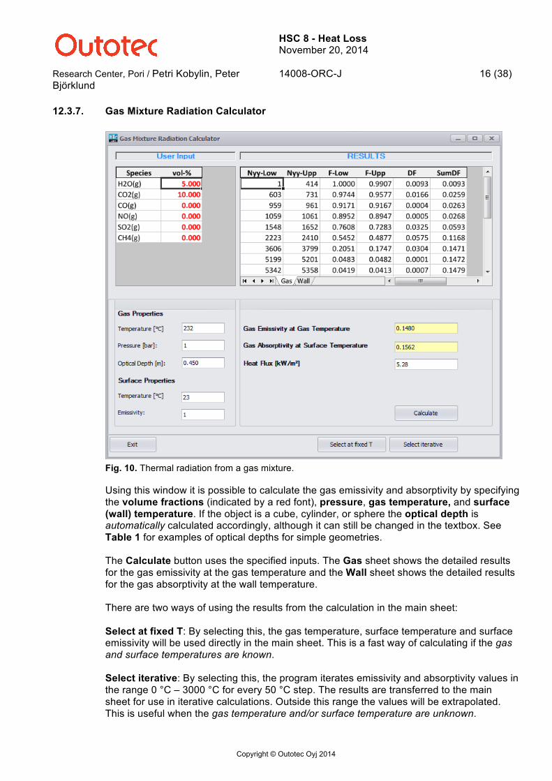
12.3.7. Gas Mixture Radiation Calculator

Fig. 10. Thermal radiation from a gas mixture.

Using this window it is possible to calculate the gas emissivity and absorptivity by specifying the volume fractions (indicated by a red font), pressure, gas temperature, and surface (wall) temperature. If the object is a cube, cylinder, or sphere the optical depth is automatically calculated accordingly, although it can still be changed in the textbox. See Table 1 for examples of optical depths for simple geometries. The Calculate button uses the specified inputs. The Gas sheet shows the detailed results for the gas emissivity at the gas temperature and the Wall sheet shows the detailed results for the gas absorptivity at the wall temperature. There are two ways of using the results from the calculation in the main sheet: Select at fixed T: By selecting this, the gas temperature, surface temperature and surface emissivity will be used directly in the main sheet. This is a fast way of calculating if the gas and surface temperatures are known. Select iterative: By selecting this, the program iterates emissivity and absorptivity values in the range 0 °C – 3000 °C for every 50 °C step. The results are transferred to the main sheet for use in iterative calculations. Outside this range the values will be extrapolated. This is useful when the gas temperature and/or surface temperature are unknown.



14008-ORC-J 17 (38)


12.3.8. Particle Radiation Calculator

Fig. 11. Particle radiation window.

Using this window it is possible to calculate a particle cloud emissivity when some detailed data about the particles and the geometry of the container are known. The results can also be used at a fixed T or iteratively as in the Gas Mixture Radiation dialog. The Diagram button shows a simple drawing of a particle distribution in a container. The gas emissivity at gas temperature and the gas absorptivity at surface temperature are automatically taken from the Gas Mixture Radiation dialog when available.



14008-ORC-J 18 (38)


12.3.9. Target Calculations (Target Dialog)

Fig. 12. Target Dialog window.

Target Dialog extends the calculation possibilities of Heat Loss. For example, it is possible to calculate the required insulation thickness to achieve a certain heat loss or, as in the example in Fig. 12, the required width of a radiator to achieve a heat loss (in this case heat output) of 0.5 kW. The following step-by-step procedure describes how Target Dialog can be used for this iteration. 1. Open the file Radiator.htr8 from the HSC8\HeatLoss directory. 2. Select Target/Target Dialog from the menu. 3. Choose Width from the drop-down box in the Variable value frame. 4. Press Set variable, which sets the width of the radiator as the variable value. 5. Choose Heat flow from the drop-down box in the Target value frame. 6. Press Set target, which sets the Heat loss of the radiator (heat output) as the target

value. 7. Choose Calculate Heat flow (calculation method) from the drop-down box in the

Iteration frame. 8. Write 1 in the Min column, 10 in the Max column, and 0.5 in the Value column. This

specifies the minimum and maximum widths and the target value for the heat loss (heat output).

9. Press Iterate Selected Rows, which calculates the required width for a heat output of 0.5 kW. The required width of the radiator is 5.747 m, as can be seen from the main window.

If the Worksheet cell option in a drop-down box is selected, any of the worksheet cells in the main window may be used as either a variable or target value. An example of this could be to iterate the required thickness of a layer (row 4) in order to achieve a certain heat loss.



14008-ORC-J 19 (38)


12.3.10. User-Specified Diagrams (Diagram Dialog) Instead of only iterating a certain target value, the Diagram Dialog may be used for graphically plotting the whole range. In the example below (Fig. 13), the influence of the inside water temperature on the heat flow (in this case the radiator heat output), is shown. The following step-by-step instructions show how this diagram can be created: 1. Open Radiator.htr8 from the HSC8\HeatLoss directory. 2. Select Diagram/Diagram Dialog from the menu. 3. Select Worksheet cell from the drop-down box in the X-value frame. 4. Move to cell C8 in the main window (inner temperature) and press Set X value in the

dialog box. 5. Select Heat flow from the drop-down box in the Y-value frame and press Set Y1

value. 6. Select Calculate Heat flow from the drop-down box in the Diagram frame. 7. Type 30 in the MIN textbox, 90 in the MAX textbox and 5 in the STEP textbox. This

means that the inner temperature will range from 30 °C to 90 °C calculated every 5 °C. The dialog box should now look similar to Fig. 13.

Fig. 13. Diagram dialog window. Specifying the diagram.

8. Press Diagram. 9. In the Diagram Table window, it is possible to specify properties in detail. However, if

this is not necessary just press Diagram here too. The resulting diagram is shown in Fig. 14.



14008-ORC-J 20 (38)


Fig. 14. Diagram showing the influence of the inside temperature on radiator heat output.

Another useful diagram would be to study the optimum insulation thickness of a cylinder geometry (for example, a pipe or a cylindrical tank). The optimal thickness is available due to an increasing outside surface area, thus increasing convective and radiative heat loss. The following step-by-step instructions show how this diagram can be created: 1. Open Hotwatertank.htr8 from the HSC8\HeatLoss directory. 2. Select Diagram/Diagram Dialog from the menu. 3. Select Worksheet cell from the drop-down box in the X-value frame. 4. Move to cell E10 in the main window (urethane insulation thickness) and press Set X

value in the dialog box. 5. Select Heat flow from the drop-down box in the Y-value frame and press Set Y1

value. 6. Select Calculate Heat flow from the drop-down box in the Diagram frame. 7. Type 0.2 in the MIN textbox, 0.5 in the MAX textbox and 0.02 in the STEP textbox.

This means that the insulation thickness varies from 0.2 m to 0.5 m and is calculated every 0.02 m.

8. Press Diagram. Note that the calculation time may be considerable on slow computers.

9. Press Diagram again in the Diagram table window. The final diagram should look similar to Fig. 15. The theoretical optimum insulation thickness is now approximately 33 cm.



14008-ORC-J 21 (38)


Fig. 15. Diagram showing the theoretical optimum sidewall insulation thickness for a cylindrical hot water tank.



14008-ORC-J 22 (38)


12.3.11. Limitations The current version of Heat Loss has some limitations, some of which are listed below.

- The maximum number of calculation sheets for a wall and a sphere is ten, for a cube four, and a cylinder three. It is also possible to insert own sheets.

- Inaccuracy increases with thick walls for a cube and cylinder, since the roof and bottom layers are “stretched” to overlap the walls. Please use surface columns only if the outer surface temperature is known, see the examples for Reactor1.htr8 and Reactor2.htr8.

- If minimum and/or maximum temperatures are not entered into the database, or directly on the sheet in rows 92 and/or 93, then the extrapolated heat transfer coefficients (k, hc and hr) may be inaccurate.

- The convection correlations are not valid for all ranges and the results cannot be trusted outside these ranges. Detailed specifications of the valid ranges are given in section 12.4.

- Inaccuracy increases with convection for small geometries.

- Forced convection cannot be used for internal calculations (gas/liquid to surface) with a cube, cylinder and sphere, since the correlations are only valid for forced external convection. Instead, the heat convection coefficient hc must be specified manually or using the Function sheet in the Conduction Database.

- If only surface columns are given for a cube, cylinder or sphere, then external convection is assumed.

- If the speed of a fluid is very low and the Table sheet is selected as input, the combined free and forced convection plays an important role; however this is not taken into account in this module.

- Radiation from a surface to the surroundings (or vice versa): the surface is considered gray and diffuse, i.e. α(T) = ε(T) only, this is however a valid approximation for most cases.

- Radiation emissivities for surfaces in the database are given as either normal (n) or hemispherical (h).

- The minimum temperature is –200 °C and the maximum is 8000 °C; however data for extreme temperatures such as these are seldom available.

- Sometimes the program is not able to iterate the answer correctly. If this happens, try using a different starting heat loss (better starting approximation) and recalculate. Make sure that the minimum or maximum temperature is not exceeded.

- When calculating temperature profiles, it is recommended to fix the outer (cooler) temperature and let the program calculate the inner temperature. The reverse selection can easily lead to temperatures lower than 0 K if the heat loss specified is too high.



14008-ORC-J 23 (38)


12.4. Basic Theory Behind Heat Transfer This chapter explains the basic theory of heat transfer used by the module. The equations and theory given are utilized within the program. The total heat flow in one dimension (x) is

Aqq xx''= (1)

where ''

xq is the heat flux and A is the unit area. It is often practical to use an analogy between heat transfer and Ohm’s law in electricity. The thermal resistance is defined as

xqTTR 21 −= , (2)

where T1 and T2 are the temperature points and qx is the heat flow. The thermal conductance is then

RG 1= , (3)

where R is the thermal resistance. Time-dependent heat flows, where qx = q(x, t), and steady-state non-time-dependent heat flows qx = q(x) are two basic ways of identifying heat transfer problems. This program is concerned only with steady-state non-time-dependent conditions, which means that the condition is valid for infinite t. A number of dimensionless parameters are used in this chapter. Some of them are only material-specific and can be listed in a table, while others are geometry-specific or directly related. Equations (4) to (7) show the most important ones. The thermal diffusivity is defined as

ρα

pck

= , (4)

where k is the thermal conductivity, cp is the heat capacity at constant pressure, and r is the density. The kinematic viscosity is defined as

ρµ

ν = , (5)

where µ is the dynamic viscosity. The Prandtl number describes the ratio of momentum and thermal diffusivities. This is defined as



14008-ORC-J 24 (38)


αν

=Pr , (6)

where ν is the kinematic viscosity and α is the thermal diffusivity. The thermal expansion coefficient is defined as

TT p ΔΔ

−≈⎟⎠

⎞⎜⎝

⎛∂∂

−=ρ

ρρ

ρβ

11, (7)

where p denotes the derivative at constant pressure. When calculating the heat flux, it must be separated into the three main forms: conduction, convection, and radiation. A more detailed description of these forms will be given in the following sections.



14008-ORC-J 25 (38)


12.4.1. Conduction Heat transfer due to conduction occurs between points inside a material or materials connected to each other. Thermal conductivity is very dependent on the phase the material is in and on the temperature of the material/materials. Therefore, accurate calculations with a simple non-iterative formula are sometimes impossible. The use of a numerical technique such as an element method can be applied in order to achieve more accurate results. The conduction heat flux for one dimension (Fourier’s law) is calculated as

dxdTkqx −='' , (8)

where dT/dx is the temperature derivative in x-direction. The function k = k(T) is generally not expressed the same way as the heat capacity function cp = cp(T), which is a fitted equation in other parts of HSC, i.e. the Kelley equation. Instead, the values of k are known at certain temperature points and linear interpolation and extrapolation may be used for temperatures outside these points. When calculating the heat flux (or flow) the distance between the two temperature points is divided into a grid. Hence, the heat flux can be calculated by using the following approximate equation that calculates the average heat flux through a layer:

( )

∑

∑

=

−+=

Δ⋅

−⋅−= m

nn

nn

m

nn

x

xm

TTkq

1

2/12/11'' , (9)

where kn = kn (Tn) is the heat conduction coefficient at Tn (middle of the grid), m is a grid step (the amount of steps distance x is divided into), n is the point in the middle of one grid step, Tn+1/2 is the temperature point between grid n and grid n+1, Tn-1/2 is the temperature point between grid n and grid n-1, and Δxn is the thickness of the grid. In order to be able to calculate other geometries, the shape factor S in the total heat rate equation TSkAqq x Δ== '' is defined for different geometries according to Eqs (10) to (12). For one-dimensional plane walls and cube walls (10), cylindrical walls (11) (cylindrical coordinates) and spherical walls (12) (spherical coordinates), S is defined respectively as

xAS /= , (10)

( )io xxhS/ln

2π= , (11)

io

oi

xxxxS

−=

π4 . (12)

where A is the unit area for the layer and x is the thickness of the layer. h is the height of the cylinder and xo, xi are the outer and the inner radius of the layer.



14008-ORC-J 26 (38)


12.4.2. Convection Heat transfer due to convection occurs between two points, where one is on a surface and the other in a fluid/gas. Convection cannot normally be solved mathematically except for some laminar cases. Therefore, convection calculations are mostly based on empirical equations or correlations and the uncertainty, or margin of error in these calculations can be as high as ±20%. In the literature, these correlations can also vary and the validity of the result is mostly limited to some range of one or more thermophysical properties of the fluid/gas. The correlation equations used in the program are taken from1,2. The heat flux due to convection is calculated as

( )∞−= TThq sc'' , (13) where hc is the convection coefficient, Ts is the surface temperature, and T∞ is the fluid/gas temperature. The mathematical models for hc, based on experimental data, are given in dimensionless form using the Nusselt number, which is defined as

kLhNu c

L = , (14)

where L is the characteristic length for the prescribed geometry. The Nusselt number can be related through empirical data to other properties of the convective gas/fluid. These properties are normally temperature- and pressure-dependent, hence the film temperature, Tf = (Ts+T∞)/2, should be used when determining these properties. The task is then simply to describe the problem as accurately as possible and to select the appropriate correlation. Using Equation (14) and the appropriate correlation equation, the value of hc can be calculated. The correlations depend on whether forced or free (natural) convection is studied. In forced convection, the motion of the fluid is due to an external pressure gradient caused by a fan or a pump. In free convection the fluid motion is due to buoyancy forces only, such as gravitational or centrifugal forces. In some forced convection cases when the speed of the fluid is low, there is a mixture of forced and free convection called mixed convection, however this is not taken into account in this work. See 12.3.11 Limitations for a more detailed description of when mixed convection conditions are noticeable. Convection can also be subdivided into an internal and external flow, which means that the fluid is either contained inside an enclosure or flowing freely outside a geometry. Flow in pipes is an example of a forced internal flow that has been studied thoroughly. Forced internal flow is more difficult to examine due to, for instance, the influence of centrifugal forces inside reactors. The convection coefficient is also dependent on the way the fluid is put into motion, for example, different types of propellers give different coefficients. In some cases, simple experimental correlations for the convection coefficient in the form hc = hc(u∞) may be used. External flow has also been studied extensively and listed below are the different correlations that may be used for different cases. Note that for a plane wall the internal convection is equivalent to the external convection.



14008-ORC-J 27 (38)


Free Convection The correlation describing the nature of the flow for free convection is called the Rayleigh number and is defined according to

ναβ 3)( LTTgRa s

L∞−

= , (15)

where g is the acceleration due to gravity and β the thermal expansion coefficient. Sometimes the Grashof number, which describes the ratio of buoyancy forces to viscous forces, is used in correlations and is defined as

Pr)(

2

3Ls

LRaLTTgGr =

−= ∞

νβ . (16)

A description of how to calculate the free convection Nusselt number, defined in equation 14, for different geometries is explained below. Wall, vertical position1 θv = 0°: Surface:

• Characteristic length: L = z • Laminar flow (RaL < 109):

( )[ ] 9/416/9

4/1

Pr/492.01

670.068.0+

+= LL

RaNu (17)

• Turbulent flow (RaL ≥ 109):

[ ]

2

27/816/9

6/1

Pr)/492.0(1

387.0825.0⎪⎭

⎪⎬⎫

⎪⎩

⎪⎨⎧

++= L

LRaNu (18)

Enclosure:

• Characteristic length: L = thickness of wall enclosure • H = z (height of enclosure) • H/L ≤ 2:

29.0

Pr2.0Pr18.0 ⎟

⎠

⎞⎜⎝

⎛+

= LL RaNu (19)

• Valid when:

1 < H/L < 2 10-3 < Pr < 105

103 < (RaLPr)/(0.2+Pr)

• 2 < H/L < 10:

4/128.0

Pr2.0Pr22.0

−

⎟⎠

⎞⎜⎝

⎛⎟⎠

⎞⎜⎝

⎛+

=LHRaNu LL (20)



14008-ORC-J 28 (38)


• Valid when: 2 < H/L < 10 Pr < 105 103 < RaL < 1010

• H/L ≥ 10:

3.0012.04/1 Pr42.0

−

⎟⎠

⎞⎜⎝

⎛=

LHRaNu LL (21)

• Valid when:

10 < H/L < 40 1 < Pr < 2·104 104 < RaL < 107

Wall, horizontal position1,2 θv = 90°: Surface:

• Characteristic length: L = A/P, i.e. the surface area divided by the perimeter Hot upper surface or cold lower surface:

4/127.0 LL RaNu = (22) Cold upper surface or hot upper surface:

• RaL < 107:

4/154.0 LL RaNu = (23)

• RaL ≥ 107:

3/115.0 LL RaNu = (24) Enclosure:

• Characteristic length: L = thickness of wall enclosure • Hot lower surface: • RaL ≤ 1708:

1=LNu (pure conduction) • RaL > 1708:

074.03/1 Pr069.0 LL RaNu = (25)

• Valid when:

3·105 < RaL < 7·109

• Cold lower surface:

1=LNu (pure conduction)

Cube1: Surface:

Internal flow:



14008-ORC-J 29 (38)


• Characteristic length: L = zi • Nusselt number according to Equation (17) or (18) for all walls • The flow is assumed to cool down at the walls (downflow), thus creating a

circulating flow with an upflow through the center of the cube. • Not valid for small cubes

External flow:

Cube walls:

• Characteristic length: L = zo • Nusselt number according to Equation (17) or (18)

Roof and bottom:

• Characteristic length: L = A/P, i.e. the roof/bottom surface area divided by the perimeter

• Nuroof and Nubottom according to Equation (22), (23) or (24) Enclosure:

• Same as for wall depending on horizontal or vertical cube enclosure

Cylinder, vertical1 θv = 0°: Surface:

Internal flow: • Characteristic length: L = zi • Nusselt number according to Equation (17) or (18) for wall, roof and bottom • The flow is assumed to cool down at the walls (downflow), thus creating a

circulating flow with an upflow through the center of the cylinder • Not valid for small cylinders

External flow:

Cylinder wall:

• Characteristic length: L = zo • Nusselt number according to Equation (17) or (18)

• Valid when: 4/1Pr)//(35/ LRaLD ≥

Roof and bottom:

• Characteristic length: L = A/P = D/4, i.e. the surface area divided by the perimeter

• Nuwall according to Equation (17) or (18) • Nuroof and Nubottom according to Equation (22), (23) or (24)

Enclosure:

• Approximated as vertical wall enclosure

Cylinder, horizontal1 θv = 90°: Surface:

Internal flow:

• Characteristic length: L = Di • Nusselt number calculated according to Equation (17) or (18)



14008-ORC-J 30 (38)


• The flow is assumed to cool down at the walls (downflow), thus creating a circulating flow with an upflow through the center of the cylinder

• Not valid for small cylinders

External flow:

Cylinder wall:

• Characteristic length: L = Do

[ ]

2

27/816/9

6/1

Pr)/559.0(1

387.060.0⎪⎭

⎪⎬⎫

⎪⎩

⎪⎨⎧

++= D

DRaNu (26)

• Valid when:

RaD ≤ 1012

Roof and bottom: • Characteristic length: πorL = , i.e. square with same area • Nuroof and Nubottom according to Equation (17) or (18)

Enclosure:

• Characteristic length L = thickness of cylinder enclosure • hc calculated directly, not through the Nusselt number (NuL)

( )[ ]( ) L

oi

ioc Ra

DDL

DDRa 55/35/33

4* /ln

−− += (27)

• Rac

* < 100:

( ) 2//ln iioc DDD

kh⋅

= (28)

• Rac

* ≥ 100:

( ) kRak ceff ⋅⎟⎠

⎞⎜⎝

⎛+

=4/1*

4/1

Pr861.0Pr386.0 (29)

( ) 2//ln iio

effc DDD

kh⋅

= (30)

• valid when:

102 ≤ Rac* ≤ 107

Sphere /1/: Surface:

Internal flow:

• Characteristic length: L = zi • Nusselt number according to Equation (17) or (18) • The flow is assumed to cool down at the walls (downflow), thus creating a

circulating flow with an upflow through the center of the sphere • Not valid for small spheres



14008-ORC-J 31 (38)


External flow:


[ ] 9/416/9

4/1

Pr)/469.0(1

589.02+

+= DD

RaNu (31)

• Valid when:

RaD ≤ 1011 Pr ≥ 0.7

Enclosure: • Characteristic length: L = thickness of the sphere enclosure • hc calculated directly, not through the Nusselt number (NuL)

( ) ( )55/75/74*

−− +=

oi

L

ios

DD

RaDDLRa (32)

• Ras

* < 100:

LDDkh oi

c π= (33)

• Ras

* ≥ 100:

( ) kRak seff ⋅⎟⎠

⎞⎜⎝

⎛+

=4/1*

4/1

Pr861.0Pr74.0 (34)

LDDkh oi

effc π= (35)

• Valid when: 102 ≤ Ras

* ≤ 104



14008-ORC-J 32 (38)


Forced Convection Forced convection is here assumed to be external only. The correlation number describing the nature of the flow for forced convection is called the Reynolds number, which describes the ratio of inertia forces to viscous forces of a flow and is defined as

νLu

L∞=Re (36)

where u∞ is the speed of the fluid/gas. Note that the direction of the flow is assumed to be horizontal in this program and that forced convection inside enclosures is not taken into consideration. Wall1:

• Laminar flow, ReL ≤ 5·105:

3/12/1 PrRe664.0 LLNu = (37)

• Valid when: Pr ≥ 0.6

• Turbulent flow (flow separation), ReL ≥ 5·105:

3/15/4 Pr)871Re037.0( −= LLNu (38)

• Valid when: 0.6 ≤ Pr ≤ 60

5·105 ≤ ReL ≤ 108 Cube1:

• Tangential horizontal flow on all sides assumed Cube walls:

• Characteristic length front and back wall: L = xo

• Characteristic length left and right wall: L = yo

• Nusselt number calculated as (37) or (38)

Roof and bottom:

• Characteristic length: L = yo • Nusselt number calculated as (37) or (38)

Cylinder1:

Cylinder wall:




14008-ORC-J 33 (38)


( )[ ]5/48/5

4/13/2

3/12/1

282000Re1

Pr/4.01

PrRe62.03.0⎥⎥⎦

⎤

⎢⎢⎣

⎡⎟⎠

⎞⎜⎝

⎛+

++= DD

DNu (39)

• Valid when:

ReD·Pr ≥ 0.2

Roof and bottom: • Characteristic length: πorL = , i.e. square with same area • Nusselt number calculated as (37) or (38)

Sphere1,2:


4/14.03/22/1 Pr)Re06.0Re4.0(2 ⎟⎟

⎠

⎞⎜⎜⎝

⎛++= ∞

sDDDNu

µµ

, (40)

where μ

∞ is the dynamic viscosity at the fluid/gas temperature and μs is the dynamic

viscosity at the surface temperature.

• valid when: 0.71 ≤ Pr ≤ 380 3.5 ≤ ReD ≤ 7.6·104 1.0 ≤ (μ∞/μs) ≤ 3.2



14008-ORC-J 34 (38)


12.4.3. Radiation Heat transfer due to radiation occurs in the range of approximately 0.4 mm to 1000 mm of the electromagnetic wavelength spectrum3. This spectrum includes both visible light as well as infrared radiation. Radiation heat transfer between two points occurs when waves are emitted at one point and absorbed at another. Sometimes the wave is reflected or transmitted and thus there is no radiation heat transfer between these two points. However, the wave can be absorbed at another point thus creating a heat flow between these new points instead. Since radiation consists of electromagnetic waves, it is therefore not dependent on the medium; in fact radiation heat transfer through a vacuum is higher than through other media since almost no radiation is absorbed there. Radiation plays a significant role at high temperatures and radiation heat transfer is in this instance much higher than convection heat transfer. This can be seen from Equations (41), (44) and (52), with temperatures raised to the power of four. Radiation heat transfer can be subdivided into three types: Surface radiation, gas radiation, and combined gas and particle radiation. These are described in more detail below. Surface Radiation Surface radiation means that the heat flux is due to a surface (at temperature Ts) that radiates to the outside environment (at temperature T∞), which is assumed to be very large compared to the radiating surface. A typical case could be the walls of a big room. The net heat flux is calculated according to

( )44'' ∞−= TTq ssσε , (41) where εs is the surface emissivity, which is a function of the surface temperature, εs = εs(Ts) and σ is the Stefan-Boltzmann constant. The surface is assumed to be gray, which means that the surface absorptivity is equal to the surface emissivity: (αs(T) = εs(T)). For easier comparison with the convection heat rate, we can define the heat radiation coefficient as

( )( )22∞∞ ++= TTTTh sssr σε (42)

and by using equations (41) and (42), the heat rate can be expressed as

( )∞−= TThq sr'' , (43) which is in the same form as Equation (13). The surface emissivity can be found from tables in the literature. The normal emissivity (εn) or the hemispherical or total emissivity (εh) may be listed depending on the material. The normal emissivity is the normal directional emissivity while the hemispherical emissivity is the averaged value for all solid angles passing through a hemisphere centered over the surface element3.



14008-ORC-J 35 (38)


Gas Radiation The heat flux due to radiation from a gas to a surface is calculated as4

( )44

21'' sggg

s TTq αεσε

−+

= , (44)

where εs is the surface emissivity, εg = εg(Tg) is the gas emissivity at the gas temperature, and αg = αg(Tg,Ts) is the gas absorptivity as a function of both the gas and surface temperatures. It is natural that αg also depends on Ts, as this defines the spectrum of incoming radiation. This is clear because Tg defines the state of the gas and therefore its thermal properties. The surface is also here assumed to be gray. The coefficient (εs+1)/2 is an approximation for the effective emissivity of the solid. The heat radiation coefficient is now

( ) ( )( )sg

sgggsr TT

TTh

−

−+=

21 44 αεσε

. (45)

In order to calculate εg and αg, the exponential wide band model5 can be used. This model has been optimized and made more efficient computationally6. The model can treat mixtures containing H2O, CO2, CO, NO, SO2, and CH4 in, for example, a non-radiating nitrogen gas. The model also takes into account the pressure and the optical depth of the geometry. The gas emissivity function is

),,,,,,,,( 4222 CHSONOCOCOOHggg xxxxxxLpTεε = , (46) where p is the pressure, L is the optical depth, and x is the molar fraction of the individual gas species. Note that the sum of the radiating gases can be smaller than one, Σxsp ≤ 1, since the rest of the mixture can consist of non-radiating gases. This model is applicable for the temperature range T = 300 K to 2500-3000 K and the pressure range p = 0.5 to 20 bar. The optical depth L depends on the geometry and is listed in the following table for the most common geometries7. All surfaces are assumed to be able to absorb radiation. Table 1. Examples of optical depths for simple geometries

Geometry Characteristic dimension Optical depth (L) 1. Sphere Diameter (D) 0.63D 2.1 Cylinder (h = 0.5D) Diameter (D) 0.45D 2.2 Cylinder (h = D) Diameter (D) 0.6D 2.3 Cylinder (h = 2D) Diameter (D) 0.73D 3.1 Cube (1x1x1) Any side (x) 0.6x 3.2 Cube (1x1x4) Shortest side (x) 0.81x 3.3 Cube (1x2x6) Shortest side (x) 1.06x



14008-ORC-J 36 (38)


For dimensions not listed in Table 1, the optical depth coefficient can be interpolated or extrapolated. A simple example is: Calculate the optical depth for a cube with the dimensions 1x4x7. 1. Extrapolated as a 1x1x7 cube using geometries 3.1 and 3.2 gives L1x1x7 = 0.6+(0.81-0.6)·[(7-1)/(4-1)] = 1.02

2. Extrapolated as a 1x2.5x7 cube using geometries 3.2 and 3.3 gives L1x2.5x7 = 0.81+(1.06-0.81)·[(2.5-1)/(2-1)] = 1.185.

3. These two results can then be used again to extrapolate to the 1x4x7 cube, which gives L1x4x7 = 1.02+(1.185-1.02)·[(4-1)/(2.5-1)] = 1.35. This is the answer since the shortest side is x = 1.

The gas absorptivity at the surface temperature can be calculated using the same model if two temperature correction factors are introduced. The function then becomes

5.0

4222

5.1

),,,,,,,,( ⎟⎟⎠

⎞⎜⎜⎝

⎛⋅⎟

⎟⎠

⎞⎜⎜⎝

⎛⋅=

s

gCHSONOCOCOOH

g

sggg T

Txxxxxx

TTLpTεα (47)

and as seen from the correction factors, the surface temperature Ts is now also needed as an input. For further information and detail on this model5,6. The gas radiation calculation code used by HSC is based on code made by Tapio Ahokainen. Combined Gas and Particle Radiation Particle cloud emissivity can be calculated when the mean size of the particles and the particle cloud geometry are known, according to4

ppp LAnc e εε −−=1 , (48)

where εp is the emissivity of a single particle, np is the number of particles per unit volume of cloud, L is the thickness of the cloud, and Ap is the average cross-sectional area of the particle. If the particles in the cloud are not uniform in size, then the surface mean diameter can be used according to

∑

∑

=

=== n

ii

n

iii

s

n

dndA

1

1

22

44ππ , (49)

where ds is the surface mean diameter and ni is the number of particles of the same diameter di . The total gas and particle cloud emissivity can then be approximated as7

cgcgcg εεεεε −+=+ , (50) where εc is the particle cloud emissivity and εg is the gas emissivity calculated according to the model behind Equation (46). The total gas and particle cloud absorptivity can be approximated as



14008-ORC-J 37 (38)


cgcgcg εαεαα −+=+ , (51) where αg is the gas absorptivity calculated according to the model behind Equation (47). Finally, the heat flux due to radiation from a gas and particle cloud to a surface is then calculated according to7

( )44'' scggcgscgscg

s TTq ++++

−−+

= αεσεαεα

ε (52)

and the heat radiation coefficient as

( )( )( )sgscgscg

scggcgsr TT

TTh

−−+

−=

++

++

εαεα

αεσε 44

(53)



14008-ORC-J 38 (38)


12.5. References 1. Incropera, F.P. & DeWitt, D.P.: Fundamentals of Heat and Mass Transfer, Fourth

Edition. John Wiley & Sons, New York, 1996. ISBN 0-471-30460-3. 2. Taine J. & Petit J-P.: Heat Transfer. Prentice Hall, Hempstead, 1993. ISBN 0-13-

387994-1. 3. Siegel R. & Howell J.R.: Thermal Radiation Heat Transfer, Second Edition.

Hemisphere Publishing Corporation, 1972. ISBN 0-07-057316-6. 4. Themelis N.J.: Transport and Chemical Rate Phenomena. Gordon and Breach

Science Publishers SA, 1995. ISBN 2-88449-127-9. 5. Edwards, D.K., Balakrishnan A. Thermal Radiation by Combustion Gases. Int. J. Heat

Mass Transfer, vol. 16, pp. 25-40, 1973. 6. Lallemant N. & Weber R.: A computationally efficient procedure for calculating gas

radiative properties using the exponential wide band model. Int. J. Heat Mass Transfer, vol. 39, No.15, pp. 3273-3286, 1996.

7. VDI Heat Atlas. Düsseldorf VDI-Verlag, 1993. 8. Haar L. & Gallagher J.S. & Kell G.S.: NBS/NRC Steam Tables: Thermodynamic and

Transport Properties and Computer Programs for Vapor and Liquid States of Water in SI Units. Hemisphere Publishing Corporation, 1984. ISBN 0-89116-353-0.

9. Jokilaakso A.: Virtaustekniikan, lämmönsiirron ja aineensiirron perusteet. Technical University of Helsinki, Otakustantamo, 1987. ISBN 951-672-015-3.

10. Edwards, D.K. Gas radiation properties. Heat Exchanger Design Handbook, No. 5 Physical Properties. VDI-Verlag GmbH, Hemisphere Publishing Corp. 1983 (approx. 250 p.)

Documents

12 Heat Loss - Chemistry, Software 8 help/12 Heat Loss.pdf · 12. Heat Loss Module The main use of this module is to estimate total heat loss or draw the temperature profile of a