Embed Size (px)
Citation preview
Copper Case Study Draft Nov 2011 Memary et al 1
figure
CLUSTER RESEARCH
REPORT No. 1.12
Prepared by:
Department of Civil Engineering, Monash University Institute for Sustainable Futures, University of Technology, Sydney
For CSIRO Minerals Down Under National Research Flagship
Future Greenhouse Gas Emissions from Copper Mining: Assessing Clean Energy Scenarios
G.M. Mudd, Weng, Z., R. Memary, S.A. Northey,D. Giurco, S. Mohr, L. Mason
October 2012
ABOUT THE AUTHORS
Department of Civil Engineering: Monash University The Department of Civil Engineering, within the Faculty of Engineering at Monash University aims to provide high quality Civil Engineering education, research and professional services globally for the mutual benefit of the students, the staff, the University, industry, the profession and the wider community
For further information visit www.eng.monash.edu.au/civil/
Research team:
Dr Gavin M. Mudd, Senior Lecturer; Mr Zehan Weng, Research Assistant; Mr Stephen A. Northey, Research Assistant
Institute for Sustainable Futures: University of Technology, Sydney The Institute for Sustainable Futures (ISF) was established by the University of Technology, Sydney in 1996 to work with industry, government and the community to develop sustainable futures through research and consultancy. Our mission is to create change toward sustainable futures that protect and enhance the environment, human well‐being and social equity. We seek to adopt an inter‐disciplinary approach to our work and engage our partner organisations in a collaborative process that emphasises strategic decision making.
For further information visit www.isf.uts.edu.au
Research team:
Mr Reza Memary, Research Assistant; Dr Steve Mohr, Senior Research Consultant; Ms Leah Mason, Senior Research Consultant; Dr Damien Giurco, Research Director.
CITATION Cite this report as:
Mudd, G.M., Weng, Z., Memary, R., Northey, S. A., Giurco, D., Mohr, S., and Mason, L. (2012) Future greenhouse gas emissions from copper mining: assessing clean energy scenarios. Prepared for CSIRO Minerals Down Under Flagship by Monash University and Institute for Sustainable Futures, UTS. ISBN 978‐1‐922173‐48‐5.
ACKNOWLEDGEMENT This research has been undertaken as part of the Minerals Futures Research Cluster, a collaborative program between the Australian CSIRO (Commonwealth Scientific Industrial Research Organisation); The University of Queensland; The University of Technology, Sydney; Curtin University; CQUniversity; and The Australian National University. The authors gratefully acknowledge the contribution of each partner and the CSIRO Flagship Collaboration Fund. The Minerals Futures Cluster is a part of the Minerals Down Under National Research Flagship, http://www.csiro.au/Organisation‐Structure/Flagships/Minerals‐Down‐Under‐Flagship/mineral‐futures‐collaboration‐cluster.aspx.
EXECUTIVE SUMMARY This report is submitted as part of the Commodity Futures component of the Mineral
Futures Collaboration Cluster as a case study on copper. This report covers the case study
on copper mining and smelting in Australia with a critical reflection on future environmental
and technological challenges facing the copper related mining and mineral industries of
Australia. A key focus is detailed life cycle assessment (LCA) modelling of the greenhouse gas
emissions intensity of future copper mining and milling, based on a detailed copper resource
data set.
In this study, we focussed on analysing the likely future environmental footprint of primary
copper supply, rather than how to meet copper demand. We develop a peak copper
production model, based on a detailed copper resource data set, and combine this with a
comprehensive life cycle assessment model of copper mining and milling to predict
greenhouse gas emission rates and intensities of Australian and global copper production up
to 2100. By establishing a quantitative prediction of both copper production and
corresponding greenhouse gas emissions of Australian and global copper industry, we then
analysed the emissions intensity of various energy input scenarios, such as business‐as‐
usual, solar thermal electricity and solar thermal electricity with biodiesel.
The Australian Government has an aspirational goal long‐term greenhouse gas emissions of
an 80% reduction from the 2000 level by 2050. For the copper sector, this means moving
from about 12.6 Mt CO2e in 2000 to a goal of some 2.52 Mt CO2e in 2050 (assuming equal
emissions reductions across the economy). Based on the energy sources modelled, only the
solar thermal plus biodiesel scenario was capable of achieving this goal at about 0.15 Mt
CO2e, since the solar thermal alone scenario still includes normal petro‐diesel as a major
source of emissions.
Overall, it is clear that there are abundant resources which can meet expected long‐term
copper demands, the critical issue is more the environmental footprint of different copper
supplies and use rather than how much is available for mining. It is clear that the switch to
renewable energy can have a profound impact on the carbon intensity of copper supply and
a complete conversion to renewable energy will position the copper sector to meet existing
annual greenhouse gas emissions targets and goals.
1
Contents1. BACKGROUND..................................................................................................................... 2
1.1. Aim .............................................................................................................................. 2
2. Brief Review of Copper Mining and Demand ..................................................................... 3
2.1. Global copper production ........................................................................................... 3
2.2. Copper demand ........................................................................................................... 5
3. Climate Change Impacts of Copper Mining ........................................................................ 8
3.1. Life cycle assessment of copper production ............................................................... 8
3.2. Energy inputs into mining stages ................................................................................ 8
3.3. Relationship between ore grade and carbon intensity of final product ..................... 9
4. Methodology .................................................................................................................... 10
4.1. Peak modelling of future copper production ............................................................ 10
4.2. LCA model of copper mining ..................................................................................... 13
4.3. Copper production and ore grade projections ......................................................... 15
5. Results ............................................................................................................................... 16
5.1. Greenhouse gas emissions projections of global copper mining ............................. 16
5.2. Greenhouse gas emissions projections of Australian copper mining ....................... 16
6. Analysis & Discussion ........................................................................................................ 20
6.1. Greenhouse gas emissions targets and trajectories ................................................. 20
6.2. Implications for the future of copper........................................................................ 22
7. Conclusion ........................................................................................................................ 24
8. References ........................................................................................................................ 25
9. Appendix 1 ........................................................................................................................ 28
2
1. BACKGROUND
This report is submitted as part of the Commodity Futures component of the Mineral
Futures Collaboration Cluster as a case study on copper. The commodity futures project
focuses on the macro‐scale challenges, the dynamics, and drivers of change facing the
Australian minerals industry. The Commodity Futures project aims to:
Explore plausible and preferable future scenarios for the Australian minerals industry
that maximise national benefit in the coming 30 to 50 years
Identify strategies for improved resource governance for sustainability across scales,
from regional to national and international
Establish a detailed understanding of the dynamics of peak minerals in Australia, with
regional, national and international implications
Develop strategies to maximise value from mineral wealth over generations, including an
analysis of Australia’s long‐term competitiveness for specified minerals post‐peak.
This report covers the case study on copper mining and smelting in Australia with a critical
reflection on future environmental and technological challenges facing the copper related
mining and mineral industries of Australia. A key focus is detailed life cycle assessment (LCA)
modelling of the greenhouse gas emissions intensity of future copper mining and milling,
based on a detailed copper resource data set.
1.1. Aim The aim of this paper is to review the link between resources, technology and changing
environmental impacts over time as a basis for informing future research priorities in
technology and resource governance models.
3
2. Brief Review of Copper Mining and Demand Copper’s characteristics such as ductility, malleability, high electrical and thermal
conductivity in addition to high corrosion resistance have made it one of the base metals
with a variety of applications for thousands of years. It has been used in electrical and
thermal conduction applications, building materials, and is the main element of many alloys
such as bronze and brass.
Copper continues to play an essential role in our society with electrical applications, power
generation, transformers, motors, and cables and electrical equipment like wiring and
contacts, televisions, personal computers and mobile phones. It is also used in construction
such as plumbing and roofing, and transport. Although it has been used for thousands of
years it is only the last hundred years that production of copper has significantly increased.
The demand for copper in industrial applications is expected to rise in the coming years due
to its applications in energy efficiency projects and motors for electric vehicles as well as
growing consumption in major countries such as China and India.
A detailed case study of Australian and global copper mines and resources was presented by
Memary et al. (2012), including an historical model of greenhouse gas emissions (GGEs)
intensity of some copper mines in Australia. The current report should be read as a follow‐
on from this previous study.
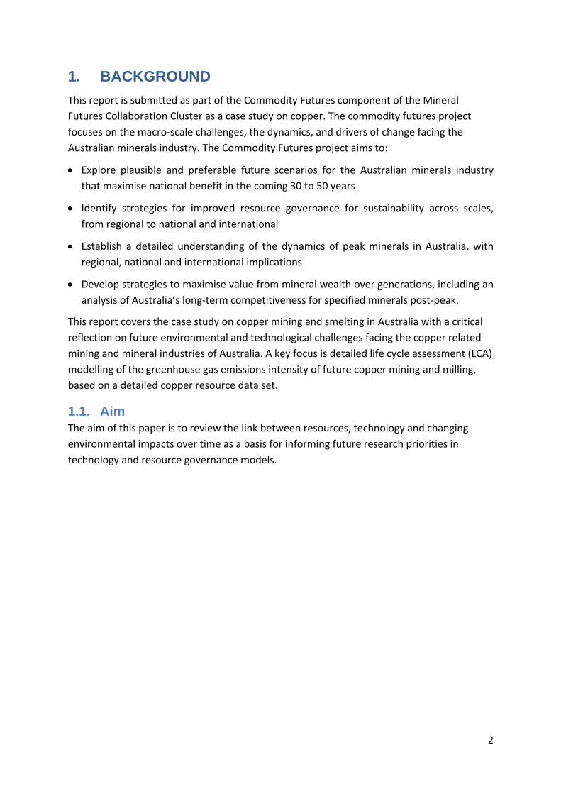
2.1. Global copper production World copper production has been increasing at about 2.75% a year for over a hundred
years, as shown in Figure 1, including by country in recent decades. Over the past century,
the status of dominant copper producer has shifted from the USA to Chile, with moderate
production from a range of countries such as Australia, Canada and across southern Africa
and Europe, amongst others. Cumulative global copper production from 1770 to 2011 has
been approximately 596 Mt Cu.
An assessment of global copper resources was given by Memary et al. (2012), based on a
detailed compilation of individual project mineral resources as reported by numerous
mining companies. Based on global resources data (from Memary et al., 2012, including
updates from Mudd et al., 2012), Chile remains the dominant country with 658.2 Mt Cu,
with important resources in numerous countries around the world, including the USA, Peru
and Australia with 170.1, 168.2 and 126.9 Mt Cu, respectively. World copper resources were
at least 1,860 Mt Cu (including China).
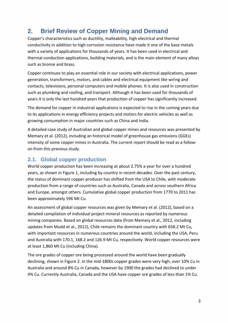
The ore grades of copper ore being processed around the world have been gradually
declining, shown in Figure 2. In the mid‐1800s copper grades were very high, over 10% Cu in
Australia and around 8% Cu in Canada, however by 1900 the grades had declined to under
4% Cu. Currently Australia, Canada and the USA have copper ore grades of less than 1% Cu.
4
Figure 1: World copper production (ex‐mine) by selected countries and region, 1880 to 2011, with inset of fractional production (data from Mudd et al, 2012).
Figure 2: Copper ore grade over time in select countries (Mudd et al., 2012).
0
2
4
6
8
10
12
14
16
1880
1890
1900
1910
1920
1930
1940
1950
1960
1970
1980
1990
2000
2010
An
nu
al C
op
per
Pro
du
ctio
n (
Mt
Cu
)
USA
AustraliaCanada
Chile
China
Africa
Europe
Restof theWorld
0
0.1
0.2
0.3
0.4
0.5
0.6
0.7
0.8
0.9
1
188
0
189
0
190
0
191
0
192
0
193
0
194
0
195
0
196
0
197
0
198
0
199
0
200
0
201
0
An
nu
al
Co
pp
er P
rod
uc
tio
n (
%p
rop
ort
ion
)
USA
Australia
Canada Chile
China
Africa
Europe
Restof theWorld
0
1
2
3
4
5
6
7
1900 1910 1920 1930 1940 1950 1960 1970 1980 1990 2000 2010
Co
pp
er O
re G
rad
e (
Cu
/%)
USA
Canada
World
Australia
Papua New Guinea
India
0
3
6
9
12
15
18
21
24
27
1840 1860 1880 1900 1920 1940 1960 1980 2000
Co
pp
er
Ore
Gra
de
(C
u/%
)
5
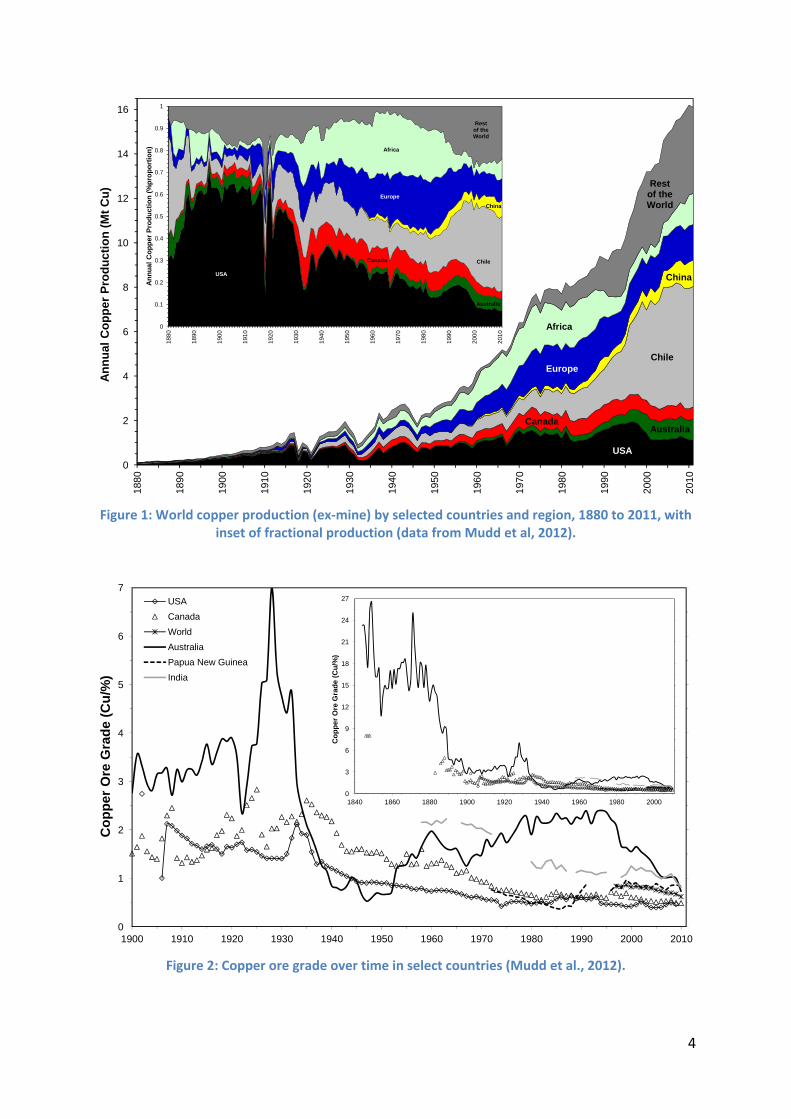
The nominal and real price of copper over time is shown in Figure 3, showing that the real
price has generally declined since 1900, even allowing for boom‐bust price cycles. The
factors influencing the world average copper price are many, and can include energy
(especially diesel and electricity), water, transport, demand / supply balance, mining and ore
processing technology, labour, mine waste management, government and industry policy,
new (or declining) uses, scale and rate of industrial and urban development (eg. China,
India, Africa, etc.), and so on.
Figure 3: The price of copper over time (data from Kelly & Matos, 2012).
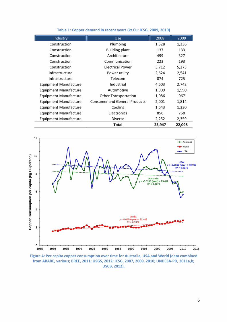
2.2. Copper demand The breakdown of copper uses is shown in Table 1. There is a strong demand for copper as it
is used in electrical applications, power generation, transformers, motors, and cables and
electronic devices. It is also used in construction such as plumbing and roofing, and
transport. Copper is an important resource in the electronics and construction industries.
In general, copper consumption is closely linked to per capita GDP, with more developed
countries having a higher consumption rate than less developed countries. Trends in per
capita copper consumption in recent decades are shown in Figure 4 for the USA, Australia
and the world. For the USA and Australia, per capita copper consumption was relatively
stable throughout the latter half of the twentieth century, averaging between 6 to 10 kg
Cu/person/year, but has declined steadily over the 2000s (now ~6 kg Cu/person/year). In
contrast, world per capita copper consumption has been gradually rising over the past fifty
years from ~1.6 to ~2.8 kg Cu/person/year.
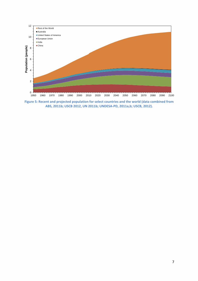
In global terms, per capita consumption is expected to continue to increase, given the
ongoing industrialisation and urbanisation of China and India (with other regions such as
Africa, South‐East Asia and South America also likely to emerge in coming decades as major
development hubs) as well as ongoing population growth (shown in Figure 5).
0.0
0.2
0.4
0.6
0.8
1.0
1.2
1.4
0
1,100
2,200
3,300
4,400
5,500
6,600
7,700
1900 1910 1920 1930 1940 1950 1960 1970 1980 1990 2000 2010
Ind
ex
ed
Re
al P
ric
e in
19
98
$ (
190
0 =
1)
No
min
al
Pri
ce
(US
$/t
Cu
)
Nominal Price
IndexedReal Price
6
Table 1: Copper demand in recent years (kt Cu; ICSG, 2009, 2010)
Industry Use 2008 2009
Construction Plumbing 1,528 1,336
Construction Building plant 137 133
Construction Architecture 499 327
Construction Communication 223 193
Construction Electrical Power 3,712 5,273
Infrastructure Power utility 2,624 2,541
Infrastructure Telecom 874 725
Equipment Manufacture Industrial 4,603 2,742
Equipment Manufacture Automotive 1,909 1,590
Equipment Manufacture Other Transportation 1,086 967
Equipment Manufacture Consumer and General Products 2,001 1,814
Equipment Manufacture Cooling 1,643 1,330
Equipment Manufacture Electronics 856 768
Equipment Manufacture Diverse 2,252 2,359
Total 23,947 22,098
Figure 4: Per capita copper consumption over time for Australia, USA and World (data combined from ABARE, various; BREE, 2011; USGS, 2012; ICSG, 2007, 2009, 2010; UNDESA‐PD, 2011a,b;
USCB, 2012).
Australia:y = -0.0108 (year) + 29.412
R² = 0.0278
World:y = 0.0169 (year) - 31.488
R² = 0.7482
USA:y = -0.0163 (year) + 40.903
R² = 0.0371
0
2
4
6
8
10
12
1955 1960 1965 1970 1975 1980 1985 1990 1995 2000 2005 2010 2015
Co
pp
er
Co
nsu
mp
tio
n p
er c
ap
ita
(kg
Cu
/pe
rso
n)
Australia
World
USA
7
Figure 5: Recent and projected population for select countries and the world (data combined from ABS, 2011b; USCB 2012, UN 2011b; UNDESA‐PD, 2011a,b; USCB, 2012).
0
2
4
6
8
10
12
1950 1960 1970 1980 1990 2000 2010 2020 2030 2040 2050 2060 2070 2080 2090 2100
Po
pu
lati
on
(p
eop
le)
Rest of the World
Australia
United States of America
European Union
India
China
8
3. Climate Change Impacts of Copper Mining
3.1. Life cycle assessment of copper production Life Cycle Assessment (LCA) is defined as the “compilation and evaluation of the inputs,
outputs and the potential environmental impacts of a product system throughout its life
cycle” (ISO, 2006). Many studies have used LCA to show the footprint of different
commodities including copper (see Norgate & Rankin, 2000; Norgate et al., 2004, 2007;
Fthenakis et al., 2009). The LCA guideline of Leiden University is used in this study (Guinée
et al., 2001). LCA has four main stages including goal and scope definition; inventory
analysis; impact assessment; and interpretation (ISO, 2006).
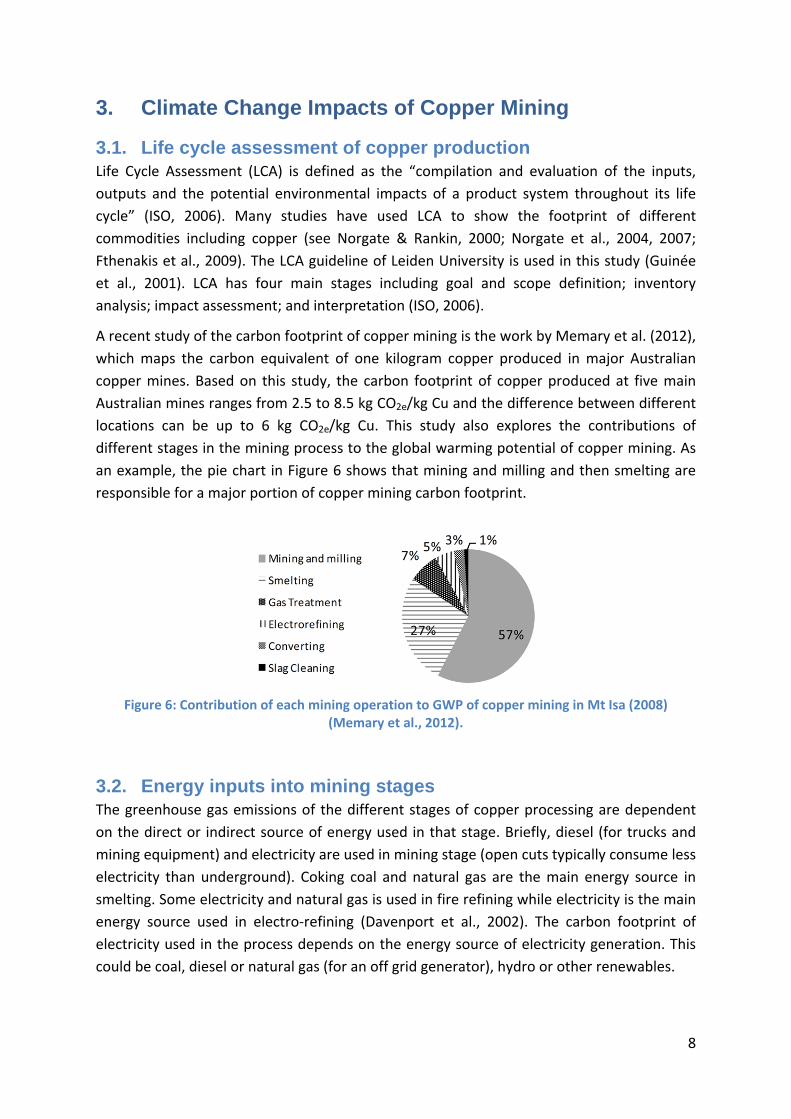
A recent study of the carbon footprint of copper mining is the work by Memary et al. (2012),
which maps the carbon equivalent of one kilogram copper produced in major Australian
copper mines. Based on this study, the carbon footprint of copper produced at five main
Australian mines ranges from 2.5 to 8.5 kg CO2e/kg Cu and the difference between different
locations can be up to 6 kg CO2e/kg Cu. This study also explores the contributions of
different stages in the mining process to the global warming potential of copper mining. As
an example, the pie chart in Figure 6 shows that mining and milling and then smelting are
responsible for a major portion of copper mining carbon footprint.
Figure 6: Contribution of each mining operation to GWP of copper mining in Mt Isa (2008) (Memary et al., 2012).
3.2. Energy inputs into mining stages The greenhouse gas emissions of the different stages of copper processing are dependent
on the direct or indirect source of energy used in that stage. Briefly, diesel (for trucks and
mining equipment) and electricity are used in mining stage (open cuts typically consume less
electricity than underground). Coking coal and natural gas are the main energy source in
smelting. Some electricity and natural gas is used in fire refining while electricity is the main
energy source used in electro‐refining (Davenport et al., 2002). The carbon footprint of
electricity used in the process depends on the energy source of electricity generation. This
could be coal, diesel or natural gas (for an off grid generator), hydro or other renewables.
9
3.3. Relationship between ore grade and carbon intensity of final product
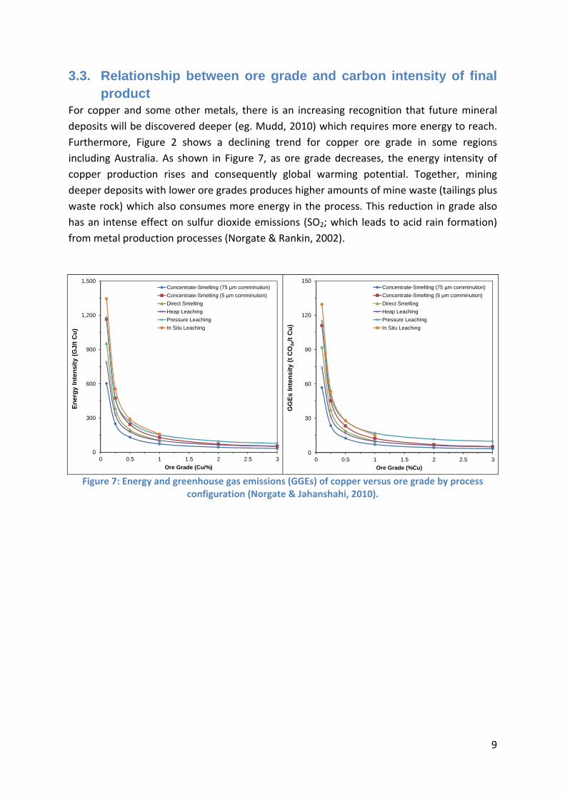
For copper and some other metals, there is an increasing recognition that future mineral
deposits will be discovered deeper (eg. Mudd, 2010) which requires more energy to reach.
Furthermore, Figure 2 shows a declining trend for copper ore grade in some regions
including Australia. As shown in Figure 7, as ore grade decreases, the energy intensity of
copper production rises and consequently global warming potential. Together, mining
deeper deposits with lower ore grades produces higher amounts of mine waste (tailings plus
waste rock) which also consumes more energy in the process. This reduction in grade also
has an intense effect on sulfur dioxide emissions (SO2; which leads to acid rain formation)
from metal production processes (Norgate & Rankin, 2002).
Figure 7: Energy and greenhouse gas emissions (GGEs) of copper versus ore grade by process configuration (Norgate & Jahanshahi, 2010).
0
300
600
900
1,200
1,500
0 0.5 1 1.5 2 2.5 3
En
erg
y In
ten
sity
(G
J/t
Cu
)
Ore Grade (Cu/%)
Concentrate-Smelting (75 µm comminution)
Concentrate-Smelting (5 µm comminution)
Direct Smelting
Heap Leaching
Pressure Leaching
In Situ Leaching
0
30
60
90
120
150
0 0.5 1 1.5 2 2.5 3
GG
Es
Inte
ns
ity
(t C
O2e
/t C
u)
Ore Grade (%Cu)
Concentrate-Smelting (75 µm comminution)
Concentrate-Smelting (5 µm comminution)
Direct Smelting
Heap Leaching
Pressure Leaching
In Situ Leaching
10
4. Methodology
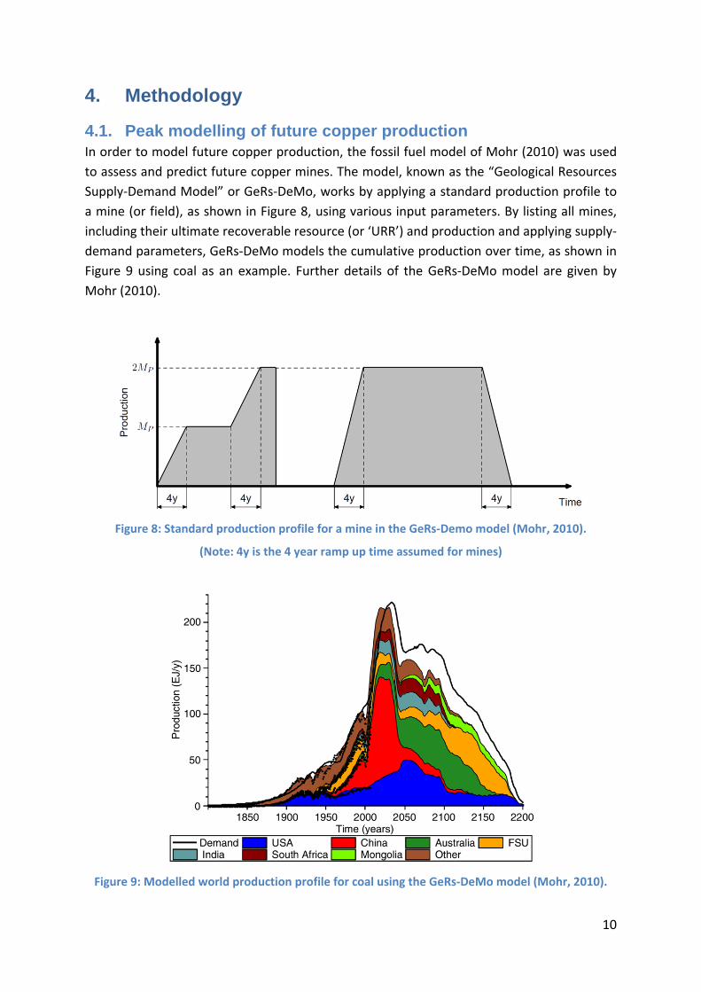
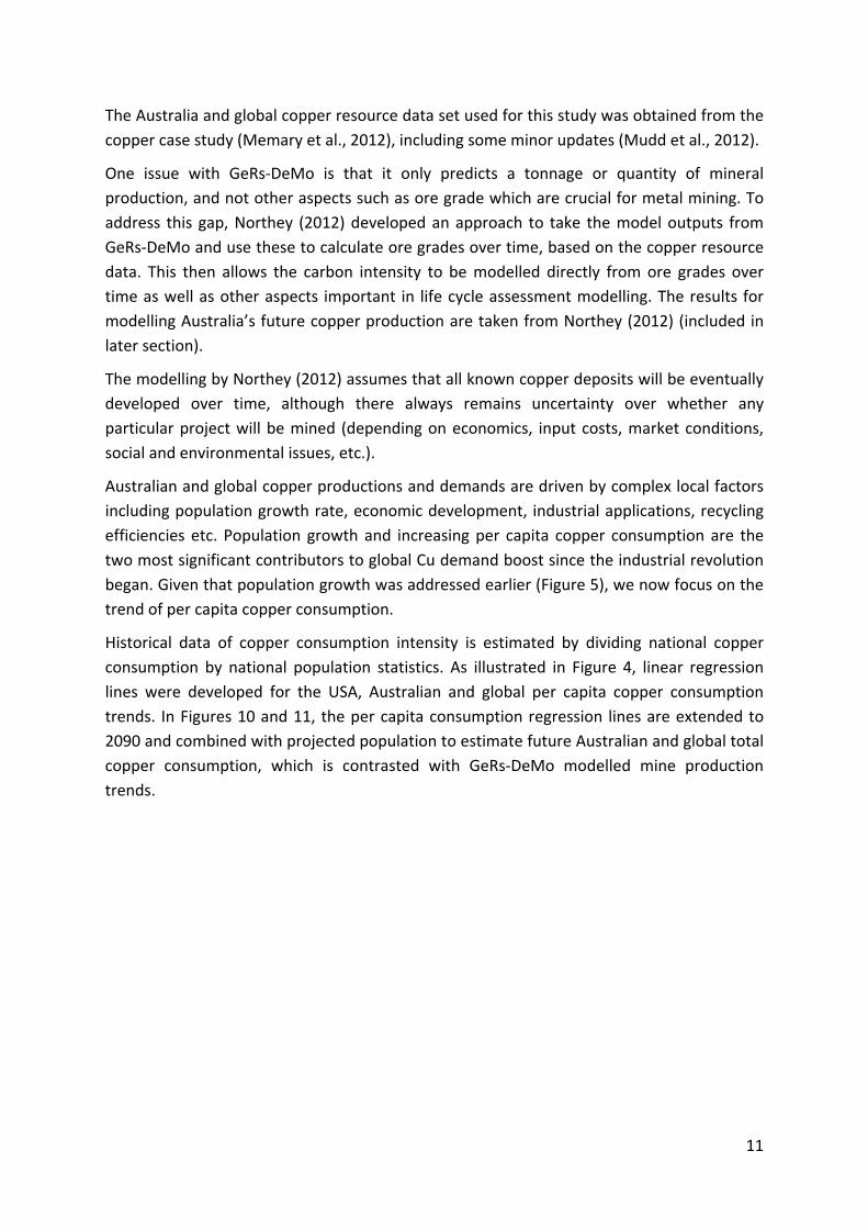
4.1. Peak modelling of future copper production In order to model future copper production, the fossil fuel model of Mohr (2010) was used
to assess and predict future copper mines. The model, known as the “Geological Resources
Supply‐Demand Model” or GeRs‐DeMo, works by applying a standard production profile to
a mine (or field), as shown in Figure 8, using various input parameters. By listing all mines,
including their ultimate recoverable resource (or ‘URR’) and production and applying supply‐
demand parameters, GeRs‐DeMo models the cumulative production over time, as shown in
Figure 9 using coal as an example. Further details of the GeRs‐DeMo model are given by
Mohr (2010).
Figure 8: Standard production profile for a mine in the GeRs‐Demo model (Mohr, 2010).
(Note: 4y is the 4 year ramp up time assumed for mines)
Figure 9: Modelled world production profile for coal using the GeRs‐DeMo model (Mohr, 2010).
11
The Australia and global copper resource data set used for this study was obtained from the
copper case study (Memary et al., 2012), including some minor updates (Mudd et al., 2012).
One issue with GeRs‐DeMo is that it only predicts a tonnage or quantity of mineral
production, and not other aspects such as ore grade which are crucial for metal mining. To
address this gap, Northey (2012) developed an approach to take the model outputs from
GeRs‐DeMo and use these to calculate ore grades over time, based on the copper resource
data. This then allows the carbon intensity to be modelled directly from ore grades over
time as well as other aspects important in life cycle assessment modelling. The results for
modelling Australia’s future copper production are taken from Northey (2012) (included in
later section).
The modelling by Northey (2012) assumes that all known copper deposits will be eventually
developed over time, although there always remains uncertainty over whether any
particular project will be mined (depending on economics, input costs, market conditions,
social and environmental issues, etc.).
Australian and global copper productions and demands are driven by complex local factors
including population growth rate, economic development, industrial applications, recycling
efficiencies etc. Population growth and increasing per capita copper consumption are the
two most significant contributors to global Cu demand boost since the industrial revolution
began. Given that population growth was addressed earlier (Figure 5), we now focus on the
trend of per capita copper consumption.
Historical data of copper consumption intensity is estimated by dividing national copper
consumption by national population statistics. As illustrated in Figure 4, linear regression
lines were developed for the USA, Australian and global per capita copper consumption
trends. In Figures 10 and 11, the per capita consumption regression lines are extended to
2090 and combined with projected population to estimate future Australian and global total
copper consumption, which is contrasted with GeRs‐DeMo modelled mine production
trends.

12
Figure 10: Projected global copper demand and mine production to 2090.
Figure 11: Projected Australian copper demand and mine production to 2090.
Figure 10 shows global copper demand could be readily satisfied by mine production until
the early 2040s, with a peak annual global production rate of 27.7 Mt Cu in 2044. Beyond
this time, increasing global demand cannot be met by mine production alone. In other
words, more emphasis on copper recycling and improving efficiency is not only a choice but
rather a necessity on a global scale.
Projections of Australian copper demand and mine production over the next century (Figure
11) show that Australia will produce far in excess of demand until 2070, when all deposits
are effectively exhausted. Until this time, this allows Australia to continue to be a major
copper exporter.
0
9
18
27
36
45
2010 2020 2030 2040 2050 2060 2070 2080 2090
Pro
du
cto
n v
s D
em
and
(M
t C
u/Y
ear
)Global Demand
Global Production
0
0.4
0.8
1.2
1.6
2
2.4
2010 2020 2030 2040 2050 2060 2070 2080 2090
Pro
du
cto
n v
s D
em
and
(M
t C
u/Y
ear
)
Australian Demand
Australian Production
13
4.2. LCA model of copper mining All Australian copper projects (from Memary et al., 2012) were classified based on mine
type and processing configuration for existing mines, while assumptions were made about
deposits concerning their likely development (eg. open cut or underground, flotation or
heap leach with solvent extraction‐electrowinning). The main configurations are thus:
Open cut and flotation – producing a copper concentrate;
Underground and flotation – producing a copper concentrate;
Open cut and heap leach‐solvent extraction‐electrowinning – producing refined copper
metal;
Underground and heap leach‐solvent extraction‐electrowinning – producing refined
copper metal;
Miscellaneous – mixed open cut and underground mine with flotation, mixed open cut
and underground mine with heap leach, or underground mine and heap leach.
The full list of Australian copper deposits and their mine and process configuration is
provided in Appendix 1.
In this way, the LCA model for copper mining by Giurco (2005) can be applied based on the
primary stages involved in copper production. This model was also used to model historical
copper mining in Australia by Memary et al. (2012). Although the Giurco model includes all
four primary stages of mining, milling, smelting and refining, this study will only analyse
mining and milling since the vast majority of projects (existing and future) do not include a
smelter at the project site. The only existing copper smelters (Mt Isa and Olympic Dam) and
refineries (Olympic Dam and Townsville) in Australia are very unlikely to be expanded based
on current cost pressures in the industry, with the Mt Isa and Townsville facilities currently
scheduled by owner Xstrata to be closed in 2016 and the proposed Olympic Dam expansion
recently postponed indefinitely by BHP Billiton. Hence all existing and future copper projects
in Australia will be essentially mining and milling only (except for heap leach projects, which,
based on deposit types and assumed configurations, appear likely to be minor in scale and
production compared to flotation‐based projects).
There were two primary approaches to LCA modelling of future Australian copper
production:
1. State / Local Grid Model – all mines were grouped based on their respective electricity
grid (or source), to allow for a specific carbon intensity for electricity. Although most
states only have a single electricity grid, states such as Queensland and Western Australia
have numerous mines in remote areas not connected to the main state grid. An LCA
model was then developed for each grid‐based group and project configuration. For
example, all copper projects around Mt Isa were grouped since they are connected to the
gas‐fired electricity grid for Mt Isa, while projects in eastern Queensland were assumed
to be connected to the black coal‐based electrical grid.
14
2. Australian Model – Based on the copper produced from all projects of a given
configuration, such as open cut‐flotation or underground flotation. A separate LCA model
was developed for each configuration, using the modelled copper production from
Northey (2012) and calculated ore grade from the projects involved in this configuration.
Four LCA models were run separately and then combined to give the Australian total.
3. Global Model – Based on the global copper production model by Northey (2012), a basic
global LCA model was developed assuming a constant ratio of 85%‐15% by open cut‐
underground (Scenario 1), or starting at 85%‐15% and moving to 50%‐50% by 2100
(Scenario 2), respectively. It was assumed that all projects used flotation.
The dominant energy inputs to copper mining and milling are electricity and diesel, leading
to significant greenhouse gas emissions per tonne of copper (ie. carbon intensity). In order
to assess the effectiveness of low carbon energy inputs to decrease the carbon intensity,
different energy scenarios were modelled, specifically:
1. Grid‐based Electricity – electricity sourced from the local grid, either state main grid or
separate regional grid, transportation is assumed to be petroleum‐derived diesel. This is
a “business‐as‐usual” scenario.
2. Natural Gas‐based Electricity – all electricity sourced from natural gas. This is a “partial
transition” scenario.
3. Solar Thermal Electricity – assuming that electricity was obtained from baseload solar
thermal power plants, with a carbon intensity of 0.05 kg CO2e/kWh (see Lenzen, 2010).
This represents a more “comprehensive transition” scenario.
4. Solar Thermal Electricity and Biodiesel Transport Fuel – all diesel consumed in mine
vehicles comes from biodiesel, with a carbon intensity of 10.63 kg CO2e/t diesel; based on
biodiesel being a renewable fuel, with the carbon released being absorbed in re‐growing
the source oil feedstock (as defined by climate change carbon accounting conventions;
see DCCEE, 2011). All electricity consumed in mining process are assumed to be satisfied
by solar power network. This represents a “very optimistic transition” scenario.
Details of emission factors implemented are summarised in Table 2.
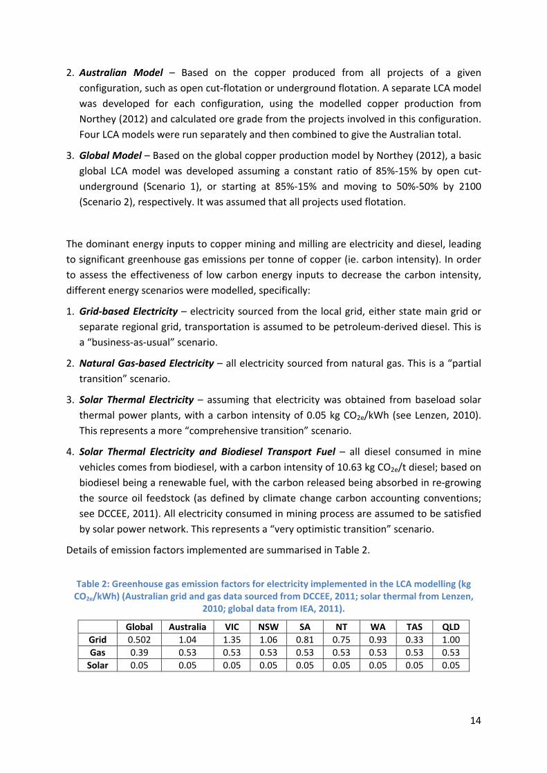
Table 2: Greenhouse gas emission factors for electricity implemented in the LCA modelling (kg CO2e/kWh) (Australian grid and gas data sourced from DCCEE, 2011; solar thermal from Lenzen,
2010; global data from IEA, 2011).
Global Australia VIC NSW SA NT WA TAS QLD
Grid 0.502 1.04 1.35 1.06 0.81 0.75 0.93 0.33 1.00
Gas 0.39 0.53 0.53 0.53 0.53 0.53 0.53 0.53 0.53
Solar 0.05 0.05 0.05 0.05 0.05 0.05 0.05 0.05 0.05
15
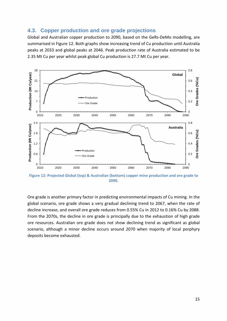
4.3. Copper production and ore grade projections Global and Australian copper production to 2090, based on the GeRs‐DeMo modelling, are
summarised in Figure 12. Both graphs show increasing trend of Cu production until Australia
peaks at 2033 and global peaks at 2046. Peak production rate of Australia estimated to be
2.35 Mt Cu per year whilst peak global Cu production is 27.7 Mt Cu per year.
Figure 12: Projected Global (top) & Australian (bottom) copper mine production and ore grade to 2090.
Ore grade is another primary factor in predicting environmental impacts of Cu mining. In the
global scenario, ore grade shows a very gradual declining trend to 2067, when the rate of
decline increase, and overall ore grade reduces from 0.55% Cu in 2012 to 0.16% Cu by 2088.
From the 2070s, the decline in ore grade is principally due to the exhaustion of high grade
ore resources. Australian ore grade does not show declining trend as significant as global
scenario, although a minor decline occurs around 2070 when majority of local porphyry
deposits become exhausted.
0
0.2
0.4
0.6
0.8
0
7
14
21
28
2010 2020 2030 2040 2050 2060 2070 2080 2090
Ore
Gra
des
(%
Cu
)
Pro
du
ctio
n (
Mt
Cu
/yea
r)
Production
Ore Grade
Global
0
0.2
0.4
0.6
0.8
0
0.6
1.2
1.8
2.4
2010 2020 2030 2040 2050 2060 2070 2080 2090
Ore
Gra
des
(%
Cu
)
Pro
du
ctio
n (
Mt
Cu
/yea
r)
Production
Ore Grade
Australia
16
5. Results
5.1. Greenhouse gas emissions projections of global copper mining
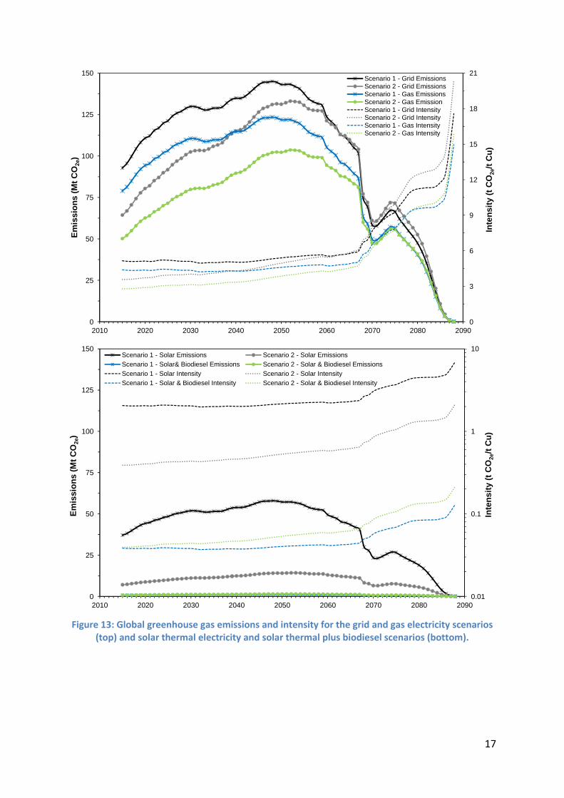
There are two scenarios of Global Copper production which were implemented in LCA
modelling. Scenario 1 assumes constant 85% open cut and 15% underground mining
configurations of all copper mines (based on production data in Mudd & Weng, 2012);
Scenario 2 initially assumes the ratio of 85% open cut and 15% underground mining and
moving to 50‐50% open cut and underground mining by 2100. By combining each
production scenario with emissions factors from Table 2, results of global copper mining
emissions are plotted in Figure 13.
Generally, due to higher percentages of open cut mining in Scenario 1, its emission rate and
intensity is almost always higher than Scenario 2 in the three electricity source (Grid, Gas
and Solar) models. The only exception is the ‘Solar Thermal Electricity and Biodiesel
Transport Fuel’ model in which Scenario 2 has slightly higher emission rate and intensity.
Overall trends of total greenhouse gas emissions from Cu mining are driven mainly by
annual Cu production while the pollution intensities are closely related to ore grade (as
expected). As shown from Figures 12 and 13, when global ore grade begins to rapidly
decline from the late 2060s, the greenhouse gas emissions intensity of Cu mining also
increases significantly.
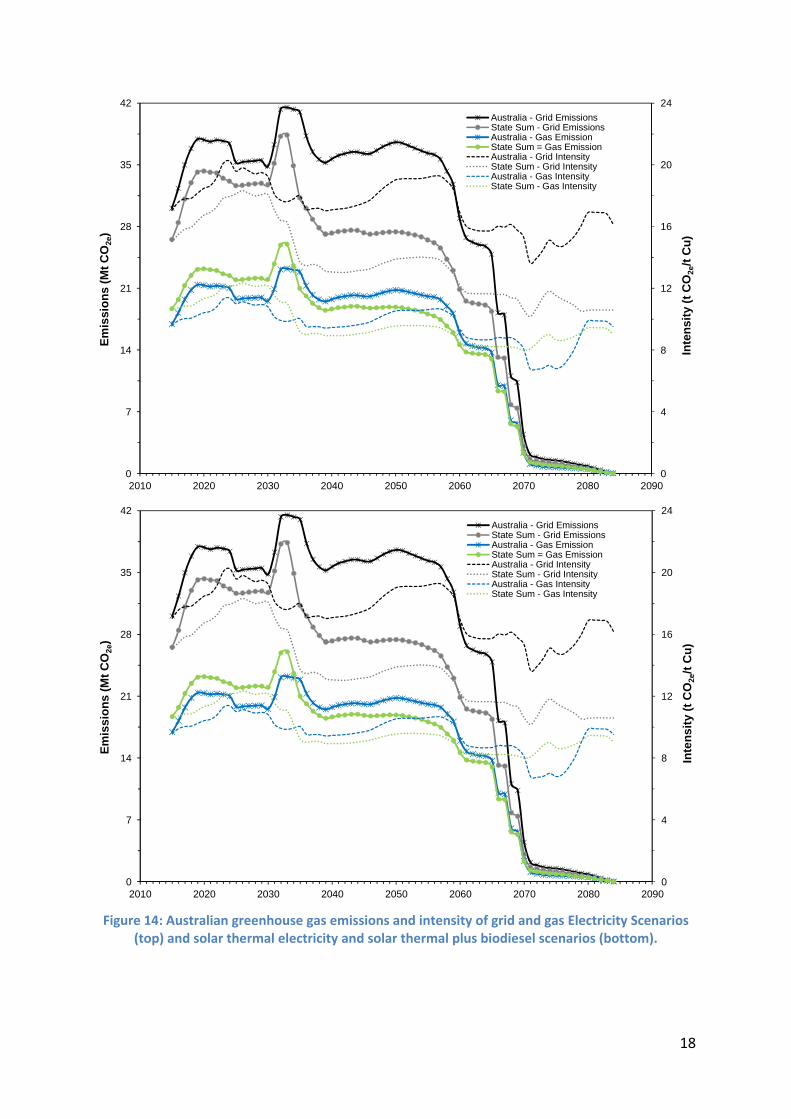
5.2. Greenhouse gas emissions projections of Australian copper mining
For the Australian models, all Victorian (VIC), Tasmanian (TAS) and New South Wales (NSW)
projects are connected to the state grid for LCA modelling purposes, using the respective
state average grid emissions factors. The Mt Isa region is dependent on natural gas‐fired
power station. Where a project not connected to the state grid is using natural gas for
electricity, we allocated it to the “Mt Isa Group”. While some West Australian (WA) projects
are reliant on electricity from diesel‐based generators, the emissions intensity for such
electricity is virtually identical to the WA state grid factor, and hence such projects were
included in the “WA grid model”. Full details of the classification of all mines and projects
are provided in Appendix 1. Deposits with complex open cut and underground
configurations are assumed to have a production ratio between open cut and underground
of 50‐50%. As such, the “State Sum” model is the summary of all individual state and
regional based models while the “Australia” model is based on national average emissions
factor and Cu production rates. All modelling results are plotted in Figure 14.
17
Figure 13: Global greenhouse gas emissions and intensity for the grid and gas electricity scenarios (top) and solar thermal electricity and solar thermal plus biodiesel scenarios (bottom).
0
3
6
9
12
15
18
21
0
25
50
75
100
125
150
2010 2020 2030 2040 2050 2060 2070 2080 2090
Inte
nsi
ty (
t C
O2e
/t C
u)
Em
issi
on
s (
Mt
CO
2e)
Scenario 1 - Grid EmissionsScenario 2 - Grid EmissionsScenario 1 - Gas EmissionsScenario 2 - Gas EmissionScenario 1 - Grid IntensityScenario 2 - Grid IntensityScenario 1 - Gas IntensityScenario 2 - Gas Intensity
0.01
0.1
1
10
0
25
50
75
100
125
150
2010 2020 2030 2040 2050 2060 2070 2080 2090
Inte
ns
ity
(t C
O2e
/t C
u)
Em
issi
on
s (
Mt
CO
2e)
Scenario 1 - Solar Emissions Scenario 2 - Solar Emissions
Scenario 1 - Solar& Biodiesel Emissions Scenario 2 - Solar & Biodiesel Emissions
Scenario 1 - Solar Intensity Scenario 2 - Solar Intensity
Scenario 1 - Solar & Biodiesel Intensity Scenario 2 - Solar & Biodiesel Intensity
18
Figure 14: Australian greenhouse gas emissions and intensity of grid and gas Electricity Scenarios (top) and solar thermal electricity and solar thermal plus biodiesel scenarios (bottom).
0
4
8
12
16
20
24
0
7
14
21
28
35
42
2010 2020 2030 2040 2050 2060 2070 2080 2090
Inte
nsi
ty (
t C
O2e
/t C
u)
Em
issi
on
s (M
t C
O2e
)Australia - Grid EmissionsState Sum - Grid EmissionsAustralia - Gas EmissionState Sum = Gas EmissionAustralia - Grid IntensityState Sum - Grid IntensityAustralia - Gas IntensityState Sum - Gas Intensity
0
4
8
12
16
20
24
0
7
14
21
28
35
42
2010 2020 2030 2040 2050 2060 2070 2080 2090
Inte
nsi
ty (
t C
O2e
/t C
u)
Em
issi
on
s (
Mt
CO
2e)
Australia - Grid EmissionsState Sum - Grid EmissionsAustralia - Gas EmissionState Sum = Gas EmissionAustralia - Grid IntensityState Sum - Grid IntensityAustralia - Gas IntensityState Sum - Gas Intensity
19
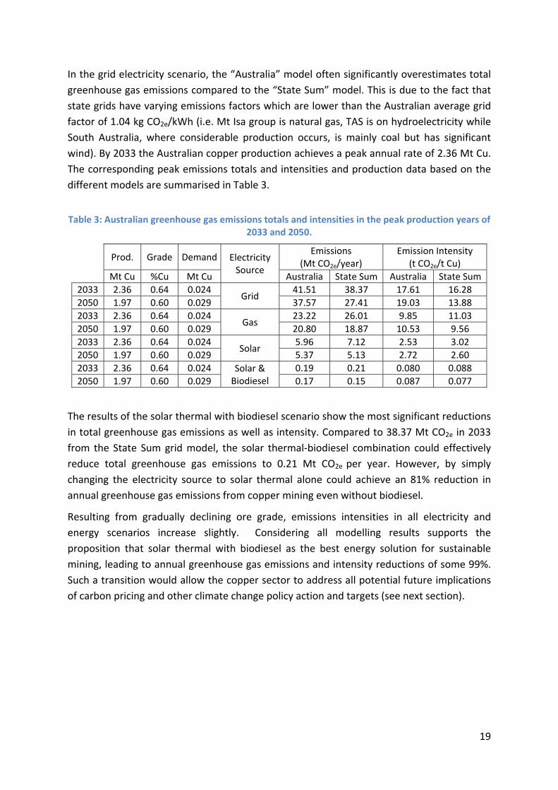
In the grid electricity scenario, the “Australia” model often significantly overestimates total
greenhouse gas emissions compared to the “State Sum” model. This is due to the fact that
state grids have varying emissions factors which are lower than the Australian average grid
factor of 1.04 kg CO2e/kWh (i.e. Mt Isa group is natural gas, TAS is on hydroelectricity while
South Australia, where considerable production occurs, is mainly coal but has significant
wind). By 2033 the Australian copper production achieves a peak annual rate of 2.36 Mt Cu.
The corresponding peak emissions totals and intensities and production data based on the
different models are summarised in Table 3.
Table 3: Australian greenhouse gas emissions totals and intensities in the peak production years of
2033 and 2050.
Prod. Grade Demand Electricity Source
Emissions (Mt CO2e/year)
Emission Intensity (t CO2e/t Cu)
Mt Cu %Cu Mt Cu Australia State Sum Australia State Sum
2033 2.36 0.64 0.024 Grid
41.51 38.37 17.61 16.28
2050 1.97 0.60 0.029 37.57 27.41 19.03 13.88
2033 2.36 0.64 0.024 Gas
23.22 26.01 9.85 11.03
2050 1.97 0.60 0.029 20.80 18.87 10.53 9.56
2033 2.36 0.64 0.024 Solar
5.96 7.12 2.53 3.02
2050 1.97 0.60 0.029 5.37 5.13 2.72 2.60
2033 2.36 0.64 0.024 Solar & Biodiesel
0.19 0.21 0.080 0.088
2050 1.97 0.60 0.029 0.17 0.15 0.087 0.077
The results of the solar thermal with biodiesel scenario show the most significant reductions
in total greenhouse gas emissions as well as intensity. Compared to 38.37 Mt CO2e in 2033
from the State Sum grid model, the solar thermal‐biodiesel combination could effectively
reduce total greenhouse gas emissions to 0.21 Mt CO2e per year. However, by simply
changing the electricity source to solar thermal alone could achieve an 81% reduction in
annual greenhouse gas emissions from copper mining even without biodiesel.
Resulting from gradually declining ore grade, emissions intensities in all electricity and
energy scenarios increase slightly. Considering all modelling results supports the
proposition that solar thermal with biodiesel as the best energy solution for sustainable
mining, leading to annual greenhouse gas emissions and intensity reductions of some 99%.
Such a transition would allow the copper sector to address all potential future implications
of carbon pricing and other climate change policy action and targets (see next section).
20
6. Analysis & Discussion
The mining and use of copper is inextricably linked to technology in a variety of ways – from
exploration, mining and refining through manufacture to use and possible recycling. This
study has focussed on modelling the mining and milling stages of copper production,
especially the greenhouse gas emissions intensity, using a variety of energy and electricity
scenarios. This section presents a brief discussion and analysis of the findings and their
implications for copper mining in Australia, as well mining more generally, especially with
respect to long‐term greenhouse gas emissions targets.
6.1. Greenhouse gas emissions targets and trajectories The medium and long‐term targets for reductions in total greenhouse gas emissions for
Australia are (DCCEE, 2012):
5% from 2000 levels by 2020 without any global commitments;
15% from 2000 levels by 2020 if global commitments seek to achieve stabilisation of
atmospheric CO2e levels of between 510 to 540 ppm;
25% from 2000 levels by 2020 if global commitments seek to achieve stabilisation of
atmospheric CO2e levels of 450 ppm;
80% from 2000 levels by 2050 as an aspirational goal.
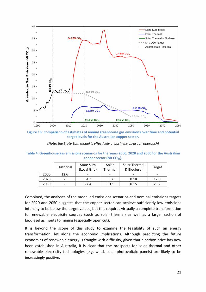
Australia’s total greenhouse gas emissions in 2000 were 558 Mt CO2e (DCCEE, 2010),
although there is no breakdown of emissions inventory data whereby copper mining is
separated out for its reported emissions. As such, approximate emissions from 1990 to 2010
are calculated based on a nominal value of 15 t CO2e/t Cu and national copper production.
For the year 2000, where production was 839,000 t Cu, this gives estimated emissions of
12.6 Mt CO2e. The medium and long‐term emissions targets are then estimated from this
value and compared to the electricity and energy scenarios presented previously, using the
state sum model, and this is shown in Figure 15 and summarised in Table 4. It is assumed
that all emissions reductions are shared equally across the economy.
From this graph, it is clear that adoption of solar thermal technology as the dominant
electricity source allows substantial emissions reductions to be achieved and this would
ensure that the copper sector is well below the nominal target of 12.0 Mt CO2e. By 2050,
however, the target becomes 2.52 Mt CO2e and the solar thermal only scenario projects
emissions of 5.13 Mt CO2e – still above the 2050 goal. The solar thermal plus biodiesel
scenario projects emissions of 0.15 Mt CO2e – significantly below the 2050 goal. Another
alternative approach, not modelled in this study, is to electrify mining vehicle fleets and
provide the electricity via solar thermal plants also. Given the increased energy efficiency of
such an approach (i.e. high conversion of the embodied electricity into application), this
could present even further opportunities for reducing energy inputs and reducing the
environmental footprint of copper production.
21
Figure 15: Comparison of estimates of annual greenhouse gas emissions over time and potential target levels for the Australian copper sector.
(Note: the State Sum model is effectively a ‘business‐as‐usual’ approach)
Table 4: Greenhouse gas emissions scenarios for the years 2000, 2020 and 2050 for the Australian
copper sector (Mt CO2e).
Historical State Sum (Local Grid)
Solar Thermal
Solar Thermal & Biodiesel
Target
2000 12.6 ‐ ‐ ‐ ‐
2020 ‐ 34.3 6.62 0.18 12.0
2050 ‐ 27.4 5.13 0.15 2.52
Combined, the analyses of the modelled emissions scenarios and nominal emissions targets
for 2020 and 2050 suggests that the copper sector can achieve sufficiently low emissions
intensity to be below the target values, but this requires virtually a complete transformation
to renewable electricity sources (such as solar thermal) as well as a large fraction of
biodiesel as inputs to mining (especially open cut).
It is beyond the scope of this study to examine the feasibility of such an energy
transformation, let alone the economic implications. Although predicting the future
economics of renewable energy is fraught with difficulty, given that a carbon price has now
been established in Australia, it is clear that the prospects for solar thermal and other
renewable electricity technologies (e.g. wind, solar photovoltaic panels) are likely to be
increasingly positive.
0
5
10
15
20
25
30
35
40
1990 2000 2010 2020 2030 2040 2050 2060 2070 2080
Gre
enh
ou
se G
as
Em
issi
on
s (
Mt
CO
2e)
State Sum Model
Solar Thermal
Solar Thermal + Biodiesel
Mt CO2e Target
Approximate Historical
34.3 Mt CO2e
27.4 Mt CO2e
6.62 Mt CO2e
5.13 Mt CO2e
12.0 Mt CO2e
12.6
Mt
CO
2e
2.52 Mt CO2e
0.18 Mt CO2e 0.15 Mt CO2e
22
A final point should be made that energy efficiency remains a crucial part of future mining,
and can be a very low cost manner in which to reduce the environmental footprint of mining
and metal production, as well as giving an important reduction in operating costs.
Overall, the ‘business‐as‐usual’ approach in the copper sector (i.e. the State Sum model) will
see it increasingly exposed to the price of carbon, mainly as production increases in
Australia with either brownfields expansions or new projects coming on‐stream. Based on
the scenarios modelled in this study, transformation of the copper sector to 100%
renewable energy sources for both electricity and liquid fuels (or even perhaps
electrification of mining vehicle fleets) would ensure that the sector can contribute to
Australian and global action on reducing greenhouse gas emissions and substantially
eliminate its exposure to a carbon price.
6.2. Implications for the future of copper
The long‐term future of the copper industry is difficult to project given the complexity of
uses and challenges it faces. There are two primary aspects to examine – production and
use, with this study focussed on production.
From a resource perspective, as shown by Memary et al. (2012) and Mudd et al. (2012),
there are abundant deposits of copper already identified worldwide to sustain and increase
production to meet likely demand scenarios for several decades. The primary challenges will
therefore be in how production occurs – the technology used and associated environmental
(and social) impacts.
At present, open cut mining is the dominant form of ore extraction, while underground
mining is used at some deeper and generally higher grade projects. Given the increasing
depth of projects, it can be expected that in coming decades there will be a higher
proportion of underground mining, though this will be dependent on diesel prices, other
mining costs and especially site‐specific geological conditions at each project. For example,
the Cadia East copper‐gold project was originally planned as an open cut mine but this was
converted to underground only when seeking environmental approvals. An unusual
example of underground mining is the giant El Teniente copper mine in Chile, with an
annual extraction rate of about 47 Mt ore/year – making it one of the largest underground
mining operations in the world. In reality, it is hard to predict the future trends in mine type,
except to say that open cut mining will remain dominant for at least a few decades with
underground like to gradually increase its proportion over time, perhaps becoming
dominant later this century.
The main technologies used for copper mining are grinding and flotation to produce a
copper concentrate (often with significant values of gold and silver) or heap leaching
combined with solvent extraction and electrowinning (‘SX‐EW’) to produce a refined copper
metal. Although grinding and flotation remains the most widely used technology, heap
23
leaching with SX‐EW has averaged about 19% of global copper mine production over the
past decade (USGS, various). Based on the global copper resource data, a modest increase in
the use of heap leaching with SX‐EW can be expected in the future, although grinding and
flotation can be expected to remain the dominant process flowsheet.
A major issue with respect to grinding is the average particle size of grinding. In general, a
finer average grind size allows for improved recovery, especially from more refractory ores.
As analysed by Norgate and Jahanshahi (2010), if the average particle size is reduced from
75 µm to 5 µm the energy and emissions intensity of copper production increases
substantially as ore grades decline below 1% Cu. A detailed survey of grind size at existing
projects is beyond the scope of this study, although it is recognised in the mining industry
that finer grind sizes will be increasingly required at existing and future copper projects. This
focusses attention on the need to ensure energy efficient grinding, and that any new
technology is assessed against the energy intensity of existing technologies.
An alternative production approach is the use of ‘in‐situ leaching’ (ISL), whereby a deposit
exists either in a permeable horizon and process solutions can be injected via groundwater
bores and the copper‐rich solution then simply pumped out and passed through SX‐EW. The
use of ISL appears to be restricted to a very few projects with suitable geologic conditions,
although as shown in Figure 7, ISL‐based copper production appears to be more energy and
emissions intensive than standard coarse grinding, flotation and smelting‐refining.
Overall, there is a strong need to ensure that existing and future technologies used in
copper mining and milling (as well as smelting and refining) are assessed against current
performance benchmarks for energy and greenhouse gas emissions intensity. That is, if a
new technology or process configuration is proposed, it should be more efficient than
existing process technology.
As shown in Figure 4, some developed countries like the USA and Australia display a
significant reduction in domestic copper consumption per capita. In general, this is due to a
few different reasons (Takashi, 2005; Edelstein, 2008):
1. copper smelters and refineries with heavy pollution intensity are shifting to low cost
developing countries such as Chile and China;
2. modest recovery in refined copper demands but remains in low recession level;
3. increasing ratio of imported refined copper.
A similar declining trend of per capita copper consumption has occurred in Japan since 1990
as the focus of the national economic shifted from heavy industry and manufacturing to a
more service‐based economy (Takashi, 2005). In contrast, developing countries such as
China and Chile will keep increasing in both total copper demand as well as per capita
copper consumption due to strong urbanisation and industrialisation (Takashi, 2005). By
2015, China is expected to achieve an annual copper demand of 8 Mt Cu and 6 to 7 kg Cu
per capita demand (Cheng and Weixuan, 2011).
24
For Australia, copper demand will remain very modest by world standards compared to
China, India, North America and Europe, although the decline of manufacturing is likely to
continued downwards pressure on Australian copper demand.
Overall, the proportion of copper demand met by recycling will most likely continue to be
modest until the latter half of this century – depending on relative costs and benefits. For
example, if recycled copper was produced using renewable energy, the environmental
footprint would be considerably lower than primary production. In the long‐term, there is a
clear need and basis for copper recycling, although such detailed research was beyond the
scope of this study.
7. Conclusion In this study, we focussed on analysing the likely future environmental footprint of primary
copper supply, rather than how to meet copper demand. We develop a peak copper
production model, based on a detailed copper resource data set, and combine this with a
comprehensive life cycle assessment model of copper mining and milling to predict
greenhouse gas emission rates and intensities of Australian and global copper production up
to 2100. By establishing a quantitative prediction of both copper production and
corresponding greenhouse gas emissions of Australian and global copper industry, we then
analysed the emissions intensity of various energy input scenarios, such as business‐as‐
usual, solar thermal electricity and solar thermal electricity with biodiesel.
The Australian Government has an aspirational goal long‐term greenhouse gas emissions of
an 80% reduction from the 2000 level by 2050. For the copper sector, this means moving
from about 12.6 Mt CO2e in 2000 to a goal of some 2.52 Mt CO2e in 2050 (assuming equal
emissions reductions across the economy). Based on the energy sources modelled, only the
solar thermal plus biodiesel scenario was capable of achieving this goal at about 0.15 Mt
CO2e, since the solar thermal alone scenario still includes normal petro‐diesel as a major
source of emissions.
Overall, it is clear that there are abundant resources which can meet expected long‐term
copper demands, the critical issue is more the environmental footprint of different copper
supplies and use rather than how much is available for mining. It is clear that the switch to
renewable energy can have a profound impact on the carbon intensity of copper supply and
a complete conversion to renewable energy will position the copper sector to meet existing
annual greenhouse gas emissions targets and goals.

25
8. References ABARE, various, Australian Commodity Statistics (Years 1995‐2010). Australian Bureau of
Agricultural and Resource Economics (ABARE), Canberra, ACT
ABS, 2008, S3105.0.65.001 ‐ Australian Historical Population Statistics, Australian Bureau of
Statistics (ABS), Canberra, ACT.
ABS, 2011a, 3101.0 Australian Demographic Statistics, Australian Bureau of Statistics (ABS),
Canberra, ACT.
ABS, 2011b, 3222.0 Population Projections, Australia 2006 to 2101, Australian Bureau of
Statistics (ABS), Canberra, ACT.
BREE, 2011, Resources and Energy Statistics 2011. Bureau of Resource & Energy Economics
(BREE), Canberra, ACT, 174 p.
Cheng, M & Weixuan F, 2011, The Lifecycle Growth Trend and Demand Prediction of China
Copper Industry. Advanced Materials Research, 361‐363 (##), pp 31‐38.
Davenport, W G, King, M, Biswas, A K & Schlesinger, M, 2002, Extractive Metallurgy of
Copper. Pergamon Press.
DCCEE, 2010, Australia’s Emissions Projections 2010. Department of Climate Change and
Energy Efficiency (DCCEE), Australian Government, Canberra, ACT, December 2010.
DCCEE, 2011, National Greenhouse Accounts Factors 2011. Department of Climate Change
and Energy Efficiency (DCCEE), Australian Government, Canberra, ACT, July 2011.
DCCEE, 2012, Fact Sheet: Australia’s Emissions Reduction Targets. Department of Climate
Change and Energy Efficiency (DCCEE), Australian Government, Canberra, ACT,
www.climatechange.gov.au/government/reduce/national‐targets/factsheet.aspx
(Accessed 5 August 2012; Last Updated 20 March 2012).
Edelstein, D, 2008, Trends in the U.S. Copper Industry. Proc. “ICSG 36th Regular Meeting”,
International Copper Study Group (ICSG), Antofagasta, Chile, September 2010.
Fthenakis, V, Wang, W & Kim, H C, 2009, Life Cycle Inventory Analysis of the Production of
Metals Used in Photovoltaics. Renewable and Sustainable Energy Reviews, 13 (3), pp
493‐517.
Giurco, D, 2005, Towards Sustainable Metal Cycles: The Case of Copper. PhD Thesis,
Department of Chemical Engineering, University of Sydney, Sydney, 340 p.
Giurco, D, Prior, T, Mudd, G M, Mason, L & Behirsch, J, 2010, Peak Minerals in Australia: A
Review of Changing Impacts and Benefits. Prepared for CSIRO Minerals Down Under
Flagship ‐ Mineral Futures Collaboration Cluster, by the Institute for Sustainable
Futures (University of Technology, Sydney) and Department of Civil Engineering
(Monash University), March 2010, 109 p.
26
Guinée, J B, Gorree, M, Heijungs, R, Huppes, G, Kleijn, R, de Koning, A, Sleeswijk, A W, Suh,
S, de Haes, H A U & de Bruijn, J A, 2001, Life Cycle Assessment: An Operational Guide to
the ISO Standards. Centre of Environmental Sciences, Leiden, The Netherlands.
ICSG, various, The World Copper Factbook (Years 2007, 2009 and 2010), International
Copper Study Group (ICSG),
IEA, 2011, CO2 Emissions From Fuel Combustion – Highlights (2011 Edition). International
Energy Agency (IEA), Paris, France.
ISO, 2006, ISO14040: Environmental Management – Life Cycle Assessment – Principles and
Framework. International Organization for Standardization (ISO).
Kelly, T D & Matos, G R (Editors), 2012, Historical Statistics for Mineral and Material
Commodities in the United States. US Geological Survey (USGS), Data Series 140
(Supersedes Open‐File Report 01‐006), Version 2010 (Online Only), Reston, Virginia, USA,
Accessed 4 May 2012, minerals.usgs.gov/ds/2005/140/ (Last updated 6 Feb. 2012).
Lenzen, M, 2010, Current State of Development of Electricity‐Generating Technologies: A
Literature Review. Energies, 3, pp 462‐591.
Memary, R, Giurco, D, Mudd, G M & Mason, L, 2012, Life Cycle Assessment: A Time‐Series
Analysis of Copper. Journal of Cleaner Production. 33, pp 97‐108.
Mohr, S H, 2010, Projection of World Fossil Fuel Production With Supply and Demand
Interactions. PhD Thesis, Department of Chemical Engineering, University of
Newcastle, Newcastle, NSW, 783 p.
Mudd, G M, 2010, The Environmental Sustainability of Mining in Australia: Key Mega‐Trends
and Looming Constraints. Resources Policy, 35 (2), pp 98‐115.
Mudd, G M & Weng, Z, 2012, Base Metals. In “Materials for a Sustainable Future”, Editors T
Letcher, M G Davidson & J L Scott, Royal Society of Chemistry, UK”.
Mudd, G M, Weng, Z & Jowitt, S, 2012, A Detailed Assessment of Global Cu Resource Trends
and Endowments. Economic Geology, In Press.
Norgate, T E & Jahanshahi, S, 2010, Low Grade Ores – Smelt, Leach or Concentrate?
Minerals Engineering, 23 (2), pp 65‐73.
Norgate, T E & Rankin, W J, 2000, Life Cycle Assessment of Copper and Nickel Production.
Proc. “Minprex 2000: International Conference on Minerals Processing and Extractive
Metallurgy”, September 2000, pp 133‐138.
Norgate, T E & Rankin, W J, 2002, The Role of Metals in Sustainable Development. Proc.
“Green Processing 2002: International Conference on the Sustainable Processing of
Minerals”, Australasian Institute of Mining & Metallurgy (AusIMM), Cairns, QLD, May
2002, pp 49‐55.
27
Norgate, T E, Jahanshahi, S & Rankin, W J, 2004, Alternative Routes to Stainless Steel – A Life
Cycle Approach. Proc. “10th International Ferroalloys Congress: Transformation through
Technology”, Cape Town, South Africa, February 2004, pp 693‐704.
Norgate, T, Jahanshahi, S & Rankin, W J, 2007, Assessing the Environmental Impact of Metal
Production Processes. Journal of Cleaner Production. 15 (8‐9), pp 838‐48.
Northey, S A, 2012, Peak Copper: A Bottom Up Approach to Modelling the Future Ore
Grades, Energy Demands and Greenhouse Gas Emissions of an Exhaustible Resource. Final
Year Project (ENE4604), Environmental Engineering, Monash University, Clayton, VIC, 38
p.
Takashi, N, 2005, The Roles of Asia and Chile in the World Copper Market. Resource Policy,
30 (2), pp 131‐139.
UN, 2011a, World Population Prospects: The 2010 Revision, United Nation (UN) Dept. of
Economic and Social Affairs Population Division.
UN, 2011b, World Population to 2300, United Nation (UN) Dept. of Economic and Social
Affairs Population Division.
USCB, 2012, Historical Estimates of World Population. United State Census Bureau (USCB),
www.census.gov/population/international/data/worldpop/table_history.php
USGS, 2012, Minerals Commodity Summaries 2012. US Geological Survey (USGS), Reston,
Virginia, USA, 201 p.
USGS, various, Minerals Yearbook – Copper (Years 1996 to 2010). US Geological Survey
(USGS), Reston, Virginia, USA.
28
9. Appendix 1 Project classification for LCA modelling of Australian copper projects
Project Names Process Mine Configuration Power Source State Model
Clonclurry Miscellaneous Grinding and flotation OP & UG Gas QLD Mt Isa Group_MIX_FLOT_GAS
Kalman Grinding and flotation OP & UG Gas QLD Mt Isa Group_MIX_FLOT_GAS
Monakoff Grinding and flotation OP & UG Gas QLD Mt Isa Group_MIX_FLOT_GAS
Mt Elliott Grinding and flotation OP & UG Gas QLD Mt Isa Group_MIX_FLOT_GAS
Starra Line Grinding and flotation OP & UG Gas QLD Mt Isa Group_MIX_FLOT_GAS
Golden Grove Grinding and flotation OP & UG Gas WA Mt Isa Group_MIX_FLOT_GAS
Sandiego‐Onedin Grinding and flotation OP & UG Gas WA Mt Isa Group_MIX_FLOT_GAS
Mt Dore heap‐leach,SX‐EW OP & UG Gas QLD Mt Isa Group_MIX_HL_GAS
Home of Bullion Grinding and flotation OP Gas NT Mt Isa Group_OP_FLOT_GAS
Prospect D Grinding and flotation OP Gas NT Mt Isa Group_OP_FLOT_GAS
Barbara North Grinding and flotation OP Gas QLD Mt Isa Group_OP_FLOT_GAS
Corkwood Grinding and flotation OP Gas QLD Mt Isa Group_OP_FLOT_GAS
E1 Camp Grinding and flotation OP Gas QLD Mt Isa Group_OP_FLOT_GAS
Ernest Henry Grinding and flotation OP Gas QLD Mt Isa Group_OP_FLOT_GAS
Gem Grinding and flotation OP Gas QLD Mt Isa Group_OP_FLOT_GAS
Great Australia Grinding and flotation OP Gas QLD Mt Isa Group_OP_FLOT_GAS
Kulthor Grinding and flotation OP Gas QLD Mt Isa Group_OP_FLOT_GAS
Mt Isa ‐Open Cut Grinding and flotation OP Gas QLD Mt Isa Group_OP_FLOT_GAS
Mt Oxide Grinding and flotation OP Gas QLD Mt Isa Group_OP_FLOT_GAS
Mt Remarkable ‐ Barbara Grinding and flotation OP Gas QLD Mt Isa Group_OP_FLOT_GAS
Rocklands Grinding and flotation OP Gas QLD Mt Isa Group_OP_FLOT_GAS
Roseby Group Grinding and flotation OP Gas QLD Mt Isa Group_OP_FLOT_GAS
Walford Creek Grinding and flotation OP Gas QLD Mt Isa Group_OP_FLOT_GAS
Boddington Grinding and flotation, carbon in leach OP Gas WA Mt Isa Group_OP_FLOT_GAS
Emull‐Lamboo Grinding and flotation OP Gas WA Mt Isa Group_OP_FLOT_GAS
Just Desserts (Yuinmery) Grinding and flotation OP Gas WA Mt Isa Group_OP_FLOT_GAS
Maroochydore Grinding and flotation OP Gas WA Mt Isa Group_OP_FLOT_GAS
Telfer Group Grinding and flotation, carbon in leach OP & UG Gas WA Mt Isa Group_OP_FLOT_GAS
O'Callaghans Grinding and flotation OP Gas WA Mt Isa Group_OP_FLOT_GAS
Lady Annie Heap‐leach, SX‐EW OP Gas QLD Mt Isa Group_OP_HL_GAS
White Range Group heap‐leach,SX‐EW OP Gas QLD Mt Isa Group_OP_HL_GAS
Young Australian heap‐leach,SX‐EW OP Gas QLD Mt Isa Group_OP_HL_GAS
Explorer 108 Grinding and flotation UG Gas NT Mt Isa Group_UG_FLOT_GAS
Tennant Creek Group Grinding and flotation UG Gas NT Mt Isa Group_UG_FLOT_GAS
Dugald River Grinding and flotation UG Gas QLD Mt Isa Group_UG_FLOT_GAS
Merlin Grinding and flotation UG Gas QLD Mt Isa Group_UG_FLOT_GAS
Mt Colin Grinding and flotation UG Gas QLD Mt Isa Group_UG_FLOT_GAS
Mt Gordon Grinding and flotation UG Gas QLD Mt Isa Group_UG_FLOT_GAS
Mt Isa Grinding and flotation UG Gas QLD Mt Isa Group_UG_FLOT_GAS
Eastman/Laura river Grinding and flotation UG Gas WA Mt Isa Group_UG_FLOT_GAS
Mulgul‐Jillawarra Grinding and flotation UG Gas WA Mt Isa Group_UG_FLOT_GAS
Napier Range‐Wagon Pass Grinding and flotation UG Gas WA Mt Isa Group_UG_FLOT_GAS
Nifty Grinding and flotation UG Gas WA Mt Isa Group_UG_FLOT_GAS
Wildara‐Horn Grinding and flotation UG Gas WA Mt Isa Group_UG_FLOT_GAS
Big Cadia Grinding and flotation OP Grid NSW NSW_OP_FLOT_Grid
Browns Reef Grinding and flotation OP Grid NSW NSW_OP_FLOT_Grid
Bushranger Grinding and flotation OP Grid NSW NSW_OP_FLOT_Grid
Cadia Hill Grinding and flotation OP Grid NSW NSW_OP_FLOT_Grid
Canbelego Grinding and flotation OP Grid NSW NSW_OP_FLOT_Grid
Chakola‐Harnett Central Grinding and flotation OP Grid NSW NSW_OP_FLOT_Grid
Copper Hill Grinding and flotation OP Grid NSW NSW_OP_FLOT_Grid
Kangiara Grinding and flotation OP Grid NSW NSW_OP_FLOT_Grid
Koonenberry‐Grasmere Grinding and flotation OP Grid NSW NSW_OP_FLOT_Grid
Lewis Ponds Grinding and flotation OP Grid NSW NSW_OP_FLOT_Grid
Marsden Grinding and flotation OP Grid NSW NSW_OP_FLOT_Grid
Mayfield Grinding and flotation OP Grid NSW NSW_OP_FLOT_Grid
McPhillamys Grinding and flotation OP Grid NSW NSW_OP_FLOT_Grid
Peelwood North‐South Grinding and flotation OP Grid NSW NSW_OP_FLOT_Grid
Sunny Corner Grinding and flotation OP Grid NSW NSW_OP_FLOT_Grid
Temora Grinding and flotation OP Grid NSW NSW_OP_FLOT_Grid
Tottenham Grinding and flotation OP Grid NSW NSW_OP_FLOT_Grid
Webbs Grinding and flotation OP Grid NSW NSW_OP_FLOT_Grid
Wellington Grinding and flotation OP Grid NSW NSW_OP_FLOT_Grid
Yeoval Grinding and flotation OP Grid NSW NSW_OP_FLOT_Grid
Belara Grinding and flotation UG Grid NSW NSW_UG_FLOT_Grid
Cadia East Grinding and flotation UG Grid NSW NSW_UG_FLOT_Grid
Conrad‐Kind Conrad Grinding and flotation UG Grid NSW NSW_UG_FLOT_Grid
CSA Grinding and flotation UG Grid NSW NSW_UG_FLOT_Grid
Endeavour Grinding and flotation UG Grid NSW NSW_UG_FLOT_Grid
Hera Grinding and flotation, cyanide leach of Au Ag UG Grid NSW NSW_UG_FLOT_Grid
Northparkes Grinding and flotation UG Grid NSW NSW_UG_FLOT_Grid
Parkers Hill Grinding and flotation UG Grid NSW NSW_UG_FLOT_Grid
Peak Grinding and flotation, carbon in leach UG Grid NSW NSW_UG_FLOT_Grid
Peak Hill Grinding and flotation, carbon in leach UG Grid NSW NSW_UG_FLOT_Grid
Ridgeway Grinding and flotation UG Grid NSW NSW_UG_FLOT_Grid
Tritton Grinding and flotation UG Grid NSW NSW_UG_FLOT_Grid
29
Project classification for LCA modelling of Australian copper projects (continued)
Project Names Process Mine Configuration Electricity State Model
Area 55 Grinding and flotation OP Grid NT NT_OP_FLOT_Grid
Browns ‐Browns East Grinding and flotation OP Grid NT NT_OP_FLOT_Grid
Mt Bonnie Grinding and flotation OP Grid NT NT_OP_FLOT_Grid
Mt Fitch Grinding and flotation OP Grid NT NT_OP_FLOT_Grid
Iron Blow Grinding and flotation UG Grid NT NT_UG_FLOT_Grid
Rover 1 Grinding and flotation UG Grid NT NT_UG_FLOT_Grid
Mt Garnet Group Grinding and flotation OP & UG Grid QLD QLD_MIX_Grid
Mungana Grinding and flotation, carbon in leach OP & UG Grid QLD QLD_MIX_Grid
Red Dome Grinding and flotation, carbon in leach OP & UG Grid QLD QLD_MIX_Grid
Baal Gammon Grinding and flotation OP Grid QLD QLD_OP_FLOT_Grid
Great Whitewash Grinding and flotation OP Grid QLD QLD_OP_FLOT_Grid
Kroombit Grinding and flotation OP Grid QLD QLD_OP_FLOT_Grid
Mt Cannindah Grinding and flotation OP Grid QLD QLD_OP_FLOT_Grid
Mt Carlton Grinding and flotation OP Grid QLD QLD_OP_FLOT_Grid
Mt Chalmers Grinding and flotation OP Grid QLD QLD_OP_FLOT_Grid
Nightflower‐Digger Lode Grinding and flotation OP Grid QLD QLD_OP_FLOT_Grid
Tally Ho Grinding and flotation OP Grid QLD QLD_OP_FLOT_Grid
Foresthome‐Develin Creek Grinding and flotation OP Grid QLD QLD_OP_FLOT_Grid
Texas‐Silver Spur heap leach OP Grid QLD QLD_OP_HL_Grid
Einasleigh Group (Cu, PbZnCu) Grinding and flotation UG Grid QLD QLD_UG_FLOT_Grid
Mt Gunson Group Grinding and flotation OP & UG Grid SA SA_MIX_Grid
Osborne Grinding and flotation OP & UG Grid SA SA_MIX_Grid
Prominent Hill Grinding and flotation OP & UG Grid SA SA_MIX_Grid
Hillside Grinding and flotation OP Grid SA SA_OP_FLOT_Grid
Kalkaroo Grinding and gravity OP Grid SA SA_OP_FLOT_Grid
Kanmantoo Grinding and flotation OP Grid SA SA_OP_FLOT_Grid
Muturoo Grinding, roasting, gravity, leaching OP Grid SA SA_OP_FLOT_Grid
North Portia Grinding and gravity OP Grid SA SA_OP_FLOT_Grid
Mountain of Light‐Lyndhurst Heap leach‐cement OP Grid SA SA_OP_HL_Grid
Angas Grinding and flotation UG Grid SA SA_UG_FLOT_Grid
Carrapateena flotation and acid leach UG Grid SA SA_UG_FLOT_Grid
Olympic Dam Grinding and flotation, smelter, refinery, SX‐EW UG Grid SA SA_UG_FLOT_Grid
Hellyer Tailings Flotation OP Grid TAS TAS_OP_FLOT_Grid
Mt Lyell Grinding and flotation OP Grid TAS TAS_OP_FLOT_Grid
Cleveland‐Luina Grinding and flotation UG Grid TAS TAS_UG_FLOT_Grid
Fossey Grinding and flotation UG Grid TAS TAS_UG_FLOT_Grid
Rosebery Grinding and flotation UG Grid TAS TAS_UG_FLOT_Grid
Mt Ararat Grinding and flotation OP Grid VIC VIC_OP_FLOT_Grid
Mt Unicorn Grinding and flotation OP Grid VIC VIC_OP_FLOT_Grid
Thursdays Gossan Grinding and flotation OP Grid VIC VIC_OP_FLOT_Grid
Thomson River Grinding and flotation OP Grid VIC VIC_OP_FLOT_Grid
Stockman Grinding and flotation UG Grid VIC VIC_UG_FLOT_Grid
Deflector Grinding and flotation OP & UG Grid WA WA_MIX_FLOT_Grid
Doolgunna‐DeGrussa Grinding and flotation OP & UG Diesel WA WA_MIX_FLOT_Grid
Panton Grinding and flotation,cyanide leaching OP & UG Grid WA WA_MIX_FLOT_Grid
Teutonic Bore Grinding and flotation OP & UG Grid WA WA_MIX_FLOT_Grid
Trilogy Grinding and flotation, carbon in leach OP & UG Grid WA WA_MIX_FLOT_Grid
Redbank Grinding and flotation OP Diesel NT WA_OP_FLOT_Grid
Cairn Hill Grinding OP Diesel SA WA_OP_FLOT_Grid
Copernicus Grinding and flotation OP Grid WA WA_OP_FLOT_Grid
Gabanintha Grinding and flotation OP Grid WA WA_OP_FLOT_Grid
Horseshoe Lights Grinding and flotation OP Diesel WA WA_OP_FLOT_Grid
Kundip Grinding and flotation, carbon in leach OP Grid WA WA_OP_FLOT_Grid
Lennons Find Grinding and flotation OP Grid WA WA_OP_FLOT_Grid
Liberty‐Indee (Evelyn) Grinding and flotation OP Grid WA WA_OP_FLOT_Grid
Mons Cupri Grinding and flotation OP Grid WA WA_OP_FLOT_Grid
Munni Munni Grinding and flotation OP Grid WA WA_OP_FLOT_Grid
Pardoo‐Highway Grinding and flotation OP Grid WA WA_OP_FLOT_Grid
Quartz Circle‐Igloo Grinding and flotation OP Grid WA WA_OP_FLOT_Grid
Quinns‐Austin Grinding and flotation OP Diesel WA WA_OP_FLOT_Grid
Salt Creek Grinding and flotation OP Grid WA WA_OP_FLOT_Grid
Savannah‐Sally Malay Grinding and flotation OP Grid WA WA_OP_FLOT_Grid
Spinifex Ridge Grinding and flotation OP Grid WA WA_OP_FLOT_Grid
Whim Creek Grinding and flotation OP Grid WA WA_OP_FLOT_Grid
Whundo Cu‐Zn Grinding and flotation OP Grid WA WA_OP_FLOT_Grid
Whundo Zn Grinding and flotation OP Grid WA WA_OP_FLOT_Grid
Camp Dome‐17 Mile Grinding and flotation OP Gas WA WA_OP_FLOT_Grid
Eloise Grinding and flotation UG Diesel QLD WA_UG_FLOT_Grid
Bentley concentrator, pre‐flotation UG Grid WA WA_UG_FLOT_Grid
Jaguar concentrator, pre‐flotation UG Grid WA WA_UG_FLOT_Grid
Panorama‐Sulphur Springs Grinding and flotation UG Grid WA WA_UG_FLOT_Grid
Radio Hill Heap Leach, SX‐EW UG Grid WA WA_UG_HL_Grid