Embed Size (px)
Citation preview
PERPUSTAKAAN UMP
1111 III IM III III II 1111 Illll I IfflI 0000092708
CASE STUDY: CONGESTION AT TRAFFIC SIGNAL OF JUNCTION JALAN BUKIT UBI AND JALAN DATO LIM HOE LEK
MUHAMMAD BIN ALl
THESIS SUBMITTED IN FULFILLMENT OF THE REQUIREMENTS FOR THE AWARD OF THE DEGREE OF BACHELOR CIVIL ENGINEERING
AND EARTH RESOURCES
FACULTY OF CIVIL ENGINEERING & EARTH RESOURCES
UNIVERSITI MALAYSIA PAHANG
JUNE 2013
CASE STUDY: CONGESTION AT TRAFFIC SIGNAL OF JUNCTION
JALAN BUKIT UBI AND JALAN DATO LIM HOE LEK
ABSTRACT
Issues on the population of Malaysia keep increasing which mean the traffic
demand also increasing. This may cause congestion in some traffic network. Traffic
congestion will causes many negative effect to the road user and environmental.
Congestion usually occurs at traffic intersection due to ineffective of traffic
signal. Traffic volume analysis must be conduct to know the traffic capacity of the
junction which is larger than traffic demand or not. Traffic demand is the total volume
of vehicle using the road network. It can be calculate by using traffic volume survey.
Then, the congestion can be classified using queue length survey to determine the
delay time of the intersection.
In order to propose measures as to solve both traffic congestion and traffic
queuing problems that can alleviate traffic flow system at the intersection, the existing
traffic congestion problem and to quantify the volume of traffic involved at the
location must be investigate first.
KAMAN YES: KESESAKAN DI ISYARAT TRAFIK SIMPANG JALAN
BUKIT UBI DAN JALAN DATO LIM HOE LEK
Isu-isu mengenai penduduk Malaysia terus meningkat yang bermakna
permintaan trafik juga meningkat. mi boleh menyebabkan kesesakan di beberapa
rangkaian lalu lintas. Kesesakan lalu lintas akan menyebabkan banyak kesan negatif
kepada pengguna j alan raya dan alam sekitar.
Kesesakan biasanya berlaku di persimpangan lalu lintas kerana tidak berkesan
isyarat lalu lintas. Analisisjumlah trafik mesti menjalankan untuk mengetahui kapasiti
trafik di persimpangan yang lebih besar daripada permintaan trafik atau tidak.
Permintaan trafik adalah jumlah keseluruhan kenderaan menggunakan rangkaian j alan
raya. Ta boleh mengira dengan menggunakan kaji selidik jumlah trafik. Kemudian,
kesesakan boleh dikiasifikasikan menggunakan kajian panjang beratur untuk
menentukan masa kelewatan persimpangan.
Dalam usaha untuk mencadangkan langkah-langkah untuk menyelesaikan
kedua-dua kesesakan lalu lintas dan masalah beratur lalu lintas yang boleh
mengurangkan sistem aliran trafik di persimpangan, masalah kesesakan lalu lintas
yang sedia ada dan untuk mengukur jumlah trafik yang terlibat di lokasi yang mesti
menyiasat terlebih dahulu.
VII

TABLE OF CONTENTS
CHAPTER TITLE PAGE
SUPERVISOR'S DECLARATION ii
STUDENT'S DECLARATION
ACKNOWLEDGEMENTS v
ABSTRACT vi
ABSTRAK vii
TABLE OF CONTENTS viii
LIST OF TABLES xi
LIST OF FIGURES xii
1 INTRODUCTION
1.1 Background of Study 1
1.2 Problem Statement 2
1.3 Scope of the Research 2
1.4 Objective 2
2 LITERATURE REVIEW
2.1 Introduction 4
2.2 Type of Junctions and Traffic Signal Phasing 5
2.3 Design Standard for At-Grade Junction Capacity Analysis 11
2.4 Vehicle Classification 12
2.5 Adjustment Factors 13
2.5.1 Adjustment Factors Vehicle Composition 14
Correction Factor
2.5.2 Adjustment Factor for Average Lane Width 20
2.5.3 Adjustment Factor for Grade 20
2.5.4 Adjustment Factor for Area Type 22
2.3.5 Adjustment factor for left turn and right turn 22
2.4 Level of Services (LoS) 23
VIII
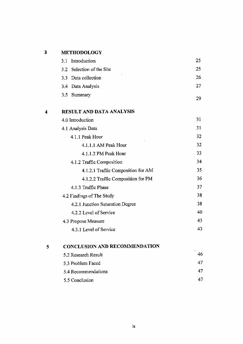
3 METHODOLOGY
3.1 Introduction 25
3.2 Selection of the Site 25
3.3 Data collection 26
3.4 Data Analysis 27
3.5 Summary29
4 RESULT AND DATA ANALYSIS
4.0 Introduction 31
4.1 Analysis Data 31
4.1.l Peak Hour 32
4.1.1.1 AM Peak Hour 32
4.1.1.2 PM Peak Hour 33
4.1.2 Traffic Composition 34
4.1.2.1 Traffic Composition for AM 35
4.1.2.2 Traffic Composition for PM 36
4.1.3 Traffic Phase 37
4.2 Findings of The Study 38
4.2.1 Junction Saturation Degree 38
4.2.2 Level of Service 40
4.3 Propose Measure 43
4.3.1 Level of Service 43
5 CONCLUSION AND RECOMMENDATION
5.2 Research Result 46
5.3 Problem Faced 47
5.4 Recommendations 47
5.5 Conclusion 47
ix
REFERENCES
APPENDICES
Appendix A Raw Data Form
Appendix B Vehicle Volumes & Adjustments
Appendix C Saturation Flowrate Determination
Appendix D Saturation Degree
Appendix E LoS Determination
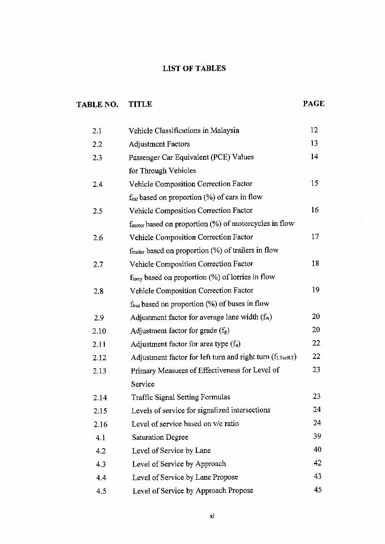
LIST OF TABLES
TABLE NO. TITLE
PAGE
2.1 Vehicle Classifications in Malaysia 12
2.2 Adjustment Factors 13
2.3 Passenger Car Equivalent (PCE) Values 14
for Through Vehicles
2.4 Vehicle Composition Correction Factor 15
fcar based on proportion (%) of cars in flow
2.5 Vehicle Composition Correction Factor 16
fmotor based on proportion (%) of motorcycles in flow
2.6 Vehicle Composition Correction Factor 17
ftraiier based on proportion (%) of trailers in flow
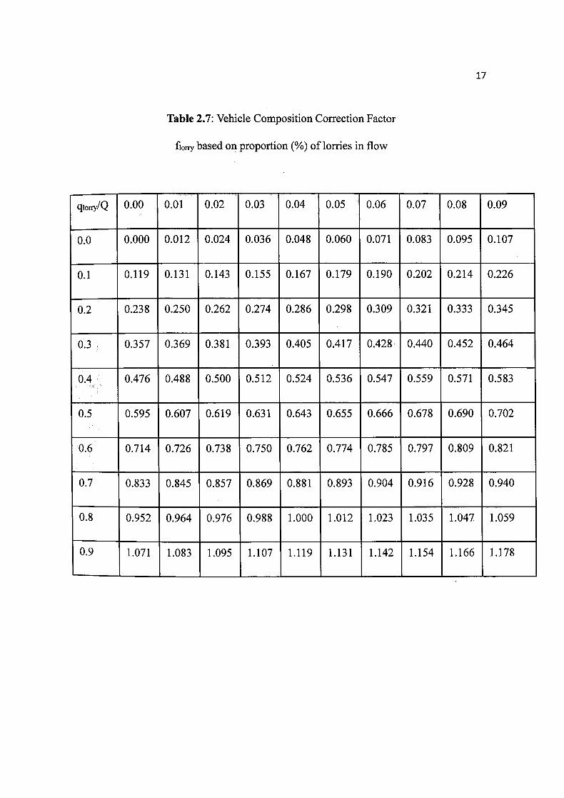
2.7 Vehicle Composition Correction Factor 18
fiorry based on proportion (%) of lorries in flow
2.8 Vehicle Composition Correction Factor 19
fbus based on proportion (%) of buses in flow
2.9 Adjustment factor for average lane width (f) 20
2.10 Adjustment factor for grade (fg) 20
2.11 Adjustment factor for area type (fa) 22
2.12 Adjustment factor for left turn and right turn (fLT0rRT) 22
2.13 Primary Measures of Effectiveness for Level of 23
Service
2.14 Traffic Signal Setting Formulas 23
2.15 Levels of service for signalized intersections 24
2.16 Level of service based on v/c ratio 24
4.1 Saturation Degree 39
4.2 Level of Service by Lane 40
4.3 Level of Service by Approach 42
4.4 Level of Service by Lane Propose 43
4.5 Level of Service by Approach Propose 45
xi
CHAPTER 1
INTRODUCTION
1.1 BACKGROUND OF STUDY
Issues on the population of Malaysia keep increasing which mean the traffic
demand also increasing. This may cause congestion in some traffic network. Traffic
congestion will causes many negative effect to the road user and environmental.
Congestion usually occurs at traffic intersection due to ineffective of traffic signal.
Traffic volume analysis must be conduct to know the traffic capacity of the junction which
is larger than traffic demand or not. Traffic demand is the total volume of vehicle using the
road network. It can be calculate by using traffic volume survey. Then, the congestion can
be classified using queue length survey to determine the delay time of the intersection.
In order to propose measures as to solve both traffic congestion and traffic queuing
problems that can alleviate traffic flow system at the intersection, the existing traffic
2
congestion problem and to quantify the volume of traffic involved at the location must be
investigate first.
1.2 PROBLEM STATEMENT
Increasing traffic demand at Kuantan town centre had made congestion at intersec-
tion of Jalan Bukit Ubi and Jalan Dato Lim Hoe Lek becoming critical and it cause
unnecessary queue for left turning movement from Jalan Bukit Ubi to Jalan Dato Lim Hoe
Lek.
1.3 SCOPE OF THE RESEARCH
This study concentrates at intersection Jalan Bukit Ubi and Jalan Dato Lim Hoe Lek
at Kuantan, Pahang. The intersection often experiences congestion due to increasing traffic
demand in Kuantan town centre. The intersection analysis using Highway Capacity
Manual. The data are collected using manual method.
1.4 OBJECTIVES
This study was conducted to achieve the following objectives:
i) To investigate the existing traffic congestion problem and to quantify the
volume of traffic involved at the location.
ii) To propose measures as to solve both traffic congestion and traffic queuing
problems that can alleviate traffic flow system at the intersection
CHAPTER 2
LITERATURE REVIEW
2.1 INTRODUCTION
Traffic congestion is a situation where the road network having higher traffic
demand than traffic capacity that be characterized by speed, travel time and queue length.
Traffic congestion not only will waste time but it also very hazardous to surrounding which
is already mention in The Public Health Costs of Traffic Congestion that is "the motor from
vehicle emission that contain pollutant that contribute outdoor air pollution".
In Traffic and Highway Engineering (2009), intersection is an area that shares by 2
or more road which in function to change direction of route. Four-leg intersection is
normally signalizing intersection. Traffic volume studies are conduct to collect data such as
number of vehicle that using the intersection in specified period. The traffic volume can be
determine the volume characteristics that we must know before designing or upgrade traffic
signal. As written in "Part 3: Traffic Studies and Analysis" in "Guide to traffic
management" (2009), there is many type of traffic survey we has such as traffic volume
survey, speed survey, travel time, queuing and delay survey, and many more.
4
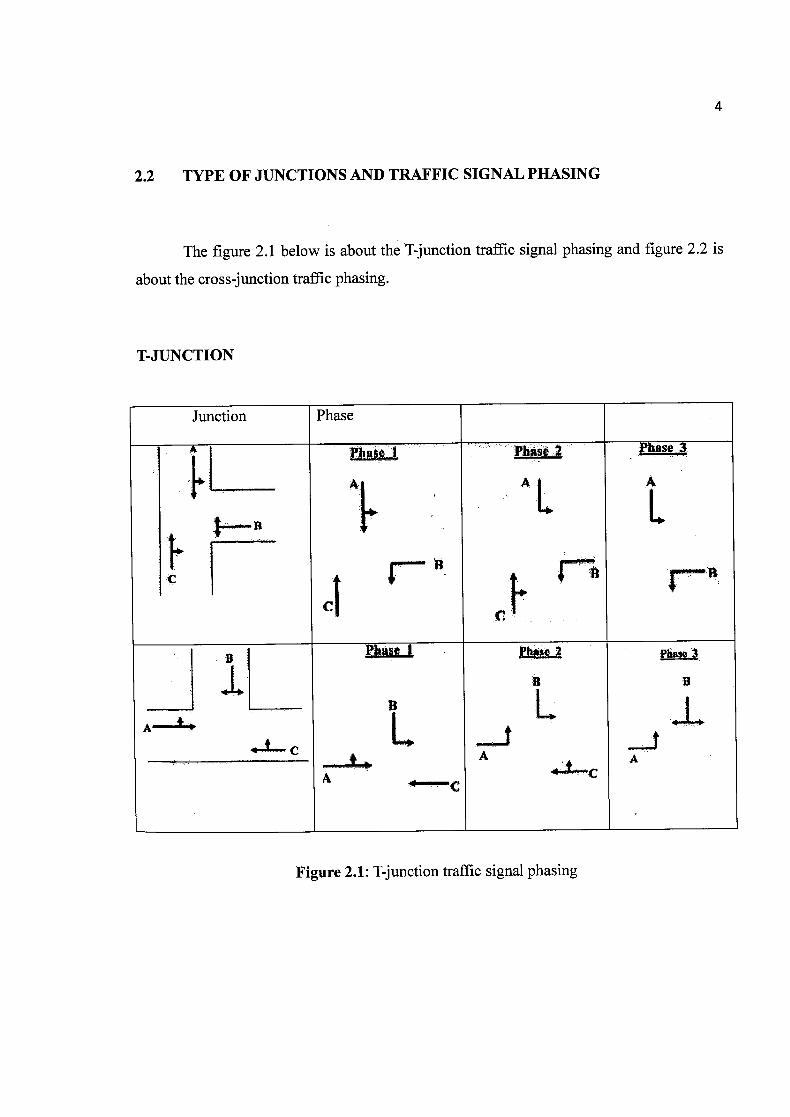
2.2 TYPE OF JUNCTIONS AND TRAFFIC SIGNAL PHASING
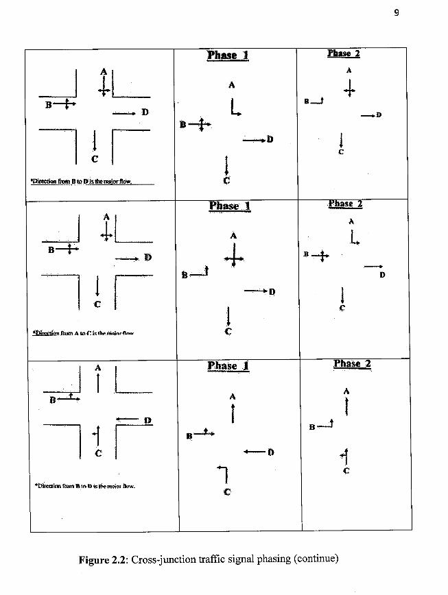
The figure 2.1 below is about the T-junction traffic signal phasing and figure 2.2 is
about the cross-junction traffic phasing.
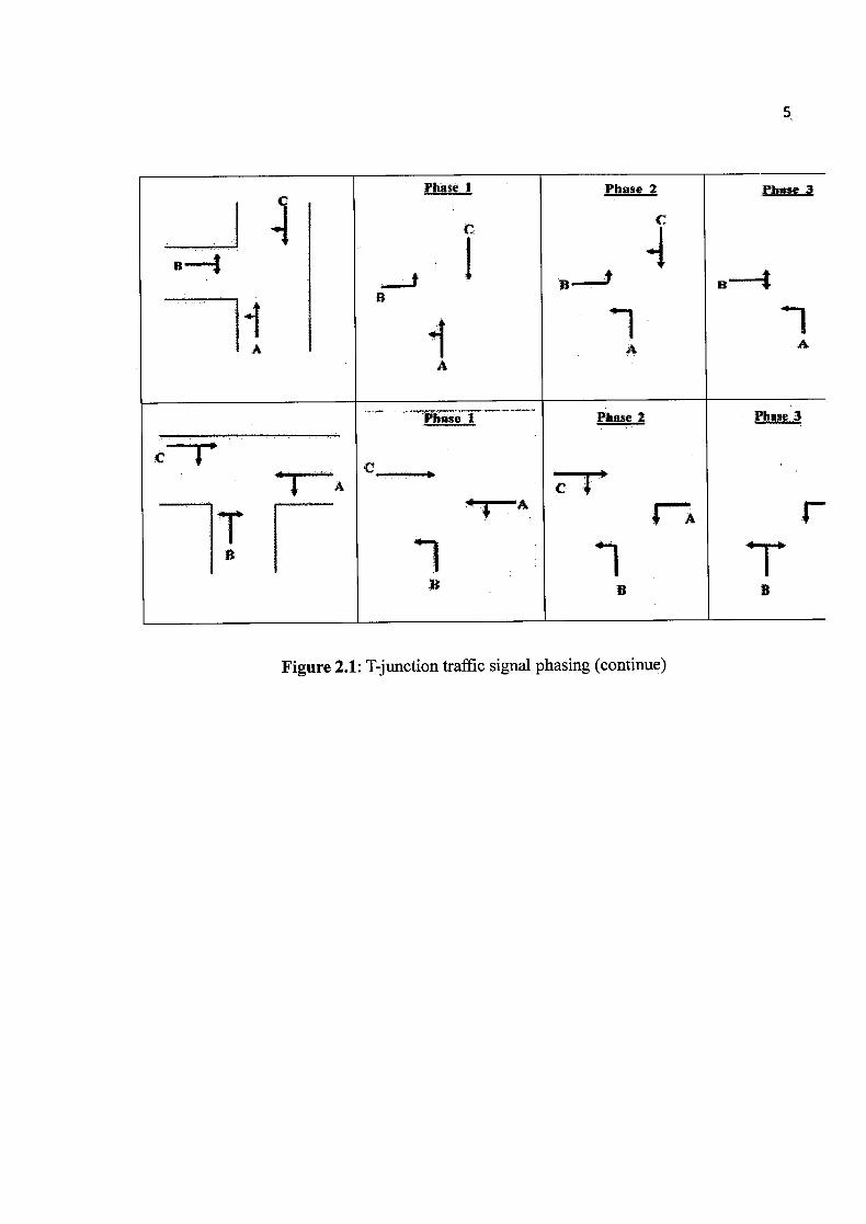
T-JUNCTION
Figure 2.1: T-j unction traffic signal phasing
Phase 3
r
-i
Figure 2.1: T-junction traffic signal phasing (continue)
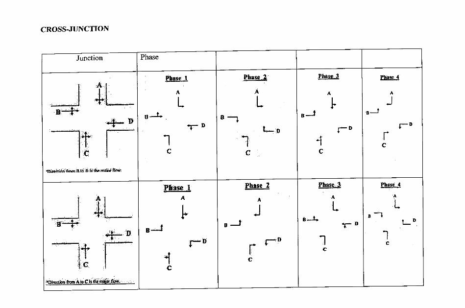
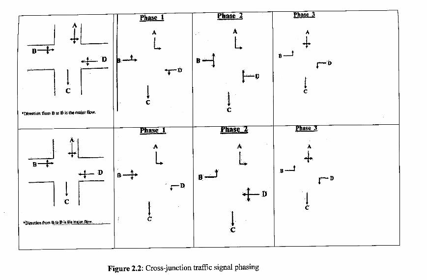
CROSS-JUNCTION
Phase3
A
çD
•1 C
Phase . a Phase 4
Phase 4
.3
D
r C
B
•Dtiin*GM B to 0 is the malor flow.
4 B__f
Figure 2.2: Cross-junction traffic signal phasing
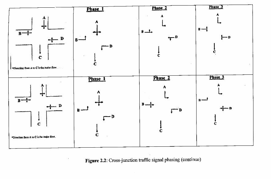
_Ph ase I Phase 1 Phase .3
F- 1.1.1 A L L -
B 4-61 D
C
aflivCct fOm A to Cis the maior flow.
Phase i Ph Phase.
A
1 c
'IIiecion A1O.i5 the miim OMC
Figure 2.2: Cross-junction traffic signal phasing (continue)
9
Figure 2.2: Cross-junction traffic signal phasing (continue)
10
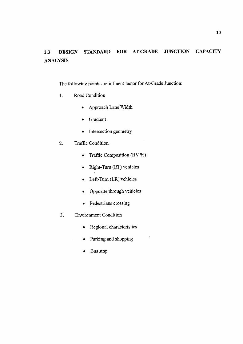
2.3 DESIGN STANDARD FOR AT-GRADE JUNCTION CAPACITY
ANALYSIS
The following points are influent factor for At-Grade Junction:
1. Road Condition
• Approach Lane Width
• Gradient
• Intersection geometry
2. Traffic Condition
• Traffic Composition (HV %)
• Right-Turn (RT) vehicles
• Left-Turn (LR) vehicles
• Opposite through vehicles
• Pedestrians crossing
3, Environment Condition
• Regional characteristics
• Parking and shopping
• Bus stop

ii.
2.4 VEHICLE CLASSIFICATION
The Table 2.1 below is shows the classification of vehicle in Malaysia for
junction analysis.
Table 2.1: Vehicle classifications in Malaysia
Class Type of vehicle
1 Passenger car, taxi, pickup and small van
2 Lorry, large van, heavy vehicle with 2 axle
3 Large lorry, trailer, heavy vehicle with 3 axles and more
4 Bus
5 Motorcycle and scooter
12
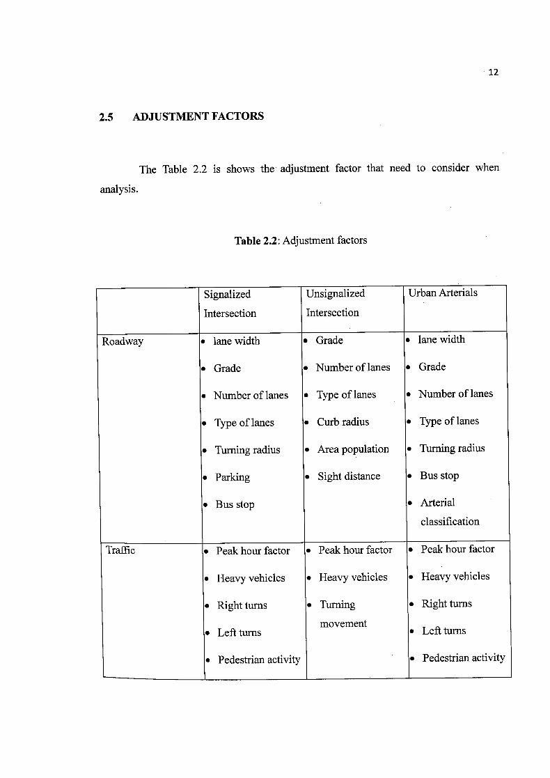
2.5 ADJUSTMENT FACTORS
The Table 2.2 is shows the adjustment factor that need to consider when
analysis.
Table 2.2: Adjustment factors
Signalized
Intersection
Unsignalized
Intersection
Urban Arterials
Roadway • lane width • Grade • lane width
• Grade • Number of lanes • Grade
• Number of lanes • Type of lanes • Number of lanes
• Type of lanes • Curb radius • Type of lanes
• Turning radius • Area population • Turning radius
• Parking • Sight distance • Bus stop
• Bus stop • Arterial
classification
Traffic • Peak hour factor • Peak hour factor • Peak hour factor
• Heavy vehicles • Heavy vehicles • Heavy vehicles
• Right turns • Turning • Right turns
• Left turnsmovement
• Left turns
• Pedestrian activity
I __
• Pedestrian activity
13
• Parking
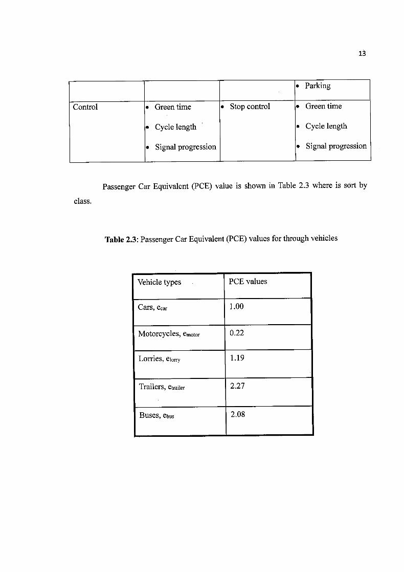
Control • Green time • Stop control • Green time
• Cycle length • Cycle length
• Signal progression • Signal progression
Passenger Car Equivalent (PCE) value is shown in Table 2.3 where is sort by
class.
Table 2.3: Passenger Car Equivalent (PCE) values for through vehicles
Vehicle types PCE values
Cars, ecar 1.00
Motorcycles, emotor 0.22
Lorries, elorry 1.19
Trailers, eaj1er 2.27
Buses, ebus 2.08
14
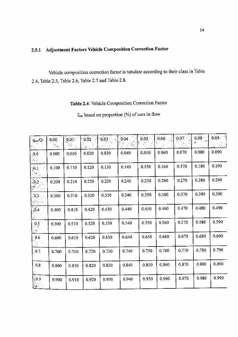
2.5.1 Adjustment Factors Vehicle Composition Correction Factor
Vehicle composition correction factor is tabulate according to their class in Table
2.4, Table 2.5, Table 2.6, Table 2.7 and Table 2.8.
Table 2.4: Vehicle Composition Correction Factor
based on proportion (%) of cars in flow
qIQ 0., , 00 001 002 003 004 005 006 007 008 009
0.0 0.000 0.010 0.020 0.030 0.040 0.050 0,060 0.070 0.080 0.090
0.1 0.100 0.110 0.120 0.130 0.140 0.150 0.160 0.170 0,180 0.190
0.2 0.200 0.210 0.220 0.230 0.240 0.250 0.260 0.270 0.280 0.290
0.3 0.300 0.310 0.320 0.330 0.340 0.350 0.360 0.370 0.380 0.390
0.4 0.400 0.410 0.420 0.430 0.440 0.450 0.460 0.470 0.480 0.490
0.5 0.500 0.510 0.520 0.530 0.540 0.550 0.560 0.570 0.580 0.590
0,6 0.600 0.610 0.620 0.630 0.640 0.650 0.660 0.670 0.680 0.690
0.7 0.700 0.710 0.720 0.730 0.740 0.750 0.760 0.770 0.780 0.790
0.8 0.800 0.810 0.820 0.830 0.840 0.850 0.860 0.870 0.880 0.890
0.9 0.900 0.910 0.920 0.930 0.940 0.950 0.960 0.970 0.980 0.990
15
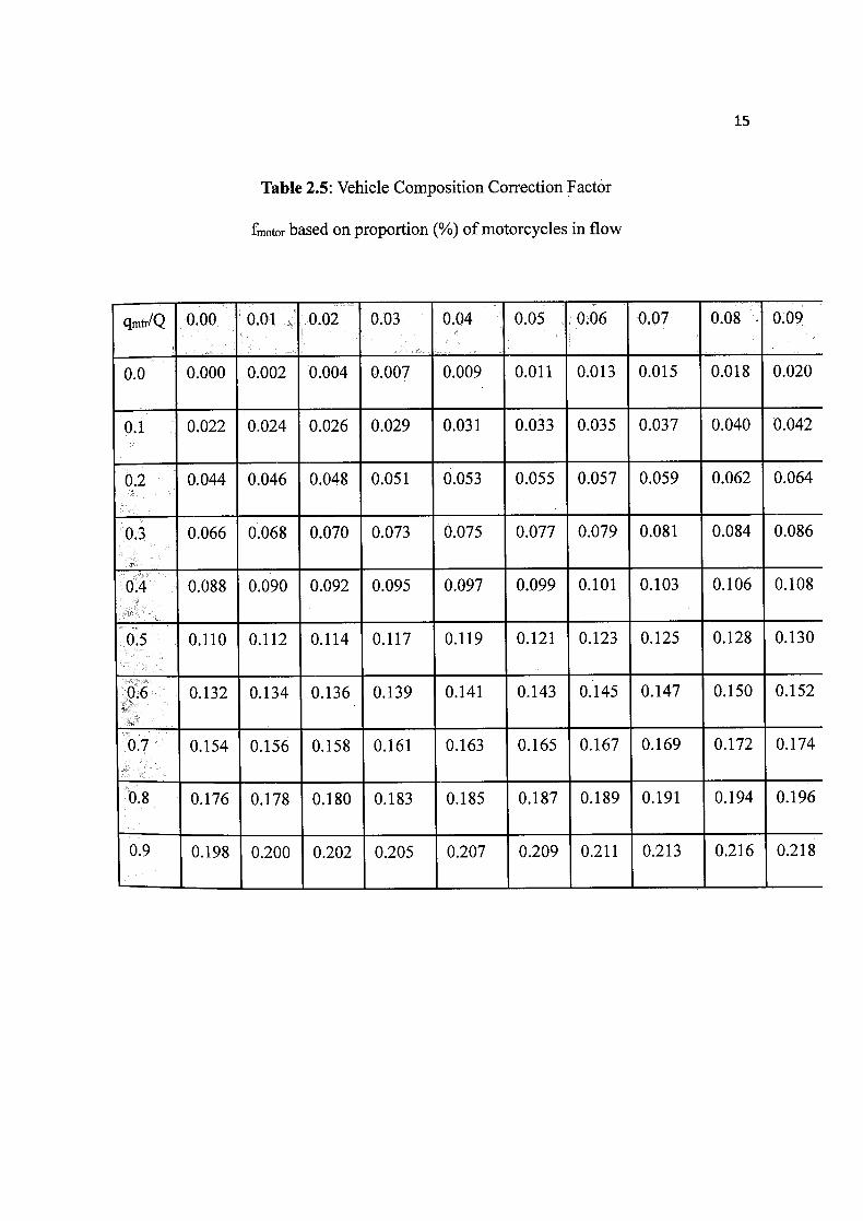
Table 2.5: Vehicle Composition Correction Factor
fmotor based on proportion (%) of motorcycles in flow
qmtr/Q 000 001 002 003 004 005 006 007 008 009
0.0 0.000 0.002 0.004 0.007 0.009 0.011 0.013 0.015 0.018 0.020
0.1 0.022 0,024 0.026 0.029 0.031 0.033 0.035 0.037 0.040 0.042
02 0.044 0.046 0.048 0.051 0.053 0.055 0.057 0.059 0.062 0.064
03 0.066 0.068 0.070 0.073 0.075 0.077 0.079 0.081 0.084 0.086
0.4 0.088 0.090 0.092 0.095 0.097 0.099 0.101 0.103 0.106 0.108
0.5 0.110 0.112 0.114 0.117 0.119 0.121 0.123 0.125 0.128 0.130
0.6 0.132 0.134 0.136 0.139 0.141 0.143 0.145 0.147 0.150 0.152
0.7 0.154 0.156 0.158 0.161 0.163 0.165 0.167 0.169 0.172 0.174
0.8 0.176 0.178 0.180 0.183 0.185 0.187 0.189 0.191 0.194 0.196
0.9 0.198 0.200 0.202 0.205 0.207 0.209 0.211 0.213 0.216 0.218
16
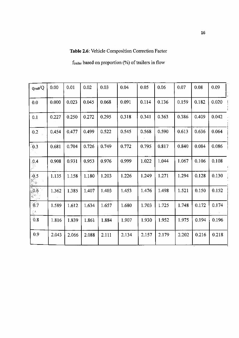
Table 2.6: Vehicle Composition Correction Factor
ftraiier based on proportion (%) of trailers in flow
qtraii/Q 0.00 0.01 0.02 0.03 0.04 0.05 0.06 0.07 0.08 0.09
0.0 0.000 0.023 0.045 0.068 0.091 0.114 0.136 0.159 0.182 0.020
0.1 0.227 0.250 0.272 0.295 0.318 0.341 0.363 0.386 0.409 0.042
0.2 0.454 0.477 0.499 0.522 0.545 0.568 0.590 0.613 0.636 0.064
03 0.681 0.704 0.726 0.749 0.772 0.795 0.817 0.840 0.084 0.086
0.4 0.908 0.931 0.953 0.976 0.999 1.022 1.044 1.067 0.106 0.108
0.5 1.135 1.158 1.180 1.203 1.226 1.249 1.271 1.294 0.128 0.130
0.6 1.362 1.385 1.407 1.403 1.453 1.476 1.498 1.521 0.150 0.152
0.7 1.589 1.612 1.634 1.657 1.680 1.703 1.725 1.748 0.172 0.174
0.8 1.816 1.839 1.861 1.884 1.907 1.930 1.952 1.975 0.194 0.196
0.9 2.043 2.066 2.088 2.111 2.134 2.157 2.179 2.202 0.216 0.218
17
Table 2.7: Vehicle Composition Correction Factor
fi0 based on proportion (%) of lorries in flow
qiorry/Q
-
0.00 0.01 0.02 0.03 0.04 0.05 0.06 0.07 0.08 0.09
0.0 0.000 0.012 0.024 0.036 0.048 0.060 0.071 0.083 0.095 0.107
0.1 0.119 0.131 0.143 0.155 0.167 0.179 0.190 0.202 0.214 0.226
0.2 0.238 0.250 0,262 0.274 0.286 0.298 0.309 0.321 0.333 0.345
0.3 0.357 0.369 0.381 0.393 0.405 0.417 0.428 0.440 0.452 0.464
0.4 0.476 0.488 0.500 0.512 0.524 0.536 0.547 0.559 0.571 0.583
0.5 0.595 0.607 0.619 0.631 0.643 0.655 0.666 0.678 0.690 0.702
0.6 0.714 0.726 0.738 0.750 0.762 0.774 0.785 0.797 0.809 0.821
0.7 0.833 0.845 0.857 0.869 0.881 0.893 0.904 0.916 0.928 0.940
0.8 0.952 0.964 0.976 0.988 1.000 1.012 1.023 1.035 1.047 1.059
0.9 1.071 1.083 1.095 1.107 1.119 1.131 1.142 1.154 1.166 1.178