11.1 + 11.2. Copyright © 2013, 2010 and 2007 Pearson Education, Inc. Section Inference about Two Population Proportions 11.1

11.1 + 11.2

Copyright © 2013, 2010 and 2007 Pearson Education, Inc.

Section

Inference about Two Population Proportions

11.1


For each of the following, determine whether the sampling method is independent or dependent.

a)A researcher wants to know whether the price of a one night stay at a Holiday Inn Express is less than the price of a one night stay at a Red Roof Inn. She randomly selects 8 towns where the location of the hotels is close to each other and determines the price of a one night stay.

b)A researcher wants to know whether the “state” quarters (introduced in 1999) have a mean weight that is different from “traditional” quarters. He randomly selects 18 “state” quarters and 16 “traditional” quarters and compares their weights.

Parallel Example 1: Distinguish between Independent and Dependent Sampling

11-3


a) The sampling method is dependent since the 8 Holiday Inn Express hotels can be matched with one of the 8 Red Roof Inn hotels by town.

b) The sampling method is independent since the “state” quarters which were sampled had no bearing on which “traditional” quarters were sampled.

Solution

11-4


Suppose that a simple random sample of size n1 is taken from a

population where x1 of the individuals have a specified

characteristic, and a simple random sample of size n2 is

independently taken from a different population where x2 of the

individuals have a specified characteristic. The sampling

distribution of , where and , is

approximately normal, with mean and standard

deviation

provided that and and

each sample size is no more than 5% of the population size.

Sampling Distribution of the Difference between Two Proportions (Independent Sample)

ˆ p 1 ˆ p 2

ˆ p 1 x1 n1

ˆ p 1 ˆ p 2p1 p2

ˆ p 2 x2 n2

ˆ p 1 ˆ p 2

p1 1 p1 n1

p2 1 p2

n2

n1ˆ p 1 1 ˆ p 1 10

n2ˆ p 2 1 ˆ p 2 10

11-5


The standardized version of is then written as

which has an approximate standard normal distribution.

Sampling Distribution of the Difference between Two Proportions

ˆ p 1 ˆ p 2

Z ˆ p 1 ˆ p 2 p1 p2

p1 1 p1 n1

p2 1 p2

n2

11-6


The best point estimate of p is called the pooled estimate of p, denoted , where

Test statistic for Comparing Two Population Proportions

ˆ p

ˆ p x1 x2

n1 n2

z0 ˆ p 1 ˆ p 2 ˆ p 1 ˆ p 2

ˆ p 1 ˆ p 2

ˆ p 1 ˆ p 1

n1

1

n2

11-7


To test hypotheses regarding two population proportions, p1 and p2, we can use the steps that follow, provided that:

the samples are independently obtained using simple random sampling,

and and n1 ≤ 0.05N1 and n2 ≤ 0.05N2 (the sample size is

no more than 5% of the population size); this requirement ensures the independence necessary for a binomial experiment.

Hypothesis Test Regarding the Differencebetween Two Population Proportions

n1ˆ p 1 1 ˆ p 1 10

n2ˆ p 2 1 ˆ p 2 10,

11-8


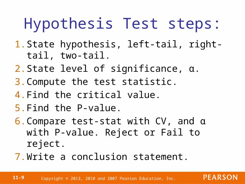
Hypothesis Test steps:1. State hypothesis, left-tail, right-tail, two-tail.

2. State level of significance, α.

3. Compute the test statistic.

4. Find the critical value.

5. Find the P-value.

6. Compare test-stat with CV, and α with P-value. Reject or Fail to reject.

7. Write a conclusion statement.

11-9


Step 3: Compute the test statistic

where

1 2

0

1 2

ˆ ˆ

1 1ˆ ˆ1

p pz

p pn n

1 2

1 2

ˆ .x x

pn n

Classical Approach

11-10


Technology Step 3: Use a statistical spreadsheet or calculator with statistical capabilities to obtain the P-value. The directions for obtaining the P-value using the TI-83/84 Plus graphing calculator, Excel, MINITAB, and StatCrunch are in the Technology Step-by-Step in the text.

P-Value Approach

11-11


An economist believes that the percentage of urban households with Internet access is greater than the percentage of rural households with Internet access. He obtains a random sample of 800 urban households and finds that 338 of them have Internet access. He obtains a random sample of 750 rural households and finds that 292 of them have Internet access. Test the economist’s claim at the α = 0.05 level of significance.

Parallel Example 1: Testing Hypotheses Regarding Two Population Proportions

11-12


We must first verify that the requirements are satisfied:

1. The samples are simple random samples that were obtained independently.

2. x1=338, n1=800, x2=292 and n2=750, so

3. The sample sizes are less than 5% of the population size.

Solution

ˆ p 1 338

8000.4225 and ˆ p 2

292

7500.3893. Thus,

n1ˆ p 1 1 ˆ p 1 800(0.4225)(1 0.4225) 195.195 10

n2ˆ p 2 1 ˆ p 2 750(0.3893)(1 0.3893) 178.309 10

11-13


Step 1: We want to determine whether the percentage of urban households with Internet access is greater than the percentage of rural households with Internet access. So,

H0: p1 = p2 versus H1: p1 > p2

or, equivalently,

H0: p1 - p2=0 versus H1: p1 - p2 > 0

Step 2: The level of significance is α = 0.05.

Solution

11-14


Step 3: The pooled estimate of is:

The test statistic is:

Solution

z0 0.4225 0.3893

0.4065 1 0.4065 1

800 1

750

1.33.

ˆ p

ˆ p x1 x2

n1 n2

338 292

800 7500.4065.

11-15


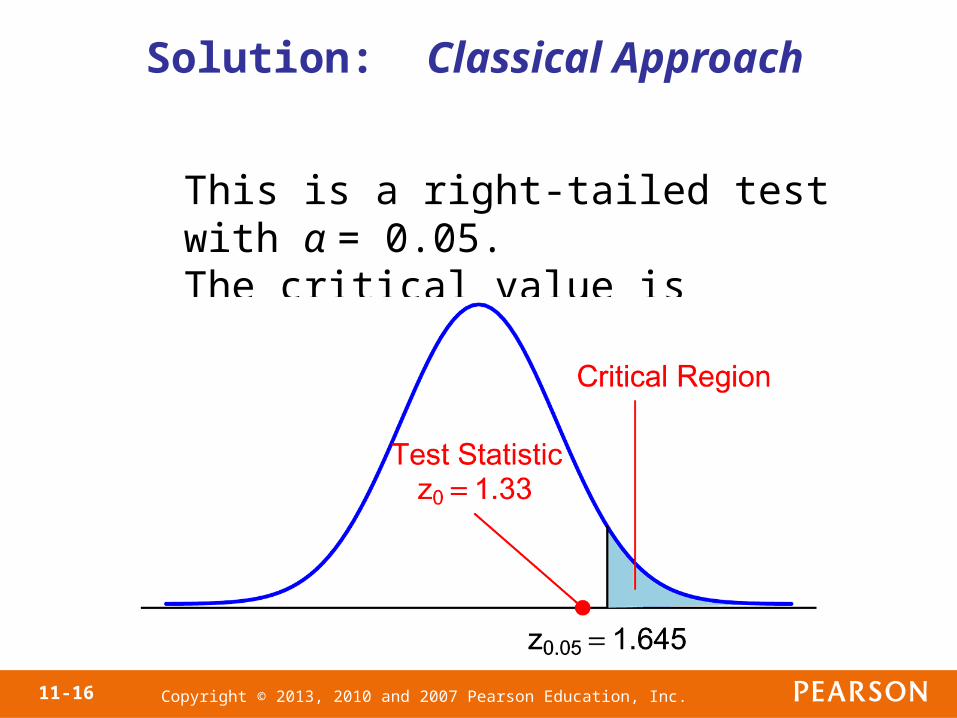
This is a right-tailed test with α = 0.05.The critical value is z0.05=1.645.

Solution: Classical Approach

11-16


Step 4: Since the test statistic, z0=1.33 is less than the critical value z.05=1.645, we fail to reject the null hypothesis.


11-17


Because this is a right-tailed test, the P-value is the area under the normal to the right of the test statistic z0=1.33.That is, P-value = P(Z > 1.33) ≈ 0.09.

Solution: P-Value Approach

11-18


Step 4: Since the P-value is greater than the level of significance α = 0.05, we fail to reject the null hypothesis.


11-19


Step 5: There is insufficient evidence at the α = 0.05 level to conclude that the percentage of urban households with Internet access is greater than the percentage of rural households with Internet access.

Solution

11-20


Objective 3

• Construct and Interpret Confidence Intervals for the Difference between Two Population Proportions

11-21


To construct a (1 – α)•100% confidence interval for the difference between two population proportions, the following requirements must be satisfied:

1. the samples are obtained independently using simple random sampling,

2. , and

3. n1 ≤ 0.05N1 and n2 ≤ 0.05N2 (the sample size is no more than 5% of the population size); this requirement ensures the independence necessary for a binomial experiment.

Constructing a (1 – α)•100% Confidence Interval for the Difference between Two

Population Proportions

n1ˆ p 1 1 ˆ p 1 10

n2ˆ p 2 1 ˆ p 2 10

11-22


Provided that these requirements are met,a (1 – α)•100% confidence interval for p1–p2 is given by

Lower bound:

Upper bound:

ˆ p 1 ˆ p 2 z2

ˆ p 1 1 ˆ p 1

n1

ˆ p 2 1 ˆ p 2

n2

ˆ p 1 ˆ p 2 z2

ˆ p 1 1 ˆ p 1

n1

ˆ p 2 1 ˆ p 2

n2

Constructing a (1 – α)•100% Confidence Interval for the Difference between Two

Population Proportions

11-23


An economist obtains a random sample of 800 urban households and finds that 338 of them have Internet access. He obtains a random sample of 750 rural households and finds that 292 of them have Internet access. Find a 99% confidence interval for the difference between the proportion of urban households that have Internet access and the proportion of rural households that have Internet access.

Parallel Example 3: Constructing a Confidence Interval for the Difference between Two Population Proportions

11-24


We have already verified the requirements for constructing a confidence interval for the difference between two population proportions in the previous example.

Recall

Solution

ˆ p 1 338

8000.4225 and ˆ p 2

292

7500.3893.

11-25


Thus,

Lower bound =

Upper bound =

Solution

0.4225 0.3893

2.5750.4225(1 0.4225)

800

0.3893(1 0.3893)

750 0.0310

0.4225 0.3893

2.5750.4225(1 0.4225)

800

0.3893(1 0.3893)

7500.0974

11-26


We are 99% confident that the difference between the proportion of urban households that have Internet access and the proportion of rural households that have Internet access is between –0.03 and 0.10. Since the confidence interval contains 0, we are unable to conclude that the proportion of urban households with Internet access is greater than the proportion of rural households with Internet access.

Solution

11-27


Objective 4

• Test Hypotheses Regarding Two Proportions from Dependent Samples

11-28


McNemar’s Test is a test that can be used to compare two proportions with matched-pairs data (i.e., dependent samples)

11-29


Testing a Hypothesis Regarding the Difference of Two Population

Proportions: Dependent Samples

To test hypotheses regarding two population proportionsp1 and p2, where the samples are dependent, arrange thedata in a contingency table as follows:

Treatment A

Treatment B

Success Failure

Success f11 f12

Failure f21 f22

11-30


Testing a Hypothesis Regarding the Difference of Two Population

Proportions: Dependent Samples

We can use the steps that follow provided that:1. the samples are dependent and are obtained

randomly and2. the total number of observations where the

outcomes differ must be greater than or equal to 10.That is, f12 + f21 ≥ 10.

11-31









11-32


Step 1: Determine the null and alternative hypotheses.

H0: the proportions between the two populations are equal (p1 = p2)

H1: the proportions between the two populations differ (p1 ≠ p2)

11-33



z0 f12 f21 1

f12 f21

11-34


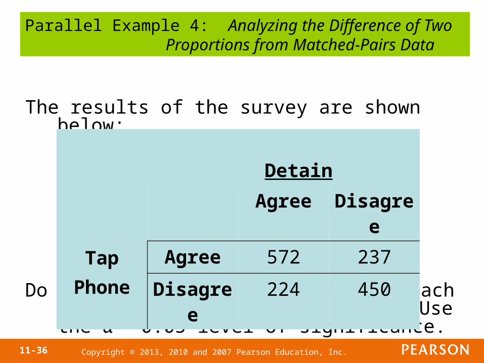
A recent General Social Survey asked the following two questions of a random sample of 1483 adult Americans under the hypothetical scenario that the government suspected that a terrorist act was about to happen:

• Do you believe the authorities should have the right to tap people’s telephone conversations?

• Do you believe the authorities should have the right to detain people for as long as they want without putting them on trial?

Parallel Example 4: Analyzing the Difference of Two Proportions from Matched-Pairs Data

11-35


The results of the survey are shown below:

Do the proportions who agree with each scenario differ significantly? Use the α = 0.05 level of significance.

Parallel Example 4: Analyzing the Difference of Two Proportions from Matched-Pairs Data

Detain

TapPhone

Agree Disagree

Agree 572 237

Disagree 224 450

11-36


The sample proportion of individuals who believe that

the authorities should be able to tap phones is

.

The sample proportion of individuals who believe that

the authorities should have the right to detain people is

. We want to determine

whether the difference in sample proportions is due to

sampling error or to the fact that the population

proportions differ.

Solution

ˆ p T 572 237

14830.5455

ˆ p D 572 224

14830.5367

11-37


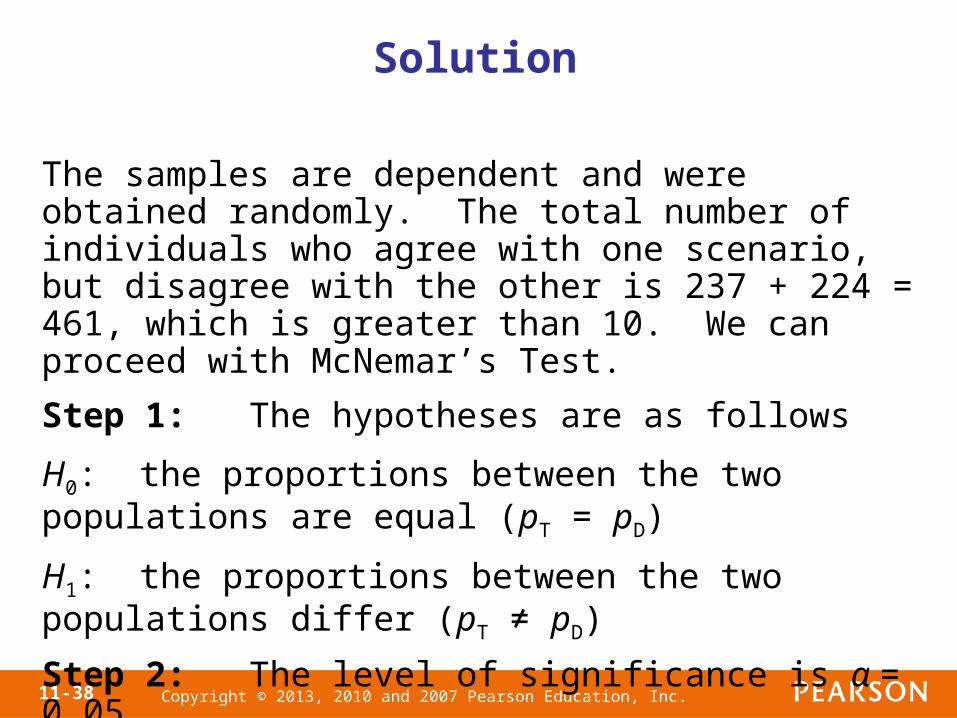
The samples are dependent and were obtained randomly. The total number of individuals who agree with one scenario, but disagree with the other is 237 + 224 = 461, which is greater than 10. We can proceed with McNemar’s Test.

Step 1: The hypotheses are as follows

H0: the proportions between the two populations are equal (pT = pD)

H1: the proportions between the two populations differ (pT ≠ pD)


Solution

11-38


Step 3: The test statistic is:

Solution

z0 224 237 1

237 2240.56

11-39


The critical value with an α = 0.05 level of significance is z0.025 = 1.96.


11-40


Step 4: Since the test statistic, z0 = 0.56 is less than the critical value z.025 = 1.96, we fail to reject the null hypothesis.


11-41


The P-value is two times the area under the normal curve to the right of the test statistic z0=0.56.That is, P-value = 2•P(Z > 0.56) ≈ 0.5754.


11-42


Step 4: Since the P-value is greater than the level of significance α = 0.05, we fail to reject the null hypothesis.


11-43


Step 5: There is insufficient evidence at the α = 0.05 level to conclude that there is a difference in the proportion of adult Americans who believe it is okay to phone tap versus detaining people for as long as they want without putting them on trial in the event that the government believed a terrorist plot was about to happen.

Solution

11-44


Objective 5

• Determine the Sample Size Necessary for Estimating the Difference between Two Population Proportions within a Specified Margin of Error

11-45


Sample Size for Estimating p1 – p2

The sample size required to obtain a (1 – α)•100% confidence interval with a margin of error, E, is givenby

rounded up to the next integer, if prior estimates of p1

and p2, , are available. If prior estimates ofp1 and p2 are unavailable, the sample size is

rounded up to the next integer.

p̂1 and p̂2

n n1 n2 0.5z 2

E

2

11-46


A doctor wants to estimate the difference in the proportion of 15-19 year old mothers that received prenatal care and the proportion of 30-34 year old mothers that received prenatal care. What sample size should be obtained if she wished the estimate to be within 2 percentage points with 95% confidence assuming:

a)she uses the results of the National Vital Statistics Report results in which 98% of the 15-19 year old mothers received prenatal care and 99.2% of 30-34 year old mothers received prenatal care.

b)she does not use any prior estimates.

Parallel Example 5: Determining Sample Size

11-47


We have E = 0.02 and zα/2 = z0.025 = 1.96.

a) Letting ,

The doctor must sample 265 randomly selected 15-19 year old mothers and 265 randomly selected 30-34 year old mothers.

Solution

ˆ p 1 0.98 and ˆ p 2 0.992

n1 n2 0.98(1 0.98) 0.992(1 0.992) 1.96

0.02

2

264.5

11-48


b) Without prior estimates of p1 and p2, the sample size is

The doctor must sample 4802 randomly selected 15-19 year old mothers and 4802 randomly selected 30-34 year old mothers. Note that having prior estimates of p1 and p2 reduces the number of mothers that need to be surveyed.

Solution

n1 n2 0.51.96

0.02

2

4802

11-49


Section

Inference about Two Means: Dependent Samples

11.2


Objectives

1. Test hypotheses regarding matched-pairs data

2. Construct and interpret confidence intervals about the population mean difference of matched-pairs data

11-51


“In Other Words”

Statistical inference methods on matched-pairs data use the same methods as inference on a single population mean, except that the differences are analyzed.

11-52


To test hypotheses regarding the mean difference of matched-pairs data, the following must be satisfied:

•the sample is obtained using simple random sampling

•the sample data are matched pairs,

•the differences are normally distributed with no outliers or the sample size, n, is large (n ≥ 30).

Testing Hypotheses Regarding the Differenceof Two Means Using a Matched-Pairs Design

11-53


Step 1: Determine the null and alternative hypotheses. The hypotheses can be structured in one of three ways, where μd is the population mean difference of the matched-pairs data.

11-54









11-55



which approximately follows Student’s t-distribution with n – 1 degrees of freedom. The values of and sd are the mean and standard deviation of the differenced data.

d

t0

d

sd

n

Classical Approach

11-56



which approximately follows Student’s t-distribution with n – 1 degrees of freedom. The values of and sd are the mean and standard deviation of the differenced data.

d

t0

d

sd

n

P-Value Approach

11-57


Technology Step 3:Use a statistical spreadsheet or calculator with statistical capabilities to obtain the P-value. The directions for obtaining the P-value using the TI-83/84 Plus graphing calculator, MINITAB, Excel and StatCrunch, are in the Technology Step-by-Step on page in the text.

P-Value Approach

11-58


These procedures are robust, which means that minor departures from normality will not adversely affect the results. However, if the data have outliers, the procedure should not be used.

11-59


The following data represent the cost of a one night stay in Hampton Inn Hotels and La Quinta Inn Hotels for a random sample of 10 cities. Test the claim that Hampton Inn Hotels are priced differently than La Quinta Hotels at the α = 0.05 level of significance.

Parallel Example 2: Testing a Claim Regarding Matched-Pairs Data

11-60


City Hampton Inn La Quinta

Dallas 129 105

Tampa Bay 149 96

St. Louis 149 49

Seattle 189 149

San Diego 109 119

Chicago 160 89

New Orleans 149 72

Phoenix 129 59

Atlanta 129 90

Orlando 119 69

11-61


This is a matched-pairs design since the hotel prices come from the same ten cities. To test the hypothesis, we first compute the differences and then verify that the differences come from a population that is approximately normally distributed with no outliers because the sample size is small.

The differences (Hampton - La Quinta) are:

24 53 100 40 –10 71 77 70 39 50

with = 51.4 and sd = 30.8336.

Solution

d

11-62


No violation of normality assumption.

Solution

11-63


No outliers.

Solution

11-64


Step 1: We want to determine if the prices differ:

H0: μd = 0 versus H1: μd ≠ 0


Step 3: The test statistic is

Solution

t0 51.4

30.833610

5.2716.

11-65


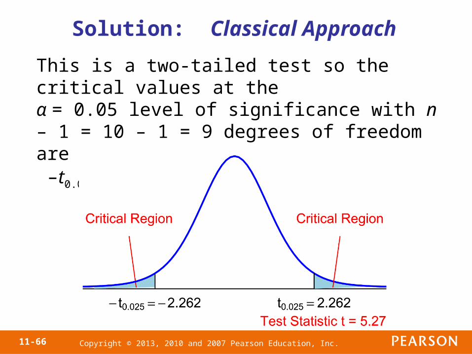
This is a two-tailed test so the critical values at theα = 0.05 level of significance with n – 1 = 10 – 1 = 9 degrees of freedom are –t0.025 = –2.262 and t0.025 = 2.262.


11-66


Step 4: Since the test statistic, t0 = 5.27 is greater than the critical value t.025 = 2.262, we reject the null hypothesis.


11-67


Because this is a two-tailed test, the P-value is two times the area under the t-distribution withn – 1 = 10 – 1 = 9 degrees of freedom to the right of the test statistic t0 = 5.27.That is, P-value = 2P(t > 5.27) ≈ 2(0.00026) = 0.00052 (using technology). Approximately 5 samples in 10,000 will yield results as extreme as we obtained if the null hypothesis is true.


11-68


Step 4: Since the P-value is less than the level of significance α = 0.05, we reject the null hypothesis.


11-69


Step 5: There is sufficient evidence to conclude that Hampton Inn hotels and La Quinta hotels are priced differently at the α = 0.05 level of significance.

Solution

11-70


Objective 2

• Construct and Interpret Confidence Intervals for the Population Mean Difference of Matched-Pairs Data

11-71


A (1 – α)•100% confidence interval for μd is given by

Lower bound:

Upper bound:

The critical value tα/2 is determined using n – 1 degrees of freedom. The values of and sd are the mean and standard deviation of the differenced data.

Confidence Interval for Matched-Pairs Data

d t

2

s

d

n

d

d t

2

s

d

n

11-72


Note: The interval is exact when the population is normally distributed and approximately correct for nonnormal populations, provided that n is large.

Confidence Interval for Matched-Pairs Data

11-73


Construct a 90% confidence interval for the mean difference in price of Hampton Inn versus La Quinta hotel rooms.

Parallel Example 4: Constructing a Confidence Interval for Matched-Pairs Data

11-74


• We have already verified that the differenced data come from a population that is approximately normal with no outliers.

• Recall = 51.4 and sd = 30.8336.

• From Table VI with α = 0.10 and 9 degrees of freedom, we find tα/2 = 1.833.

Solution

d

11-75


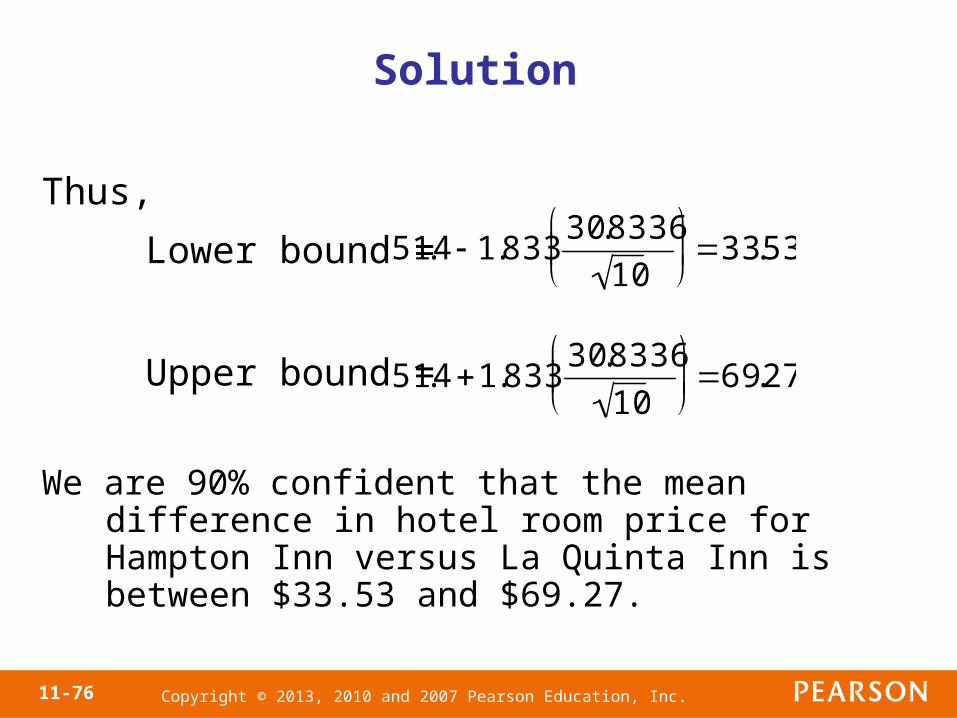
Thus,

• Lower bound =

• Upper bound =

We are 90% confident that the mean difference in hotel room price for Hampton Inn versus La Quinta Inn is between $33.53 and $69.27.

Solution

51.4 1.83330.8336

10

33.53

51.4 1.83330.8336

10

69.27

11-76

Documents

11.1 + 11.2. Copyright © 2013, 2010 and 2007 Pearson Education, Inc. Section Inference about Two Population Proportions 11.1