Embed Size (px)
Citation preview

110 Notes on Numerical Fluid Mechanics and Multidisciplinary Design (NNFM)
EditorsW. Schröder/Aachen
B.J. Boersma/DelftK. Fujii/Kanagawa
W. Haase/MünchenM.A. Leschziner/London
J. Periaux/ParisS. Pirozzoli/Rome
A. Rizzi/StockholmB. Roux/Marseille
Y. Shokin/Novosibirsk

Turbulence and InteractionsProceedings the TI 2009 Conference
Michel DevilleThien-Hiep LêPierre Sagaut(Editors)
ABC
Prof. Michel DevilleEPFL STI IGM LINStation 91015 LausanneSwitzerlandE-mail: [email protected]
Dr. Thien-Hiep LêONERA29 Avenue de la Division Leclerc92322 ChatillonFrance
Prof. Pierre SagautInstitut Jean Le Rond d’AlembertUniversité Pierre et Marie Curie4 Place Jussieu75252 Paris cedex 5France
ISBN 978-3-642-14138-6 e-ISBN 978-3-642-14139-3
DOI 10.1007/978-3-642-14139-3
Notes on Numerical Fluid Mechanicsand Multidisciplinary Design ISSN 1612-2909
Library of Congress Control Number: 2010929478
c© 2010 Springer-Verlag Berlin Heidelberg
This work is subject to copyright. All rights are reserved, whether the whole or part of the material isconcerned, specifically the rights of translation, reprinting, reuse of illustrations, recitation, broadcasting,reproduction on microfilm or in any other way, and storage in data banks. Duplication of this publicationor parts thereof is permitted only under the provisions of the German Copyright Law of September 9,1965, in its current version, and permission for use must always be obtained from Springer. Violationsare liable for prosecution under the German Copyright Law.
The use of general descriptive names, registered names, trademarks, etc. in this publication does notimply, even in the absence of a specific statement, that such names are exempt from the relevant protectivelaws and regulations and therefore free for general use.
Typeset & Cover Design: Scientific Publishing Services Pvt. Ltd., Chennai, India.
Printed on acid-free paper
5 4 3 2 1 0
springer.com

NNFM Editor Addresses
Prof. Dr. Wolfgang Schröder(General Editor)RWTH AachenLehrstuhl für Strömungslehre undAerodynamisches InstitutWüllnerstr. 5a52062 AachenGermanyE-mail: [email protected]
Prof. Dr. Kozo FujiiSpace Transportation Research DivisionThe Institute of Spaceand Astronautical Science3-1-1, Yoshinodai, SagamiharaKanagawa, 229-8510JapanE-mail: [email protected]
Dr. Werner HaaseHöhenkirchener Str. 19dD-85662 HohenbrunnGermanyE-mail: [email protected]
Prof. Dr. Ernst Heinrich Hirschel(Former General Editor)Herzog-Heinrich-Weg 6D-85604 ZornedingGermanyE-mail: [email protected]
Prof. Dr. Ir. Bendiks Jan BoersmaChair of EnergytechnologyDelft University of TechnologyLeeghwaterstraat 442628 CA DelftThe NetherlandsE-mail: [email protected]
Prof. Dr. Michael A. LeschzinerImperial College of ScienceTechnology and MedicineAeronautics DepartmentPrince Consort RoadLondon SW7 2BYU.K.E-mail: [email protected]
Prof. Dr. Sergio PirozzoliUniversità di Roma “La Sapienza”Dipartimento di Meccanica e AeronauticaVia Eudossiana 1800184, Roma, ItalyE-mail: [email protected]
Prof. Dr. Jacques Periaux38, Boulevard de ReuillyF-75012 ParisFranceE-mail: [email protected]
Prof. Dr. Arthur RizziDepartment of AeronauticsKTH Royal Institute of TechnologyTeknikringen 8S-10044 StockholmSwedenE-mail: [email protected]
Dr. Bernard RouxL3M – IMT La JetéeTechnopole de Chateau-GombertF-13451 Marseille Cedex 20FranceE-mail: [email protected]
Prof. Dr. Yurii I. ShokinSiberian Branch of theRussian Academy of SciencesInstitute of ComputationalTechnologiesAc. Lavrentyeva Ave. 6630090 NovosibirskRussiaE-mail: [email protected]

Preface
The “Turbulence and Interactions 2009” (TI2009) conference was held in Saint-Luce on the island of La Martinique, France, on May 31-June 5, 2009. The scien-tific sponsors of the conference were
• DGA • Ecole Polytechnique Fédérale de Lausanne (EPFL), • ERCOFTAC : European Research Community on Flow, Turbulence and
Combustion, • Institut Jean Le Rond d’Alembert, Paris, • ONERA.
This second TI conference was very successful as it attracted 65 researchers from 17 countries. The magnificent venue and the beautiful weather helped the participants to discuss freely and casually, share ideas and projects, and spend very good times all together.
The organisers were fortunate in obtaining the presence of the following in-vited speakers: L. Fuchs (KTH, Stockholm and Lund University), J. Jimenez (Univ. Politecnica Madrid), C.-H. Moeng (NCAR), A. Scotti (University of North Carolina), L. Shen (Johns Hopkins University) and A.J. Smits (Princeton Univer-sity). The topics covered by the 62 contributed papers ranged from experimental results through theory to computations. They represent a snapshot of the state-of-the-art in turbulence research. The papers of the conference went through the usual reviewing process and the result is given in this book of Proceedings.
In the present volume, the reader will find the keynote lectures followed by the contributed talks given in alphabetical order of the first author.
The organizers of the conference would like to acknowledge the support of EPFL, Université Pierre et Marie Curie, Paris and ONERA. They express their gratitude for their colleagues of the organizing committee, especially Drs. V. Gle-ize and M. Terracol, for their help and constant efficiency.
Lausanne, Paris December 3, 2009
M. O. Deville T. H. Lê
P. Sagaut

Contents
Keynote Lectures
Some Characteristics of Non-Reacting and Reacting LowSwirl Number Jets . . . . . . . . . . . . . . . . . . . . . . . . . . . . . . . . . . . . . . . . . . 1L. Fuchs
Inner-Outer Interactions in Wall-Bounded Turbulence . . . . . . . 3Javier Jimenez
Turbulence Interaction with Atmospheric PhysicalProcesses . . . . . . . . . . . . . . . . . . . . . . . . . . . . . . . . . . . . . . . . . . . . . . . . . . . . 15Chin-Hoh Moeng, Jeffrey Weil
LES of Pulsating Turbulent Flows over Smooth and WavyBoundaries . . . . . . . . . . . . . . . . . . . . . . . . . . . . . . . . . . . . . . . . . . . . . . . . . . 25A. Scotti, M. Gasser i Rubinat, E. Balaras
Numerical Study of Turbulence–Wave Interaction . . . . . . . . . . . 37Lian Shen
High Reynolds Number Wall-Bounded Turbulence and aProposal for a New Eddy-Based Model . . . . . . . . . . . . . . . . . . . . . . 51Alexander J. Smits
Regular Papers
PANS Methodology Applied to Elliptic-Relaxation BasedEddy Viscosity Transport Model . . . . . . . . . . . . . . . . . . . . . . . . . . . . . 63Branislav Basara, Sinisa Krajnovic, Sharath Girimaji
PIV Study of Turbulent Flow in Porous Media . . . . . . . . . . . . . 71S. Bejatovic, M.F. Tachie, M. Agelinchaab, S.S. Paul

X Contents
A Model for Dissipation: Cascade SDE with MarkovRegime-Switching and Dirichlet Prior . . . . . . . . . . . . . . . . . . . . . . . 79D. Bernard, A. Tossa, R. Emilion, S.K. Iyer
Wavelet Analysis of the Turbulent LES Data of theLid-Driven Cavity Flow . . . . . . . . . . . . . . . . . . . . . . . . . . . . . . . . . . . . . . 87Roland Bouffanais, Guy Courbebaisse, Laurent Navarro,Michel O. Deville
A Two-Phase LES Compressible Model for Plasma-LiquidJet Interaction . . . . . . . . . . . . . . . . . . . . . . . . . . . . . . . . . . . . . . . . . . . . . . . 95Celine Caruyer, Stephane Vincent, Erick Meillot,Jean-Paul Caltagirone
Simulation of a Fluidized Bed Using a HybridEulerian-Lagrangian Method for Particle Tracking . . . . . . . . . . . 103Cedric Corre, Jean-Luc Estivalezes, Stephane Vincent,Olivier Simonin, Stephane Glockner
Wavelet-Adapted Sub-grid Scale Models for LES . . . . . . . . . . . . 111J.A. Denev, C.J. Falconi, J. Frohlich, H. Bockhorn
Effect of Particle-Particle Collisions on the SpatialDistribution of Inertial Particles Suspended inHomogeneous Isotropic Turbulent Flows . . . . . . . . . . . . . . . . . . . . . 119Pascal Fede, Olivier Simonin
Effect of Near-Wall Componental Modification ofTurbulence on Its Statistical Properties . . . . . . . . . . . . . . . . . . . . . . 127Bettina Frohnapfel, Yosuke Hasegawa, Nobuhide Kasagi
Large-Eddy Simulation of Transonic Buffet over aSupercritical Airfoil . . . . . . . . . . . . . . . . . . . . . . . . . . . . . . . . . . . . . . . . . 135E. Garnier, S. Deck
Large Eddy Simulation of Coherent Structures over ForestCanopy . . . . . . . . . . . . . . . . . . . . . . . . . . . . . . . . . . . . . . . . . . . . . . . . . . . . . . 143K. Gavrilov, G. Accary, D. Morvan, D. Lyubimov, O. Bessonov,S. Meradji
Toroidal/Poloidal Modes Dynamics in AnisotropicTurbulence . . . . . . . . . . . . . . . . . . . . . . . . . . . . . . . . . . . . . . . . . . . . . . . . . . 151Fabien S. Godeferd, Alexandre Delache, Claude Cambon
Grid Filter Modeling for Large-Eddy Simulation . . . . . . . . . . . . . 159Marc A. Habisreutinger, Roland Bouffanais, Michel O. Deville

Contents XI
Pulsating Flow through Porous Media . . . . . . . . . . . . . . . . . . . . . . . 167Michele Iervolino, Marcello Manna, Andrea Vacca
Thermodynamic Fluctuations Behaviour during a ShearedTurbulence/Shock Interaction . . . . . . . . . . . . . . . . . . . . . . . . . . . . . . . 175S. Jamme, M. Crespo, P. Chassaing
LES and DES Study of Fluid-Particle Dynamics in aHuman Mouth-Throat Geometry . . . . . . . . . . . . . . . . . . . . . . . . . . . . 183S.T. Jayaraju, S. Verbanck, C. Lacor
Viscous Drag Reduction with Surface-Embedded Grooves . . . 191Jovan Jovanovic, Bettina Frohnapfel, Antonio Delgado
Study on the Resolution Requirements for DNS inTurbulent Rayleigh-Benard Convection . . . . . . . . . . . . . . . . . . . . . . 199M. Kaczorowski, C. Wagner
On the Role of Coherent Structures in a Lid Driven CavityFlow . . . . . . . . . . . . . . . . . . . . . . . . . . . . . . . . . . . . . . . . . . . . . . . . . . . . . . . . . 207Benjamin Kadoch, Emmanuel Leriche, Kai Schneider, Marie Farge
Local versus Nonlocal Processes in Turbulent Flows,Kinematic Coupling and General Stochastic Processes . . . . . . . 215Michael Kholmyansky, Vladimir Sabelnikov, Arkady Tsinober
Time-Resolved 3D Simulation of an Aircraft Wing withDeployed High-Lift System . . . . . . . . . . . . . . . . . . . . . . . . . . . . . . . . . . 223Thilo Knacke, Frank Thiele
Fluid Mechanics and Heat Transfer in a Channel withSpherical and Oval Dimples . . . . . . . . . . . . . . . . . . . . . . . . . . . . . . . . . . 231Nikolai Kornev, Johann Turnow, Egon Hassel, Sergei Isaev,Frank-Hendrik Wurm
Investigation of the Flow around a Cylinder PlateConfiguration with Respect to Aerodynamic NoiseGeneration Mechanisms . . . . . . . . . . . . . . . . . . . . . . . . . . . . . . . . . . . . . 239Michael Kornhaas, Dorte C. Sternel, Michael Schafer
LES of the Flow around Ahmed Body with Active FlowControl . . . . . . . . . . . . . . . . . . . . . . . . . . . . . . . . . . . . . . . . . . . . . . . . . . . . . . 247Sinisa Krajnovic, Branislav Basara
Enhanced Bubble Migration in Turbulent Channel Flow byan Acceleration-Dependent Drag Coefficient . . . . . . . . . . . . . . . . . 255J.G.M. Kuerten, C.W.M. van der Geld, B.J. Geurts

XII Contents
Experimental and Numerical Study of Unsteadiness inBoundary Layer / Shock Wave Interaction . . . . . . . . . . . . . . . . . . . 263L. Larcheveque, P. Dupont, E. de Martel, E. Garnier, J.-F. Debieve
Measurement of Particle Accelerations with the LaserDoppler Technique . . . . . . . . . . . . . . . . . . . . . . . . . . . . . . . . . . . . . . . . . . 271H. Nobach, M. Kinzel, R. Zimmermann, C. Tropea, E. Bodenschatz
A Novel Numerical Method for Turbulent, Two-PhaseFlow . . . . . . . . . . . . . . . . . . . . . . . . . . . . . . . . . . . . . . . . . . . . . . . . . . . . . . . . . 279A. Pecenko, J.G.M. Kuerten
Modeling of High Reynolds Number Flows with Solid BodyRotation or Magnetic Fields . . . . . . . . . . . . . . . . . . . . . . . . . . . . . . . . . 287Annick Pouquet, Julien Baerenzung, Jonathan Pietarila Graham,Pablo Mininni, Helene Politano, Yannick Ponty
Direct Numerical Simulation of Buoyancy DrivenTurbulence inside a Cubic Cavity . . . . . . . . . . . . . . . . . . . . . . . . . . . . 295R. Puragliesi, A. Dehbi, E. Leriche, A. Soldati, M. Deville
Numerical Simulations of a Massively Separated ReactiveFlow Using a DDES Approach for Turbulence Modelling . . . . 303Bruno Sainte-Rose, Nicolas Bertier, Sebastien Deck,Francis Dupoirieux
Particle Dispersion in Large-Eddy Simulations:Influence of Reynolds Number and of Subgrid VelocityDeconvolution . . . . . . . . . . . . . . . . . . . . . . . . . . . . . . . . . . . . . . . . . . . . . . . 311Maria Vittoria Salvetti, Cristian Marchioli, Alfredo Soldati
Use of Lagrangian Statistics for the Direct Analysis of theTurbulent Constitutive Equation . . . . . . . . . . . . . . . . . . . . . . . . . . . . 319Francois G. Schmitt, Ivana Vinkovic
Numerical Simulation of Supersonic Jet Noise with OversetGrid Techniques . . . . . . . . . . . . . . . . . . . . . . . . . . . . . . . . . . . . . . . . . . . . . 327J. Schulze, J. Sesterhenn
Large Eddy Simulation of Turbulent Jet Flow in GasTurbine Combustors . . . . . . . . . . . . . . . . . . . . . . . . . . . . . . . . . . . . . . . . . 337Y. Shimada, B. Thornber, D. Drikakis
Computations of the Flow around a Wind Turbine: GridSensitivity Study and the Influence of Inlet Conditions . . . . . . 345R.Z. Szasz, L. Fuchs
Stochastic Synchronization of the Wall Turbulence . . . . . . . . . . 353Sedat Tardu

Contents XIII
Large-Eddy Simulations of an Oblique Shock Impingingon a Turbulent Boundary Layer: Effect of the SpanwiseConfinement on the Low-Frequency Oscillations . . . . . . . . . . . . . 361Emile Touber, Neil D. Sandham
Parameter-Free Symmetry-Preserving RegularizationModelling of Turbulent Natural Convection Flows . . . . . . . . . . . 369F.X. Trias, R.W.C.P. Verstappen, M. Soria, A. Oliva
An a Priori Study for the Modeling of Subgrid Terms inMultiphase Flows . . . . . . . . . . . . . . . . . . . . . . . . . . . . . . . . . . . . . . . . . . . . 377P. Trontin, S. Vincent, J.L. Estivalezes, J.P. Caltagirone
Computation of Flow in a 3D Diffuser Using a Two-VelocityField Hybrid RANS/LES . . . . . . . . . . . . . . . . . . . . . . . . . . . . . . . . . . . . 385J.C. Uribe, A. Revell, C. Moulinec
On the Dynamics of High Reynolds Number TurbulentAxisymmetric and Plane Separating/Reattaching Flows . . . . . 393Pierre-Elie Weiss, Sebastien Deck, Jean-Christophe Robinet,Pierre Sagaut
Numerical Simulation and Statistical Modeling ofInertial Droplet Coalescence in Homogeneous IsotropicTurbulence . . . . . . . . . . . . . . . . . . . . . . . . . . . . . . . . . . . . . . . . . . . . . . . . . . 401Dirk Wunsch, Pascal Fede, Olivier Simonin, Philippe Villedieu
Gas-Phase Mixing in Droplet Arrays . . . . . . . . . . . . . . . . . . . . . . . . 409M.R.G. Zoby, S. Navarro-Martinez, A. Kronenburg, A.J. Marquis
Author Index . . . . . . . . . . . . . . . . . . . . . . . . . . . . . . . . . . . . . . . . . . . . . . . . 417

Some Characteristics of Non-Reacting andReacting Low Swirl Number Jets
L. Fuchs
Abstract. The paper considers low swirl turbulent number jets. Swirling jets areused to stabilize premixed flames in gas turbines. Normally, the swirl number islarge enough to allow vortex break-down and thereby flame stabilization along theupstream edge of the back-flow bubble. With decreasing swirl the vortex-breakdownmay disappear altogether. However, it has been found that under certain conditionsthe flame may be kept at a certain (mean) distance away from the nozzle even with-out vortex break-down. The mechanism for the flame holding under such conditionsis discussed. The discussion is based upon LES results and some experimental data.We discuss also the precession of the central core both under non-reacting and react-ing condition. LES and experimental results show that the precession of the centralcore is normally in the same direction as the swirl. However, for certain range ofswirl numbers and at some axial distances one may find precession in the counterdirection. The mechanism for this effect is discussed.
L. FuchsLinne Flow Centre, Royal Institute of Technology, Stockholm, Swedene-mail: [email protected]
M. Deville, T.-H. Le, and P. Sagaut (Eds.): Turbulence and Interactions, NNFM 110, p. 1.springerlink.com c© Springer-Verlag Berlin Heidelberg 2010

Inner-Outer Interactions in Wall-BoundedTurbulence
Javier Jimenez
1 Introduction
This paper deals with some of the features that distinguish wall-bounded shearedturbulence from that in free-shear flows. It concerns itself mostly with the largeststructures at each wall distance, because they are where energy is fed into the fluctu-ations, and therefore the ones that differ most between the different flows. Becauseof the geometric limitations imposed by the wall, the largest scales roughly coin-cide with the smallest ones in the viscous buffer layer, but the rest of the flow ischaracterised, as in most turbulent cases, by a wide range of scales.
Wall-bounded turbulence includes pipes, channels and boundary layers. We re-strict ourselves to cases with little or no longitudinal pressure gradients, since other-wise the flow tends to separate and resembles the free-shear case. It was in attachedwall-bounded flows where turbulence was first studied scientifically [16, 6], butthey remain to this day worse understood than homogeneous or free-shear turbu-lence. That is in part because what is sought in both cases is different. Turbulenceis a multiscale phenomenon. Energy resides in the largest eddies, but it cannot bedissipated until it is transferred to the smaller scales for viscosity to act. The classi-cal conceptual framework for that process is the self-similar cascade [35, 28], whichassumes that the transfer is local in scale space, with no significant interactions be-tween eddies of very different sizes. The resulting model, although now recognisedas only an approximation, describes well the experimental observations in isotropicturbulence, but also in small-scale turbulence in general. A sketch can be found infigure 1(a).
The emphasis in shear flows is not on the transfer of energy, but on its production.Isotropic theory gives no indication of how energy is fed into the cascade. In shearflows, the energy source is the interaction between the mean velocity gradient andthe average momentum fluxes carried by the velocity fluctuations [39]. In free-shear
Javier JimenezSchool of Aeronautics, U. Politecnica, 28040 Madrid, Spaine-mail: jimenez@torroja,dmt.upm.es
M. Deville, T.-H. Le, and P. Sagaut (Eds.): Turbulence and Interactions, NNFM 110, pp. 3–14.springerlink.com c© Springer-Verlag Berlin Heidelberg 2010

4 J. Jimenez
101
103
105
λ/η
kE(k
)
EnergyDissipation
(a)
102
103
104
101
102
103
y+
λx+
(b)
Fig. 1 Spectral energy density, kE(k). (a) In isotropic turbulence, as a function of theisotropic wavelength λ = 2π/|k|. (b) In a turbulent channel [17] with h+ = 2000, plottedas a function of the streamwise wavelength λx, and of the wall distance y. Shaded contoursare the density of the kinetic energy, kxEuu(kx). Lines are the spectral density of the surro-gate dissipation, νkxEωω(kx), where ω are the vorticity fluctuations. At each y the lowestcontour is 0.86 times the local maximum. The horizontal lines, y+ = 80 and y/h = 0.2,represent conventional logarithmic layer limits. Diagonal is λx = 5y. Arrows indicate theimplied cascades
flows, such as jets or mixing layers, this leads to a large-scale instability of themean velocity profile [3], and to large-scale eddies with sizes of the order of theflow thickness.
The mean velocity profiles of wall-bounded flows are not unstable in the sameway as the free-shear cases, and wall-bounded turbulence is consequently a weakerphenomenon. While the velocity fluctuations in a jet can easily reach 15-20% ofthe mean velocity differences, they rarely exceed 5% in attached boundary layers.Wall-bounded flows are however of huge technological importance. Roughly halfof the energy spent worldwide to move fluids through pipes and canals, or to movevehicles through air or through water (20% of the total), is dissipated by turbulencein the immediate vicinity of the wall.
Wall-bounded flows are also interesting because they force us to face the role ofinhomogeneity. This can be seen in figure 1(b) which is the equivalent of figure 1(a)for a wall-bounded turbulent flow. Each horizontal section of this figure is equivalentto the spectra in figure 1(a). The energy is again at large scales, while the dissipativeeddies are smaller. In this case, however, the size of the energy-containing eddieschanges with the distance to the wall, and so does the range of scales over whichthe energy has to cascade. The eddies containing most of the energy at one walldistance are in the midst of the inertial cascade when they are observed farther awayfrom the wall. The Reynolds number, defined as the scale disparity between energyand dissipation at some given location, also changes with wall distance. The mainemphasis in wall turbulence is not the inertial energy cascade, but the interplaybetween different scales at different distances from the wall.

Inner-Outer Interactions in Wall-Bounded Turbulence 5
Models for wall-bounded turbulence also have to deal with spatial fluxes that arenot present in the homogeneous case. The most important ones are those of momen-tum. Consider a turbulent channel, driven by a pressure gradient between infiniteparallel planes. Denote by U , V and W the mean velocities along the streamwise,wall-normal and spanwise directions, x, y and z, and the corresponding fluctuationsby lower-case letters. Streamwise momentum is fed into the channel by the meanpressure gradient, ∂ xP, which acts over the whole cross section. It is removed onlyat the wall, by viscous friction. Momentum has to flow from the centre to the wall,carried by the Reynolds stress −〈uv〉, which resides in eddies of roughly the samesizes as the energy, and it is clear from figure 1(b) that those sizes change as a func-tion of the wall distance by as much as the scale of the energy across the inertialcascade. This implies that momentum is transferred in wall-bounded turbulence byan extra spatial ‘cascade’. Momentum transport is present in all shear flows, but themultiscale spatial cascade is characteristic of very inhomogeneous situations, suchas wall turbulence, and complicates the problem considerably.
In this paper we review what is known about the interactions of the differentstructures in wall-bounded flows. In section 2 we summarise the present concep-tual models for both the viscous and the outer regions, and in section 3 we discussbriefly how the two regions interact with each other, and in particular the questionof whether causality flows from the wall to the outside, or viceversa.
2 The General Organisation of Wall-Bounded Turbulence
The wall-normal variation of the range of the energy cascade divides the flow intoseveral distinct regions. Wall-bounded turbulence over smooth walls has to be de-scribed by two sets of scaling parameters [39]. Viscosity is important near the wall,and the units for length and velocity in that region are constructed with the kine-matic viscosity ν , and the friction velocity uτ . Magnitudes expressed in wall unitsare denoted by + superscripts, and y+ is a Reynolds number for the size of the struc-tures. It is never large within the viscous layer, which is typically defined at most asy+ � 150 [32], and conventionally divided into a viscous sublayer, y+ � 5, whereviscosity is dominant, and a ‘buffer’ layer in which both viscosity and inertial ef-fects should be taken into account. There is no scale disparity in either region, asseen in figure 1(b), because most large eddies are excluded by the presence of theimpermeable wall. The energy and the dissipation are at similar sizes.
Away from the wall the velocity also scales with uτ , because the momentumequation requires that the Reynolds stress, −〈uv〉, can only change slowly with y.This uniform velocity scale is the extra constraint introduced in wall-bounded flowsby the momentum transfer. The lengthscale in the region far from the wall is theflow thickness h, which in this paper will usually be the semi-channel height.
Between the inner and the outer regions there is an intermediate layer where theonly available lengthscale is the wall distance y. Both the constant velocity scaleacross the intermediate region, and the absence of a lengthscale other than y, areonly approximations. It will be seen below that some large-scale eddies of size O(h)

6 J. Jimenez
penetrate to the wall, and that the velocity fluctuations do not scale strictly with uτ ,even in the viscous sublayer. However, if those approximations are accepted, the‘logarithmic’ mean velocity profile,
U+ = κ−1 logy+ + A, (1)
follows from symmetry arguments. It agrees well with experimental evidence, withan approximately universal Karman constant, κ ≈ 0.4, and A ≈ 5 for smooth walls.
The viscous, buffer, and logarithmic layers are the most characteristic featuresof wall-bounded flows, and constitute the main difference between them and othertypes of turbulence.
2.1 The Buffer Layer
The viscous and buffer layers, although generally very thin, are extremely importantfor the flow as a whole. The ratio between the inner and the outer lengthscales is thefriction Reynolds number, h+, which ranges from 200 for barely turbulent flows, to5×105 for large water pipes. In the latter, the near-wall layer is only about 3×10⁻⁴
times the pipe radius, but it follows from equation (1) that, even in that case, 40%of the velocity drop takes place below y+ = 50. Because there is relatively littlenet energy transfer among layers, except in the viscous region, those percentagesalso apply to the energy dissipation. Turbulence is characterised by the expulsiontowards the small scales of the energy dissipation, away from the large energy-containing eddies. In the limit of infinite Reynolds number, this is believed to leadto a non-differentiable velocity field. In wall-bounded flows that separation occursnot only in the scale space for the velocity fluctuations, but also in the shape of themean velocity profile. The singularities are expelled both from the large scales, andfrom the centre of the flow towards the walls.
The viscous layers are dominated by coherent streaks of the streamwise veloc-ity and by quasi-streamwise vortices, which are both the energy-containing and thedissipative eddies. The streaks are an irregular array of long (x+ ≈ 1000) sinuousalternating streamwise jets superimposed on the mean shear, with an average span-wise separation of the order of z+ ≈ 100 [37]. The quasi-streamwise vortices areslightly tilted away from the wall, and stay in the near-wall region only for x+ ≈ 200.Several vortices are associated with each streak [23], with a longitudinal spacing ofthe order of x+ ≈ 400. Most of them merge into disorganised vorticity outside theimmediate neighbourhood of the wall [36].
It was soon proposed that streaks and vortices are involved in a regeneration cy-cle in which the vortices are the results of an instability of the streaks [38], whilethe streaks are caused by the advection of the mean velocity gradient by the vor-tices [2, 26]. Both processes have been documented and sharpened by numericalexperiments. For example, disturbing the streaks inhibits the formation of the vor-tices, but only if it is done between y+ ≈ 10 and y+ ≈ 60 [24], suggesting that it ispredominantly between those two levels that the regeneration cycle works. There issubstantial numerical and analytic work showing that streaks are linearly unstable

Inner-Outer Interactions in Wall-Bounded Turbulence 7
to sinuous perturbations associated with inflection points of the distorted velocityprofile, whose eigenfunctions correspond well with the shape and location of theobserved vortices. The implied model is a time-dependent cycle in which streaksand vortices are created, grow, generate each other, and eventually decay. Reference[24] discusses models of this type, and gives additional references.
Although the flow in the buffer layer is clearly chaotic, the chaos is not requiredto explain the turbulence statistics. Simulations in which the flow is substituted byan ordered ‘crystal’ of identical ‘minimal’ sets of structures reproduce fairly well thecorrect statistics [23]. In a further simplification, that occurred at roughly the sametime as the previous one, nonlinear equilibrium solutions of the three-dimensionalNavier–Stokes equations were obtained numerically in Couette flow, with character-istics that suggested that they could be useful in a dynamical description of the near-wall region [31]. Many similar solutions were soon found in other wall-boundedflows, including limit cycles and heteroclinic connections reminiscent of the cyclementioned above. All of them look qualitatively similar [41, 22], and take the formof a wavy low-velocity streak flanked by a pair of staggered quasi-streamwise vor-tices of alternating signs, closely resembling the spatially-coherent objects educedfrom the near-wall region of true turbulence.
Those solutions were recently reviewed and extended in [22]. It turns out thatthey can be classified into ‘upper’ and ‘lower’ branches in terms of their meanwall shear. The ‘upper’ solutions have relatively weak sinuous streaks flanked bystrong vortices. They consequently have relatively weak streamwise-velocity fluc-tuations, and strong wall-normal ones, at least when compared to those in the lowerbranch. Their mean and fluctuating velocities are reminiscent of experimental tur-bulence [25, 42], and so are other properties. For example, the range of spanwisewavelengths in which the nonlinear solutions exist is in the neighbourhood of theobserved spacing of the streaks of the sublayer [22]. ‘Lower’ solutions have strongerand essentially straight streaks, and much weaker vortices. Their statistics are verydifferent from turbulence.
The near-wall statistics of full turbulent flows, when compiled over scales cor-responding to a single streak and to a single vortex pair, are independent of theReynolds number, and agree reasonably well with those of the fixed points, althoughthere is a noticeable contribution from unsteady bursting [22]. When they are com-piled over much larger boxes, however, the intensity of the fluctuations does notscale well in wall units, even very near the wall [7]. That effect is due to large outer-flow velocity fluctuations reaching the wall, and is unrelated to the structures beingconsidered here.
This is shown in figure 2(a), which contains two-dimensional spectral energydensities of the streamwise velocity in the buffer layer, kxkzEuu(kx, kz), displayedas functions of the streamwise and spanwise wavelengths. The three spectra in thefigure correspond to turbulent channels at different Reynolds numbers. They differfrom each other almost exclusively in the long and wide structures represented in theupper-right corner of the spectrum, whose sizes are of the order of λx×λz = 10h×h[8, 21, 17]. The lower-left corner of the spectral plane contains the structures dis-cussed in this section, which are very approximately universal and local to the
8 J. Jimenez
102
103
104
102
103
λx+
λ z+
(a)
10−1
100
101
10−1
100
101
λx/h
λ z/h
(b)
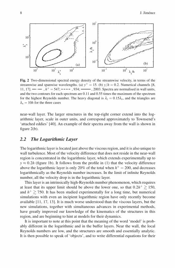
Fig. 2 Two-dimensional spectral energy density of the streamwise velocity, in terms of thestreamwise and spanwise wavelengths. (a) y+ = 15. (b) y/h = 0.2. Numerical channels [8,11, 17]. , h+ = 547; , 934; , 2003. Spectra are normalised in wall units,and the two contours for each spectrum are 0.11 and 0.55 times the maximum of the spectrumfor the highest Reynolds number. The heavy diagonal is λz = 0.15λx, and the triangles areλx = 10h for the three cases
near-wall layer. The larger structures in the top-right corner extend into the log-arithmic layer, scale in outer units, and correspond approximately to Townsend’s‘attached eddies’ [40]. An example of their spectra away from the wall is shown infigure 2(b).
2.2 The Logarithmic Layer
The logarithmic layer is located just above the viscous region, and it is also unique towall turbulence. Most of the velocity difference that does not reside in the near-wallregion is concentrated in the logarithmic layer, which extends experimentally up toy ≈ 0.2h (figure 1b). It follows from the profile in (1) that the velocity differenceabove the logarithmic layer is only 20% of the total when h+ = 200, and decreaseslogarithmically as the Reynolds number increases. In the limit of infinite Reynoldsnumber, all the velocity drop is in the logarithmic layer.
This layer is an intrinsically high-Reynolds number phenomenon, which requiresat least that its upper limit should be above the lower one, so that 0.2h+ � 150,and h+ � 750. It has been studied experimentally for a long time, but numericalsimulations with even an incipient logarithmic region have only recently becomeavailable [11, 17, 13]. It is much worse understood than the viscous layers, but thenew simulations, together with simultaneous advances in experimental methods,have greatly improved our knowledge of the kinematics of the structures in thisregion, and are beginning to hint at models for their dynamics.
It is important to note at this point that the meaning of the word ‘model’ is prob-ably different in the logarithmic and in the buffer layers. Near the wall, the localReynolds numbers are low, and the structures are smooth and essentially analytic.It is then possible to speak of ‘objects’, and to write differential equations for their

Inner-Outer Interactions in Wall-Bounded Turbulence 9
behaviour. Above the buffer layer both things are harder to do. Since the definitionof the outer layer includes y+ � 1, its largest structures have high internal Reynoldsnumbers, and are turbulent themselves. There is presumably a cascade connect-ing those energy-containing structures with the dissipative scales, and their velocityfields can be expected to have nontrivial algebraic spectra and non-smooth geome-tries that can only be described statistically. They are ‘eddies’, rather than ‘vortices’,because turbulent vorticity always resides at the viscous Kolmogorov lengthscale η ,separated from the energy-containing eddies by a scale ratio O(y+3/4).
While the models for the buffer layer are in the realm of direct numerical sim-ulations (DNS), the outer layers are the domain of large-eddy simulations (LES).This of course does not mean that the logarithmic layer can not be DNSed, and itis almost certain that more direct simulations will be required before this part ofthe flow is understood, but we can probably only expect simple models for partialaspects of the structures involved, rather than full ones including all the flow scales.
The first new information provided by the numerics on the logarithmic layer wasspectral. It had been found experimentally that there are very large scales in theouter regions of turbulent boundary layers [19, 27], and DNS provided informa-tion about their two-dimensional spectra, and about their wall-normal correlations[8, 11]. The longest scales are associated with the streamwise velocity component.Its spectral density in the logarithmic layer has an elongated shape along the lineλ 2
z = yλx, while the two other velocity components are more isotropic. When three-dimensional flow fields became available, it was found that there is a self-similarhierarchy of compact ejections extending from the outer flow into the buffer layer,within which the coarse-grained dissipation is more intense than elsewhere [12].They correspond to the isotropic spectra of the wall-normal velocity. When the flowis conditionally averaged around them, they are associated with long, conical, low-velocity regions in the logarithmic layer [12], whose intersection with a y-plane isparabolic, explaining the quadratic behaviour of the spectrum of u. These structuresare not only statistical constructs. Individual cones are observed as low-momentum‘ramps’ in streamwise sections of instantaneous flow fields [29].
When the cones reach heights of the order of the flow thickness, they stop grow-ing, and become cylindrical ‘streaks’ spanning the distance from the central planeto the wall [8, 11], similar to those of the sublayer, but with spanwise scales of2− 3h. They are fully turbulent objects. Neither in simulations nor in experimentsin channels or pipes has it been possible to determine the maximum length of those‘global modes’, which appear in any case to be longer than 25h [11, 18]. There ishowever some evidence that they may be shorter in boundary layers. The overallarrangement of the ejections and cones is reminiscent of the association of vorticesand streaks in the buffer layer, but at a much larger scale. Their near-wall footprintsare seen in the spectra of the buffer layer as the ‘tails’ in figure 2, and account [17]for the experimentally-observed Reynolds number dependence of the intensity ofthe near-wall velocity fluctuations [7].
Since we saw above that the sublayer streaks originate from the advection of themean shear by cross-stream perturbations, which is a linear process, there is somehope that a linear model could also capture the formation of the outer-layer streaks.

10 J. Jimenez
The mean velocity profile of turbulent channels is linearly stable [34], but it hasbeen known for some time that even stable flows can lead to large transient energyamplifications, because the evolution operator of the linearised Navier–Stokes equa-tions is not self-adjoint [15, 4]. Simple linearised analysis of a uniform shear showsthat the long-time asymptotic state of any localised perturbation is a u-streak, butit provides no wavelength-selection mechanism. When the analysis is repeated fornontrivial profiles, such as laminar or turbulent channels, the flow thickness providesa lengthscale and a wall-normal modal structure. The key modelling assumption toobtain structures mimicking the turbulent eddies of the logarithmic and outer re-gions appears to be the use of a y-dependent eddy viscosity similar to that requiredto maintain the experimental mean profile [33, 9]. Note that this implies that theresulting model applies to averaged eddies, rather than to individual structures. Itturns out that there are two sets of wavelengths for which the total energy is mostamplified, with eigenfunctions peaking at the two locations where the viscosity doesnot depend on y. Near the wall, where the viscosity is mostly molecular, they havespanwise wavelengths and eigenfunctions similar to the observed sublayer streaks.Near the central plane, where νT ≈ uτh is also roughly uniform, they are large-scalestreaks with spanwise wavelengths of the order of the observed 3h, and wall-normaleigenfunctions that agree well with the dominant proper orthogonal decompositioneigenmodes of the streamwise velocity at those wavelengths.
3 The Direction of Causality
We know less about how the ejections are created, but linear analysis also givessome information on them. In the same way as the linear effect of transverse per-turbations is to create transient u-streaks, any perturbation of u that is not infinitelylong transfers energy into the transverse velocity components. The same transient-growth analysis giving the large-scale streaks contains nontrivial amplifications forv and w, which could in principle feed a linear cycle in which v ejections createstreaks by extracting energy from the mean shear, while the streaks in turn createejections. Unfortunately the wavelengths of both processes are different, which iswhy the profile is linearly stable. The most amplified u-structures are streaks elon-gated along x, while the most amplified v and w are roughly isotropic in the wall-parallel plane. This agrees with the spectral evidence, but means that nonlinearity isrequired to match the wavelengths, and to close the cycle. It is however easy to visu-alise a process by which an ejection creates a strong streak, whose enveloping shearlayer becomes unstable and creates new, shorter ejections. In fact, we have seen thatcompact ejections can be identified at all scales in the logarithmic and outer layers,both numerically and experimentally, and that they are associated with streaks. Itis known, from the analysis of their relative lengths and lifetimes, that the observedejections cannot be the origin of the full length of the streak to which they are associ-ated, and that some causal link from streaks to ejections is also required [9]. In fact,numerical experiments with ‘minimal’ simulation boxes of the order of the channelwidth, several thousand wall units long and wide, show evidence of an ‘outer’ cycle
Inner-Outer Interactions in Wall-Bounded Turbulence 11
10−1
100
101
10−1
100
101
λx/h
λ z/h
(a)
10−1
100
10110
−2
10−1
100
λz/h
y
/h
(b)
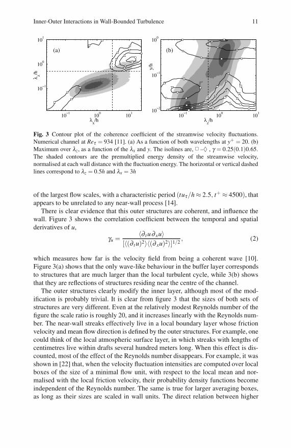
Fig. 3 Contour plot of the coherence coefficient of the streamwise velocity fluctuations.Numerical channel at Reτ = 934 [11]. (a) As a function of both wavelengths at y+ = 20. (b)Maximum over λz, as a function of the λx and y. The isolines are, � –♦ , γ = 0.25(0.1)0.65.The shaded contours are the premultiplied energy density of the streamwise velocity,normalised at each wall distance with the fluctuation energy. The horizontal or vertical dashedlines correspond to λz = 0.5h and λx = 3h
of the largest flow scales, with a characteristic period (tuτ/h≈ 2.5, t+ ≈ 4500), thatappears to be unrelated to any near-wall process [14].
There is clear evidence that this outer structures are coherent, and influence thewall. Figure 3 shows the correlation coefficient between the temporal and spatialderivatives of u,
γu =〈∂ t u∂ xu〉
[〈(∂ t u)2〉〈(∂ xu)2〉]1/2, (2)
which measures how far is the velocity field from being a coherent wave [10].Figure 3(a) shows that the only wave-like behaviour in the buffer layer correspondsto structures that are much larger than the local turbulent cycle, while 3(b) showsthat they are reflections of structures residing near the centre of the channel.
The outer structures clearly modify the inner layer, although most of the mod-ification is probably trivial. It is clear from figure 3 that the sizes of both sets ofstructures are very different. Even at the relatively modest Reynolds number of thefigure the scale ratio is roughly 20, and it increases linearly with the Reynolds num-ber. The near-wall streaks effectively live in a local boundary layer whose frictionvelocity and mean flow direction is defined by the outer structures. For example, onecould think of the local atmospheric surface layer, in which streaks with lengths ofcentimetres live within drafts several hundred meters long. When this effect is dis-counted, most of the effect of the Reynolds number disappears. For example, it wasshown in [22] that, when the velocity fluctuation intensities are computed over localboxes of the size of a minimal flow unit, with respect to the local mean and nor-malised with the local friction velocity, their probability density functions becomeindependent of the Reynolds number. The same is true for larger averaging boxes,as long as their sizes are scaled in wall units. The direct relation between higher

12 J. Jimenez
local friction velocities and higher intensities reverses away from the wall, but eventhere the effect seems to be fairly straightforward. The local friction velocity is justa reflection of the local wall shear, and whenever it is low it is because the meanflow has been lifted away from the wall. This implies that there has to be a highershear somewhere above, since the bulk velocity is constant, and those high-shearregions can be expected to give rise to locally higher production and fluctuation in-tensities. This can be shown to be true, and the correlation coefficient between localfluctuation intensities and local shear is positive, both at the wall and away from it.
The scenario just described is mostly derived from simulations, and from thelinear analysis of the averaged equations of motion. A different scenario has beenproposed from the observation of experimental flow fields. In it, the basic objectis a hairpin vortex growing from the wall, whose induced velocity creates the lowmomentum ramps mentioned above [1]. In that model, which was motivated by thebehaviour of hairpin vortices in the numerical simulation of a particular laminarvelocity profile [43], the hairpins regenerate each other, creating vortex packets thatare responsible for the very long observed streaks [5]. While the two models lookvery different at first sight, they can probably be reconciled to a certain extent, withvortex packets corresponding to the instabilities of the shear layer around the streak.
The main formal difference between the two models is their respective empha-sis on vortices and eddies, although that might be largely a matter of notation. Amore serious difference is the treatment of the effect of the wall. The ‘numerical’model emphasises the effect of the local velocity shear rather than the presence ofthe wall, and a top-down flow of causality. The ‘experimental’ one appears to re-quire the formation of the hairpins in the buffer region, and bottom-up causality.That could again be a matter of notation, but it is more likely due to the reliance ofthe experimental model on laminar numerical simulations, using molecular viscos-ity [43]. There is little question that large structures in turbulence feel the effect ofsmaller ones [33]. While the modelling of this randomising effect as a simple eddyviscosity can be criticised, it should be much closer to reality than the much weakermolecular dissipation of a laminar environment. When the linear evolution of aninitially compact ejection is analysed using the eddy viscosity mentioned above,the structures created near the wall do not grow very much, and most ejectionsobserved at a given wall distance have to be created ‘locally’ [12]. Indeed, numeri-cal experiments in which the viscous wall cycle is artificially removed, have outer-flow ejections and streaks that are essentially identical to those above smooth walls[13, 30]. Experimentally, this is equivalent to the classical observation that the outerlayers in turbulent boundary layers are independent of wall roughness [20].
In summary, there is evidence for at least two regeneration cycles in wall-bounded turbulence, broadly similar, but acting in the buffer and outer layers re-spectively. While the former creates the strongest fluctuations, the latter spans thewhole boundary layer, and contains most of the energy. There is clear evidence forthe effect of the outer cycle on the inner one, mostly as a modulation of its intensity.Essentially, the inner cycle ‘lives’ in the local boundary layers of the outer scales.There is also evidence of the triggering of the outer cycle by the inner one, althoughlimited up to now to relatively low Reynolds numbers which leave open the question
Inner-Outer Interactions in Wall-Bounded Turbulence 13
of whether that interaction would survives as the range of scales involved gets reallylarge. Although it would be strange if absolutely no inner-outer interaction exists,the nature of the trigger is not well understood, and contradicts the evidence thatessentially similar outer regions coexist with very different inner ones, such as overrough walls.
Acknowledgements. The preparation of this paper was supported in part by the CICYTgrant TRA2006–08226. I am deeply indebted to J.C. del Alamo, O. Flores, S. Hoyas, G.Kawahara and M.P. Simens for providing most of the data on which this discussion is based.
References
1. Adrian, R.J., Meinhart, C.D., Tomkins, C.D.: Vortex organization in the outer region ofthe turbulent boundary layer. J. Fluid Mech. 422, 1–54 (2000)
2. Bakewell, H.P., Lumley, J.L.: Viscous sublayer and adjacent wall region in turbulent pipeflow. Phys. Fluids 10, 1880–1889 (1967)
3. Brown, G.L., Roshko, A.: On the density effects and large structure in turbulent mixinglayers. J. Fluid Mech. 64, 775–816 (1974)
4. Butler, K.M., Farrell, B.F.: Three-dimensional optimal perturbations in viscous shearflow. Phys. Fluids A 4, 1637–1650 (1992)
5. Christensen, K.T., Adrian, R.J.: Statistical evidence of hairpin vortex packets in wallturbulence. J. Fluid Mech. 431, 433–443 (2001)
6. Darcy, H.: Recherches experimentales relatives au mouvement de l’eau dans les tuyeaux.Mem. Savants Etrang. Acad. Sci. Paris 17, 1–268 (1854)
7. de Graaff, D.B., Eaton, J.K.: Reynolds number scaling of the flat-plate turbulent bound-ary layer. J. Fluid Mech. 422, 319–346 (2000)
8. del Alamo, J.C., Jimenez, J.: Spectra of very large anisotropic scales in turbulent chan-nels. Phys. Fluids 15, L41–L44 (2003)
9. del Alamo, J.C., Jimenez, J.: Linear energy amplification in turbulent channels. J. FluidMech. 559, 205–213 (2006)
10. del Alamo, J.C., Jimenez, J.: Estimation of turbulent convection velocities and correc-tions to taylor’s approximation. J. Fluid Mech. (2009) (submitted)
11. del Alamo, J.C., Jimenez, J., Zandonade, P., Moser, R.D.: Scaling of the energy spectraof turbulent channels. J. Fluid Mech. 500, 135–144 (2004)
12. del Alamo, J.C., Jimenez, J., Zandonade, P., Moser, R.D.: Self-similar vortex clusters inthe logarithmic region. J. Fluid Mech. 561, 329–358 (2006)
13. Flores, O., Jimenez, J.: Effect of wall-boundary disturbances on turbulent channel flows.J. Fluid Mech. 566, 357–376 (2006)
14. Flores, O., Jimenez, J.: The minimal logarithmic region. In: Proc. Div. Fluid Dyn.,pp. AE–04. Am. Phys. Soc. (2007)
15. Gustavsson, L.H.: Energy growth of three-dimensional disturbances in plane Poiseuilleflow. J. Fluid Mech. 224, 241–260 (1991)
16. Hagen, G.H.L.: Uber den Bewegung des Wassers in engen cylindrischen Rohren.Poggendorfs Ann. Physik Chemie 46, 423–442 (1839)
17. Hoyas, S., Jimenez, J.: Scaling of the velocity fluctuations in turbulent channels up toReτ = 2003. Phys. Fluids 18, 011702 (2006)
18. Hutchins, N., Marusic, I.: Evidence of very long meandering features in the logarithmicregion of turbulent boundary layers. J. Fluid Mech. 579, 467–477 (2007)

14 J. Jimenez
19. Jimenez, J.: The largest scales of turbulence. In: CTR Ann. Res. Briefs, pp. 137–154.Stanford Univ., Stanford (1998)
20. Jimenez, J.: Turbulent flows over rough walls. Ann. Rev. Fluid Mech. 36, 173–196 (2004)21. Jimenez, J., del Alamo, J.C., Flores, O.: The large-scale dynamics of near-wall turbu-
lence. J. Fluid Mech. 505, 179–199 (2004)22. Jimenez, J., Kawahara, G., Simens, M.P., Nagata, M., Shiba, M.: Characterization of
near-wall turbulence in terms of equilibrium and ‘bursting’ solutions. Phys. Fluids 17,015105 (2005)
23. Jimenez, J., Moin, P.: The minimal flow unit in near-wall turbulence. J. Fluid Mech. 225,221–240 (1991)
24. Jimenez, J., Pinelli, A.: The autonomous cycle of near wall turbulence. J. FluidMech. 389, 335–359 (1999)
25. Jimenez, J., Simens, M.P.: Low-dimensional dynamics in a turbulent wall flow. J. FluidMech. 435, 81–91 (2001)
26. Kim, H.T., Kline, S.J., Reynolds, W.C.: The production of turbulence near a smooth wallin a turbulent boundary layer. J. Fluid Mech. 50, 133–160 (1971)
27. Kim, K.C., Adrian, R.J.: Very large-scale motion in the outer layer. Phys. Fluids 11,417–422 (1999)
28. Kolmogorov, A.N.: The local structure of turbulence in incompressible viscous fluids avery large Reynolds numbers. Dokl. Akad. Nauk. SSSR 30, 301–305 (1941); Reprintedin Proc. R. Soc. London. A 434, 9–13 (1991)
29. Meinhart, C.D., Adrian, R.J.: On the existence of uniform momentum zones in a turbu-lent boundary layer. Phys. Fluids 7, 694–696 (1995)
30. Mizuno, Y., Jimenez, J.: Wall turbulence without walls. In: Proc. Div. Fluid Dyn., pp.AA–02. Am. Phys. Soc. (2008)
31. Nagata, M.: Three-dimensional finite-amplitude solutions in plane Couette flow:bifurcation from infinity. J. Fluid Mech. 217, 519–527 (1990)
32. Osterlund, J.M., Johansson, A.V., Nagib, H.M., Hites, M.: A note on the overlap regionin turbulent boundary layers. Phys. Fluids 12, 1–4 (2000)
33. Reynolds, W.C., Hussain, A.K.M.F.: The mechanics of an organized wave in turbu-lent shear flow. Part 3. Theoretical models and comparisons with experiments. J. FluidMech. 54, 263–288 (1972)
34. Reynolds, W.C., Tiederman, W.G.: Stability of turbulent channel flow, with applicationto Malkus’ theory. J. Fluid Mech. 27, 253–272 (1967)
35. Richardson, L.F.: The supply of energy from and to atmospheric eddies. Proc. Roy. Soc.A 97, 354–373 (1920)
36. Robinson, S.K.: Coherent motions in the turbulent boundary layer. Ann. Rev. FluidMech. 23, 601–639 (1991)
37. Smith, C.R., Metzler, S.P.: The characteristics of low speed streaks in the near wall regionof a turbulent boundary layer. J. Fluid Mech. 129, 27–54 (1983)
38. Swearingen, J.D., Blackwelder, R.F.: The growth and breakdown of streamwise vorticesin the presence of a wall. J. Fluid Mech. 182, 255–290 (1987)
39. Tennekes, H., Lumley, J.L.: A first course in turbulence. MIT Press, Cambridge (1972)40. Townsend, A.A.: The structure of turbulent shear flow, 2nd edn. Cambridge U. Press,
Cambridge (1976)41. Waleffe, F.: Three-dimensional coherent states in plane shear flows. Phys. Rev. Lett. 81,
4140–4143 (1998)42. Waleffe, F.: Homotopy of exact coherent structures in plane shear flows. Phys. Fluids 15,
1517–1534 (2003)43. Zhou, J., Adrian, R.J., Balachandar, S., Kendall, T.M.: Mechanisms for generating
coherent packets of hairpin vortices in channel flow. J. Fluid Mech. 387, 353–396 (1999)

Turbulence Interaction with AtmosphericPhysical Processes
Chin-Hoh Moeng and Jeffrey Weil
Abstract. This article reviews the planetary-boundary-layer (PBL) turbulence andits interactions with atmospheric processes. We show three examples: turbulenceresponse to surface heating and cooling over lands, effects of ocean waves, and in-teractions with radiation and cloud microphysics. We also show how computationalfluid dynamics methods are used to gain fundamental understanding of these inter-actions mostly under idealized environments. For certain practical applications inwhich idealized conditions may not apply, a brute-force method may be needed toexplicitly simulate the turbulence interaction. One way is to nest a large-eddy sim-ulation domain inside a weather forecast model, and to allow for turbulence feed-back to other physical processes. This numerical method sounds straightforwardbut poses two major problems. We suggest a systematic approach to examine theproblems.
1 Introduction
Turbulence is a difficult scientific problem because of its highly nonlinear nature.Turbulence poses an even bigger challenge when it interacts with atmospheric phys-ical processes such as the diurnal heating/cooling cycle, ocean waves, clouds, andweather events. There are a variety of turbulence regimes in the atmosphere, dif-fering in scales, characteristics, and the sources of turbulent kinetic energy (TKE).For example, geostrophic turbulence, which results from nonlinear advection, theEarth’s rotation and temperature stratification, consists of ”pancake vortices” that
Chin-Hoh MoengNational center for Atmospheric Research, PO Box 3000, Boulder, CO, 80307-3000, USAe-mail: [email protected]
Jeffrey WeilCooperative Institute for Research in Environmental Sciences, University of Colorado,Boulder, CO 80309e-mail: [email protected]
M. Deville, T.-H. Le, and P. Sagaut (Eds.): Turbulence and Interactions, NNFM 110, pp. 15–24.springerlink.com c© Springer-Verlag Berlin Heidelberg 2010

16 C.-H. Moeng and J. Weil
bear more resemblance to two-dimensional turbulence than three-dimensional (3D)turbulence. Other atmospheric turbulence regimes are more 3D in nature and muchsmaller in scale, including clear-air turbulence (due to wind shear near, e.g., theupper-level jet streams), turbulence inside deep clouds or storms, and turbulence inthe planetary boundary layer (PBL).
In this paper, we will focus only on turbulence in the PBL. The PBL is a distinctturbulent layer adjacent to the Earth’s surface. It is a layer that directly feels the im-pact of the Earth’s surface conditions such as roughness, surface heating/cooling,etc. By definition, the PBL is always turbulent and its turbulent motion is al-ways three-dimensional and time evolving. The PBL depth varies depending onthe sources and sinks of its TKE. On a calm night, when the wind is weak and thesurface is colder than the air (negative buoyancy force), the PBL may become veryshallow or even collapse.
The PBL is an effective medium for transporting and diffusing heat, moistureand chemical species. On a bad pollution day, one can clearly see the smog layer,particularly when it is capped by a strong temperature inversion. Because the majorsources of water, heat and biogeochemical species reside on the Earth’s surface, thePBL plays a crucial role in the energy, water, and biogeochemical cycles on Earth.Every weather or climate model requires a turbulence scheme to represent the effectof the PBL turbulence.
PBL turbulence differs from that of laboratory turbulence in some major ways.First the Reynolds number of turbulence in the PBL is extremely high, on the or-der of 109. The PBL turbulence covers a wide range of scales from millimeters tokilometers with a velocity scale on the order of few ms−1. The Reynolds numberis so high that we consider it infinite. Therefore, the molecular viscosity and diffu-sivity terms are omitted in the governing equations of atmospheric models, includ-ing LESs (Large Eddy Simulations). Close to the Earth’s surface, the viscous layer(order of centimeters) is too thin to resolve in any atmospheric model; the first gridlayer often resides in the inertial, logarithmic layer.
Second, the PBL turbulence is almost always affected by buoyancy or temper-ature stratification, be it positive or negative. There is seldom a purely neutral,shear-driven PBL outdoors.
Another major difference is the entraining top of the PBL. Unlike wind tunnelsbounded by two walls, one side of the PBL is a free entraining surface. The entrain-ing interface divides the turbulent air (below) from the non-turbulent air (above).How PBL turbulence controls entrainment is still poorly understood. Entrainment,which is not a major topic for traditional turbulence research, is one of the mostdifficult–and emphasized—topics in the PBL research.
2 PBL Turbulence and Its Interactions
Turbulence in the PBL is never isotropic and homogeneous due to interactions withthe surface below, the free (non-turbulent) atmosphere above, radiation, or clouds.These interactions significantly change the behavior of energy-containing eddies
Turbulence Interaction with Atmospheric Physical Processes 17
(i.e., eddies larger than tens or hundreds of meters), and these variations make itimpossible to study or quantify the PBL turbulence with a universal scaling law orturbulence scheme. Therfore, the PBL is typically classified into several regimes ac-cording to its interactions or meteorological conditions. In this article we will reviewsome turbulence interactions, and show how computational fluid dynamics methods,such as DNS (Direct Numerical Simulation) and LES (Large Eddy Simulation), areused to study these interactions.
There are two kinds of interactions depending on the time (or spatial) scale of thephysical process that interacts with the turbulence. The turbulence eddy-turnovertime in the PBL is on the order of several mimutes to several tens of minutes de-pending on the PBL regimes. If the time scale of the physical process is much longerthan that of the turbulence eddy-turnover time scale, turbulence can attain equilibrimwith the physical process before the process changes. This interaction establishes astatistically quasi-steady turbulence regime with a given process (or meteorologicalcondition). We will call this an interaction of first kind.
The second kind of interaction is when the time (or spatial) scale of the physicalprocess is similar to or even shorter than the turbulence scale. Interaction takes placeon a time scale where both the turbulence and the process keep adjusting to eachother. Unless otherwise specified, the ”interaction” mentioned in this article belongsto the second kind.
2.1 Interaction with Land Processes and Diurnal Cycle
The diurnal cycle of the PBL is a result of the first kind of interaction with land.When the sun heats the ground, the surface buoyancy flux becomes positive andconvectively drives turbulence in the PBL. This PBL regime is classified as theconvective PBL (CBL) or the unstable PBL. The intensity of convectively driventurbulence is often very strong so that all conserved variables such as potential tem-perature, water vapor mixing ratio (no cloud cases) or air pollutants are well mixedin the CBL. The transport is carried mostly by large turbulent thermals on the size ofthe CBL depth (which is on the order of 1 kilometer), and hence is very efficient andnon-local. These thermals carry heat or moisture from the ground to the top of theCBL within just a few minutes. In the CBL, species originating near the surface candiffuse upwards faster than those from elevated sources diffuse downward, knownas asymmetric transport. The non-local and asymmetric transport properties in theCBL are quite distinct from those of shear-driven turbulence.
After sunset, the ground becomes colder than the air, the buoyancy term in theTKE budget becomes negative, and the PBL decreases abruptly. Shear becomes theonly source of TKE competing with the negative buoyancy force which consumesturbulence. The turbulence intensity in the stable PBL is therefore much weakerthan that in the CBL.
The term ”very stable PBL” applies to the condition when shear production andbuoyancy consumption of TKE are comparable in magnitude. When buoyancy con-sumption dominates, turbulence becomes very weak and may collapse. Weak orno mixing enhances wind shear locally which in turn overcomes the buoyancy

18 C.-H. Moeng and J. Weil
consumption, and turbulence is re-generated. Turbulence in the very stable PBL isthus intermittent in time and space; its properties, depending strongly on the phys-ical processes with which it interacts, may be too variable to describe statistically(see review by [6]). The intermittency and weak TKE also pose a challenge for LES.
Another turbulence regime over land is canopy turbulence where turbulence fromthe PBL and a vegetation canopy interact. Turbulent downbursts in the PBL injectfresh air into the canopy layer generating coherent eddies inside the canopy, whichaffects the canopy turbulence. At the same time relatively humid air from the tran-spiring vegetation is expelled from the canopy and changes the turbulence above. Wewill not elaborate on this topic, but refer those who are interested to [4, 5, 14, 11].
2.2 Interaction with Ocean Waves
Turbulence on both sides of the ocean [the PBL above and the oceanic boundarylayer (OBL) below] interacts strongly with surface gravity waves. Surface wavesare driven by surface winds, and depending on the wind forcing, waves form withdifferent wavelengths and wave heights, propagate at different speeds, and break—sometimes producing sea spray and bubbles. In turn, waves modify winds in thePBL and induce elongated streamwise vortices (Langmuir circulations) in the OBL,thus changing the turbulence. Studies (e.g., [3]) have suggested that hurricane inten-sity and track are sensitive to the turbulence-wave interaction, which remains poorlyunderstood and under-studied.
At NCAR, we started out by developing a DNS to simulate turbulent flow overidealized water waves [17]. Figure 1 shows a sketch of the DNS domain for a Cou-ette flow over a moving wavy boundary to mimic a shear-driven PBL over a wavyocean. This study shows significant influences of the imposed wave on the turbu-lence statistics; the influence depends on the wave age (c/u∗ where c is the wavephase speed and u∗ is the friction velocity) and the wave slope (aκ where a is thewave amplitude and κ the wave number). Figure 2 displays the wave effect on mo-mentum transport, showing that waves moving slower than a certain value of c/u∗generate a more negative momentum flux compared to the flat surface case, whilefast moving waves generate the opposite effect. Very close to the surface all movingwaves lead to a more negative momentum flux due to the wave-correlated flux.
The above DNS has been extended to LES to investigate the effects of wavebreaking and Langmuir circulations on the OBL ([18]) and the effects of mov-ing waves on the PBL ([19]). This LES code is now being extended to includemore realistic waves with multiple wavelengths (personal communication withPeter Sullivan).
The above studies prescribe the wavy surface and hence provide only a one-way interaction of waves with turbulence. A future challenge is to allow for thewavy surface to respond to the turbulence. This two-way interaction study requiresbetter understanding of how waves respond to turbulence, which is lacking, and anumerical technique that provides a time-varying surface coordinate.

Turbulence Interaction with Atmospheric Physical Processes 19
Fig. 1 Sketch of three-dimensional Couette flow drivn by U0 over a moving wavy surface,from Sullivan et al (2000)
Fig. 2 Profiles of the vertical momentum flux for various c/u∗: (a) < uw > /u2∗, and (b)(< uw > − < uw > f lat )/u2∗, from Sullivan et al (2000)

20 C.-H. Moeng and J. Weil
2.3 Interaction with Radiation and Cloud Microphysics
When air inside the PBL becomes saturated, it forms a layer of cloud in the PBL (orfog if the near-surface air is also saturated). An example is the stratocumulus-toppedPBL (STBL) regime over the east coast of major continents during the Northern-Hemisphere summer season. This cloud sheet reflects much more sunlight backto space than the ocean does, while it emits about the same amount of longwaveradiation as the ocean. As a result, the STBL acts to reduce the solar energy into theEarth system. [12] pointed out that a mere 4% increase in the areal coverage of thiscloud regime could produce a 2-3 K decrease of the global mean temperature, whichis enough to compensate for the global warming due to a doubling of the carbondioxide. That is why this cloud regime has brought attention to the geoengineeringcommunity (e.g., [13]).
The cloud amount of the STBL depends strongly on the interactions amongturbulence, radiation and cloud microphysics ([7, 8])—in a time shorter than theeddy turnover time. This PBL regime is unique in that turbulence is driven mainlyby longwave radiative cooling at the cloud top. (Longwave radiative cooling atcloud top occurs because cloudy air emits more longwave radiation than non-cloudy air does, which produces a sharp radiative flux jump right at the cloud top.)Cooling-from-above can generate a positive buoyancy forcing like heating-from-below. However, this cooling occurs at a free interface where the entrainment oc-curring there greatly complicates the problem. Entrainment can warm and cool theair near the cloud top at the same time. When the inversion air is entrained andmixes with the cloudy air, the temperature of the mixture can increase solely bymixing, but it can also decrease due to evaporative cooling of cloud droplets. Thenet result of these two competing effects depends on the temperature and moisturegradients across the STBL top, and this net result can significantly modify the buoy-ancy production for the TKE. So far we cannot represent the STBL regime properlyin climate models because we do not understand quantatively how these interactionschange the cloud amount and turbulent intensity.
Many research groups worldwide have been studying this PBL regime throughfield measurements (e.g., [12, 15]) and LESs. To see if LES is capable of simulatingthis complicated PBL regime, ten groups of LES researchers performed an inter-comparison study of the STBL regime in the mid-1990s ([10]); the result showeda wide spread of the predicted entrainment rates among the ten LES codes. Thisstudy brought attention to the entrainment-rate issue and motivated several fieldcampaigns ([15]) and idealized LES studies (e.g., [1]), designed specifically for bet-ter understanding of the entrainment processes. However, a more recent intercom-parison study ([16]) suggests that we have gained little improvement in our abilityto simulate the entrainment rate in the STBL. The study suggests that the LES tech-nique may be too sensitive to the SGS processes near the cloud top to properly rep-resent the complicated interactions among turbulence, entrainment, radiation andcloud microphysics. The problem is amplified in certain environments where theair above the STBL is particularly dry such that the entrained air may destablize

Turbulence Interaction with Atmospheric Physical Processes 21
the cloud layer and cause it to break up. As far as turbulence interaction withatmospheric physical processes is concerned, this PBL regime provides the bestexample of the interaction complexity.
3 Turbulence in Complex, Real-World Environments
Most of the PBL LESs have been limited to idealized physical conditions, e.g.,horizontally uniform or periodic wavy surfaces. Those conditions are ideal for gain-ing fundamental understanding of turbulence interactions without the real-worldcomplexity. However, some practical PBL applications require real-world settings.For example, to select a wind farm site we need to know the local terrain and weathereffects because they can significantly affect the velocity fluctuations at the wind-turbine height. Air pollution is another example where the local terrain and meteo-rological conditions can modify the PBL turbulence and influence the likelihood ofan extreme (high) concentration event.
A brute-force method to study turbulence interactions with real-world physicalprocesses is to explicitly resolve all relevant scales by using a turbulence-resolvinggrid over the whole domain that covers all scales of the physical processes. However,this may become computationally impossible if the largest scale of the physicalprocesses is much larger than the turbulence scale. One way to solve this problemis to nest an LES domain for the region of interest inside a weather forecast model.A typical weather forecast model consists of realistic terrain geometry and realisticmeteorological conditions, but its grid resolution is too coarse to resolve turbulentmotions; it uses a RANS (Reynolds Averaged Navier-Stokes) model to represent thestatistics of PBL turbulence. Thus, a weather model alone is not a proper tool forstudying turbulence interactions.
The idea of nesting an LES inside a weather model is not new. For example, thestudy by [2] nests an LES domain over the southern Swiss Alps in a weather modelto simulate PBL over steep, mountainous terrain. Their approach allows for justone-way (downscaling) interaction where the mesoscale model prediction drivesthe LES flow. However, the effect of the resolved turbulence field from LES doesnot feedback to the mesoscale prediction.
Two-way nesting allows for two-way interactions between turbulence andmesoscale processes. Two-way nesting uses the outer-domain mesoscale flow fieldto provide the flow conditions along the nest boundaries for the inner-domain LES,and at the same time uses the spatially averaged LES flow field to overwrite theouter-domain solution in the overlapped region.
The two-way nesting concept is straightforward, but there are two major issuesthat need to be examined. First is the spin-up issue: inside the outer domain wherea RANS model is used, the resolved flow field there is Reynolds averaged. Thus,the flows along the nest boundaries (from the outer domain) are non-turbulent mo-tions. Non-turbulent inflow takes time to spin up to fully developed turbulence inmodels because of grid discretization. Based on our experience in performing PBL


![Crue, W. (1932 [renewed 1960, 1988]). Ordeal by Cheque ...20By%20Cheque.pdf · Vanity Fair. Cited in Vacca, R. T., & Vacca, J. L. (1999). Content area reading: Literacy and learning](https://img.pdfslide.us/doc/110x75/5ab10cf07f8b9a1d168c15e7/crue-w-1932-renewed-1960-1988-ordeal-by-cheque-20by20chequepdfvanity.jpg)