1 INTRODUCTION

Developments in spatial data handling have beenconsiderable during the past few decades and itseems likely that this will continue. GIS haveintroduced the integration of spatial data fromdifferent kinds of sources, such as remote sensing,statistical databases, and recycled paper maps. Theirfunctionality offers the ability to manipulate,analyse, and visualise the combined data. Their userscan link application-based models to them and tryto find answers to (spatial) questions. The purpose ofmost GIS is to function as decision support systemsin the specific environment of an organisation.

Maps are important tools in this process. Theyare used to visualise spatial data, to reveal andunderstand spatial distributions and relations.However, maps are no longer the final products theyused to be. Maps are now an integral part of theprocess of spatial data handling. The growth of GIShas changed their use, and as such has changed theworld of those involved in cartography and thoseworking with spatial data in general. This is causedby many factors which can be grouped in three maincategories. First, technological developments infields such as databases, computer graphics,

multimedia, and virtual reality have boosted interestin graphics and stimulated sophisticated (spatial)data presentation. From this perspective it appearsthat there are almost no barriers left. Second, user-oriented developments, often as an explicit reactionto technological developments, have stimulatedscientific visualisation and exploratory data analysis(Anselin, Chapter 17). Also, the cartographicdiscipline has reacted to these changes. Newconcepts such as dynamic variables, digitallandscape models, and digital cartographic modelshave been introduced. Map-based multimedia andcartographic animation, as well as the visualisationof quality aspects of spatial data, are core topics incontemporary cartographic research.

Tomorrow’s users of GIS will require a direct andinteractive interface to the geographical and other(multimedia) data. This will allow them to searchspatial patterns, steered by the knowledge of thephenomena and processes being represented by theinterface. One of the reasons for this is the switchfrom a data-poor to a data-rich environment, but itis also because of the intensified link between GISand application-based models. As a result, anincrease in the demand for more advanced andsophisticated visualisation techniques can be seen.

157

11Visualising spatial distributions

M-J KRAAK

Maps are an integral part of the process of spatial data handling. They are used to visualisespatial data, to reveal and understand spatial distributions and relations. Recentdevelopments such as scientific visualisation and exploratory data analysis have had a greatimpact. In contemporary cartography three roles for visualisation can be recognised. First,visualisation may be used to present spatial information where one needs function to createwell-designed maps. Second, visualisation may be used to analyse. Here functions arerequired to access individual map components to extract information, and functions toprocess, manipulate, or summarise that information. Third, visualisation may be used toexplore. Functions are required to allow the user to explore the spatial data visually, forinstance by animation or linked views.

The developments described here have led tocartographers redefining the word ‘visualisation’(Taylor 1994; Wood 1994). In cartography, ‘tovisualise’ used to mean just ‘to make visible’, and assuch incorporated all cartographic products.According to the newly established Commission onVisualisation of the International CartographicAssociation it reflects ‘. . . modern technology thatoffers the opportunity for real-time interactivevisualisation’. The key concepts here are interactionand dynamics.

The main drive behind these changes has been thedevelopment in science and engineering of the fieldknown as ‘visualisation in scientific computing’(ViSC), also known as scientific visualisation.During the last decade this was stimulated by theavailability of advanced hardware and software. Intheir prominent report McCormick et al (1987)describe it as the study of ‘those mechanisms inhumans and computers which allow them in concertto perceive, use and communicate visualinformation’. In GIS, especially when exploringdata, users can work with the highly interactive toolsand techniques from scientific visualisation. DiBiase(1990) was among the first to realise this. Heintroduced a model with two components: ‘privatevisual thinking’ and ‘public visual communication’.Private visual thinking refers to situations whereEarth scientists explore their own data, for example.Cartographers and their well-designed maps providean example of public visual communication. Thefirst can be described as geographical or map-basedscientific visualisation (Fisher et al 1993;MacEachren and Monmonier 1992). In thisinteractive ‘brainstorming’ environment the raw datacan be georeferenced resulting in maps anddiagrams, while other data can result in images andtext. By the publication of two books, Visualizationin geographical information systems (Hearnshaw andUnwin 1994) and Visualization in moderncartography (MacEachren and Taylor 1994) thespatial data handling community clearlydemonstrated their understanding of the impact andimportance of scientific visualisation on theirdiscipline. Both publications address many aspectsof the relationships between the fields ofcartography and GIS on the one hand, and scientificvisualisation on the other. According to Taylor(1994) this trend of visualisation should be seen asan independent development that will have a majorinfluence on cartography. In his view the basic

aspects of cognition (analysis and applications),communication (new display techniques), andformalism (new computer technologies) are linkedby interactive visualisation (Figure 1).

Three roles for visualisation may be recognised:

● First, visualisation may be used to present spatialinformation. The results of spatial analysisoperations can be displayed in well-designedmaps easily understood by a wide audience.Questions such as ‘what is?’, or ‘where is?’, and‘what belongs together?’ can be answered. Thecartographic discipline offers design rules to helpanswer such questions through functions whichcreate proper well-designed maps (Kraak andOrmeling 1996; MacEachren 1994a; Robinsonet al 1994).

● Second, visualisation may be used to analyse, forinstance in order to manipulate known data. In aplanning environment the nature of two separatedatasets can be fully understood, but not theirrelationship. A spatial analysis operation, such as(visual) overlay, combines both datasets todetermine their possible spatial relationship.Questions like ‘what is the best site?’ or ‘what isthe shortest route?’ can be answered. What isrequired are functions to access individual mapcomponents to extract information and functionsto process, manipulate, or summarise thatinformation (Bonham-Carter 1994).

● Third, visualisation may be used to explore, forinstance in order to play with unknown and often

M-J Kraak

158

Fig 1. Cartographic visualisation (Taylor 1994).

cogn

ition

(ana

lysis

and

appl

icatio

ns)

comm

unication

(new display techniques)

visualisation

interaction and dynamics

formalism(new computer technologies)

raw data. In several applications, such as thosedealing with remote sensing data, there areabundant (temporal) data available. Questions like‘what is the nature of the dataset?’, or ‘which ofthose datasets reveal patterns related to the currentproblem studied?’, and ‘what if . . .?’ have to beanswered before the data can actually be used in aspatial analysis operation. Functions are requiredwhich allow the user to explore the spatial datavisually (for instance by animation or by linkedviews – MacEachren 1995; Peterson 1995).

These three strategies can be positioned in the mapuse cube defined by MacEachren (1994b). As shownin Figure 2, the axes of the cube represent the natureof the data (from known to unknown), the audience(from a wide audience to a private person) and theinteractivity (from low to high). The spheresrepresenting the visualisation strategies can bepositioned along the diagonal from the lower leftfront corner (present: low interactivity, known data,and wide audience) to the upper right back corner(explore: high interactivity, unknown data, privateperson). Locating cartographic publications withinthe cube would reveal a concentration in the lowerleft front corner. However, colouring the dots todifferentiate the publications according to their agewould show many recent publications outside thiscorner and along the diagonal.

The functionality needed for these three strategieswill shape this chapter. Each of them requires its ownvisualisation approach, described in turn in the

following three sections. The first section providessome map basics. It will briefly explain cartographicgrammar, its rules and conventions. Depending on thenature of a spatial distribution, it will suggestparticular mapping solutions. This strategy has themost developed tools available to create effectivemaps to communicate the characteristics of spatialdistributions. When discussing the second strategy,visualisations to support analysis, it will bedemonstrated how the map can work in thisenvironment, and how information critical fordecision-making can be visualised. In a dataexploration environment, the third strategy, it is likelythat the user is unfamiliar with the exact nature of thedata. It is obvious that, compared to both otherstrategies, more appropriate visualisation methodswill have to be applied. Specific visual explorationtools in close relation to ‘new’ mapping methods suchas animation and hypermaps (multimedia) will bediscussed. It is this strategy that will benefit mostfrom developments in scientific visualisation.

2 PRESENTING SPATIAL DISTRIBUTIONS

Maps are uniquely powerful tools for the transferof spatial information. Using a map one can locategeographical objects, while the shapes and coloursof its signs and symbols inform us about thecharacteristics of the objects represented. Mapsreveal spatial relations and patterns, and offer theuser insight into the distribution of particularphenomena. Board (1993) defines the map as‘a representation or abstraction of geographicalreality’ and ‘a tool for presenting geographicalinformation in a way that is visual, digital or tactile’.Traditionally cartographers have concentrated mostof their research efforts on enhancing the transfer ofspatial data. This knowledge is very valuable,although some additional new concepts need to beintroduced as illustrated in Figure 3. The traditionalpaper map functioned not only as an analoguedatabase but also as an information transfermedium. Today a clear distinction is made betweenthe database and presentation functions of the map,known respectively as the Digital Landscape Model(DLM) and Digital Cartographic Model (DCM). ADLM can be considered as a model of reality, basedon a selection process. Depending on the purpose ofthe database, particular geographical objects havebeen selected from reality, and are represented in the

Visualising spatial distributions

159

Fig 2. The three visualisation strategies plotted in MacEachren’s(1994) map use cube.

high

low

inte

ract

ion

audience

public privatekn

own

data unkn

own

explore

analyse

present

database by a data structure (see Dowman, Chapter31; Martin, Chapter 6). Multiple DCMs can begenerated from the same landscape model,depending on the output medium or map design. Tovisualise data in the form of a paper map requires adifferent approach to an onscreen visualisation, anda road map for a vehicle navigation system will lookdifferent from a map designed for a casual tourist.Both, however, can be derived from the same DLM.

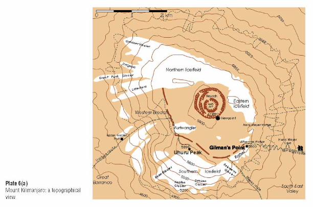
Next in importance to its contents, the usefulnessof a map depends on its scale. For certain GISapplications one needs very detailed large-scalemaps, while others require small-scale maps.Figure 4 shows a small-scale map (on the left) and alarge-scale map. Traditionally maps have beendivided into topographic and thematic types.Topographic maps portray the Earth’s surface asaccurately as possible subject to the limitations ofthe map scale. Topographic maps may include suchfeatures as houses, roads, vegetation, relief,geographical names, and a reference grid. Thematicmaps represent the distribution of a particularphenomenon. In Plate 6 the upper map shows thetopography of the peak of Mount Kilimanjaro inAfrica. The lower thematic map shows the geologyof the same area. As can be noted, the thematic mapcontains information also found in the topographic

map, since to be able to understand the themerepresented one needs to be able to locate it as well.The amount of topographic information requireddepends on the map theme. A geological map willneed more topographic data than a populationdensity map, which normally only needsadministrative boundaries. The digital environmenthas diminished the distinction between the two maptypes. Often both the topographic and the thematicmaps are stored in layers, and the user is able toswitch layers on or off at will.

The design of topographic maps is mostly basedon conventions, of which some date back to thenineteenth century. Examples are representing waterin blue (see MacDevette et al, Chapter 65), forests ingreen, major roads in red, urban areas in black, etc.The design of thematic maps, however, is based on aset of cartographic rules, also called cartographicgrammar. The application of the rules can betranslated in the question ‘how do I say what towhom?’. ‘What’ refers to spatial data and itscharacteristics – for instance whether they are of aqualitative or quantitative nature. ‘Whom’ refers tothe map audience and the purpose of the map – amap for scientists requires a different approach to amap on the same topic aimed at children. ‘How’refers to the design rules themselves.

M-J Kraak

160

Fig 3. Spatial data characteristics: from reality to the map via a digital landscape model and a digital cartographic model.

modelconstruction/

geographic objectselection

select andconstruct

cartographicrepresentation

mediumoutput

reality digitallandscape model

digitalcartographic model

maps

area

geometry,attribute

line

geometry,attribute

point

geometry,attribute

To identify the proper symbology for a map onehas to conduct cartographic data analysis. Theobjective of such analysis is to access thecharacteristics of the data components in order tofind out how they can be visualised. The first stepin the analysis process is to find a commondenominator for all of the data. This commondenominator will then be used as the title of themap. Next the individual component(s) should beaccessed and their nature described. This can bedone by determining the measurement scale, whichcan be nominal, ordinal, interval, or ratio (seeMartin 1996 for a discussion of geographicalcounterparts to these). Qualitative data such asland-use categories are measured on a nominalscale, while quantitative data are measured on theremaining scales. Qualitative data are classifiedaccording to disciplinary convention, such as a soilclassification system, while quantitative data aregrouped together by mathematical method.

When all the information is available the datacomponents should be linked with the graphic sign

system. Bertin (1983) created the base of this system.He distinguished six graphical variables: size, value,texture (grain), colour, orientation, and shape(Plate 7). Together with the location of the symbolsin use these are known as visual variables. Graphicalvariables stimulate a certain perceptual behaviourwith the map user. Shape, orientation, and colourallow differentiation between qualitative data values.Size is a good variable to use when the purpose ofthe map is to show the distribution amounts, whilevalue functions well in mapping data measured onan interval scale. The design process results inthematic maps that are instantly understandable(for example newspaper maps and simple maps suchas the one in Figure 5), and maps which may takesome time to study (for example road maps ortopographic maps – Plate 6(a)). A final categoryincludes maps which require additionalinterpretative skills on the part of the user (forexample geological or soil maps – Plate 6(b)).

Figure 6 presents an overview of some possiblethematic maps. They represent different mapping

Visualising spatial distributions

161

Fig 4. A small-scale map of East Africa, and a large-scale map of Stone Town (Zanzibar).

methods, many of which are found in thecartographic component of GIS software. Inaddition to the measurement scale, it is alsoimportant to take into account the distribution ofthe phenomenon, whether continuous ordiscontinuous, whether boundaries are smooth ornot, and whether the data refer to point, line, area,or volume objects. The maps in Figure 6 are orderedin a matrix with the (dis)continuous nature alongone side and qualitative/quantitative nature alongthe other side. From the above it will be clear thateach spatial distribution requires a unique mappingsolution depending on its character (see also ElshawThrall and Thrall, Chapter 23).

However, if all rules are applied mechanically theresult can still be quite sterile and uninteresting.There is an additional need for a design that isappealing as well. Figure 5 provides an example ofgood design. Here information is ordered accordingto importance and is translated into a visualhierarchy. The urban area of Zanzibar Town is thefirst item on the map that will catch the eye of themap user. The map also shows some other importantingredients needed, such as an indication of the mapscale and its orientation. Placement and style of textcan be seen to play a prominent role too. Text can beused to convey information additional to thatrepresented by the symbols alone, and the graphical

font used for the wording of ‘Zanzibar Town’ hasbeen chosen to express its oriental Arabicatmosphere. However, to be effective the text mustbe placed in an appropriate position with respect tothe relevant symbols.

3 VISUAL ANALYSIS OF SPATIALDISTRIBUTIONS

3.1 Introduction

Since one of a GIS’s major functions is to act as adecision support system, it seems logical that themap as such should play a prominent role. With themap in this role one can even speak of visualdecision support. The maps provide a direct andinteractive interface to GIS data. They can be usedas visual indices to the individual objects representedin the map. Based on the map, users will get answersto more complex questions such as ‘whatrelationship exists?’ This ability to work with mapsand to analyse and interpret them correctly is onevery important aspect of GIS use. However, to getthe right answers the user should adhere to propermap use strategies.

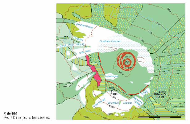
Figure 7 demonstrates that this is not easy at all.The map displayed shows the northern part of theNetherlands. It is a result of a GIS analysis executedby an insurance company which wanted to know ifit would make sense to initiate a regional operation.A first look at the map, which shows the number oftraffic accidents for each municipality, would indeedsuggest so. The eastern region seems to have worsedrivers than the western region. However, a closerlook at the map should make one less sure. First, thegeographical units in the western part are muchlarger than the average units in the east; becauseeach unit has a symbol the map looks much denserin the east. Second, when looking at the legend itcan be seen that the small squares can representfrom 1 to 99 accidents; the map shows some smallsquares representing only one accident, while othersrepresent over 92. The west could therefore still havefar more accidents then the east. The exampleillustrates not only that care is required wheninterpreting maps, but also that access to the map’ssingle objects and the database behind the objects isa necessity. Additional relevant information such asthe number of cars and the length of road should beavailable as well.

M-J Kraak

162

Fig 5. Zanzibar Town: appealing map design by visual hierarchyand the use of fonts.

How can map tools help with the visual analysis ofspatial distributions (Armstrong et al 1992)? Little isknown about how people make decisions on thebasis of map study and analysis. Giffin (1983) foundthat the strategies followed by individuals varywidely in relation to map type and complexity aswell as according to individual characteristics. Fromthe example above, it becomes clear that the userneeds to have access to the appropriate spatial data

in order to solve spatial tasks. Compared to themapping activities in the previous section, the linkbetween map and database (DCM and DLM) aswell as access to the tools to describe andmanipulate the data are of major importance. A keyword here is interaction.

In order to make justifiable decisions based onspatial information, its nature and its quality (orreliability) must be known (Beard and Buttenfield,

Visualising spatial distributions

163

Fig 6. A subdivision of thematic map types, based on the nature of the data (after Kraak andOrmeling 1996).

qualitative quantitative

nominal ordinal/interval/ratio composite

graphicvariables

variation of hue,orientation, form

repetitionvariation of grainsize, grey value

variation of size,segmentation

pointdata

lineardata

a) lines

b) vectors

disc

rete

dat

a

arealdata

regulardistribution

nominal point dot maps proportionalsymbol

point diagram

nominal line symbolmaps

flowline maps line diagram

standardvector maps

graduated vectormaps

vector diagrammaps

R.S. landuse maps regular gridsymbol maps

proportional symbolgrid maps

grid choropleth

areal diagram grid

irregularboundaries

volumedata

surfacedata

chorochromatic mosaicmaps

choropleth areal diagram

stepped statisticalsurface

isoline map filled in isolinemap

volumedata

smooth statisticalsurface

cont

inua

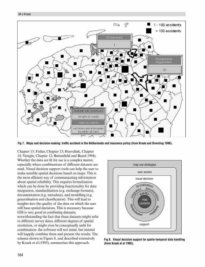
Chapter 15; Fisher, Chapter 13; Heuvelink, Chapter14; Veregin, Chapter 12; Buttenfield and Beard 1994).Whether the data are fit for use is a complex matter,especially where combinations of different datasets areused. Visual decision support tools can help the user tomake sensible spatial decisions based on maps. This isthe most efficient way of communicating informationabout spatial reliability. This requires formalisationwhich can be done by providing functionality for dataintegration, standardisation (e.g. exchange formats),documentation (e.g. metadata), and modelling (e.g.generalisation and classification). This will lead toinsights into the quality of the data on which the userwill base spatial decisions. This is necessary becauseGIS is very good at combining datasets;notwithstanding the fact that these datasets might referto different survey dates, different degrees of spatialresolution, or might even be conceptually unfit forcombination: the software will not mind, but insteadwill happily combine them and present the results. Theschema shown in Figure 8, and described extensivelyby Kraak et al (1995), summarises this approach.

M-J Kraak

164

Fig 7. Maps and decision-making: traffic accident in the Netherlands and insurance policy (from Kraak and Ormeling 1996).

Fig 8. Visual decision support for spatio-temporal data handling(from Kraak et al 1995).

map use strategies

user access

visual decision

mapcontents

support

quality

inte

gration documentation

standardisation modelli

ng

formalisation

While working with spatial data in a GISenvironment one commonly has to deal with‘where?’, ‘what?’, and ‘when?’ queries. In a spatialanalysis operation the queries will result in themanipulation of geometric, attribute, or temporaldata components, separately or in combination.However, just looking at a map that displays thedata already allows an evaluation of how certainphenomena vary in quantity or quality over themapped area. Often one is not just interested in asingle phenomenon but in multiple phenomena. Forsome aspects analytical operations are required, butsometimes a visual comparison will revealinteresting patterns for further study. Spatial,thematic, and temporal comparisons can bedistinguished (Kraak and Ormeling 1996).

3.2 Comparing spatial data’s geometric component

Comparing two areas seems to be relatively easywhile focusing on a single theme – for example,hydrology, relief, settlements, or road networks.However, to make a sensible comparison the mapsunder study should have been compiled according tothe same methods. They should have the same scaleand the same level of generalisation or adhere to thesame classification methods. For instance, if one iscomparing the hydrological patterns in two riverbasins the individual rivers should be represented atthe same level of detail in respect to generalisationand order of branches.

Figure 9 shows a comparison of the islands ofZanzibar and Pemba. They have been isolated fromtheir original location and positioned next to eachother. The coastline, reefs, road network, and villagesare displayed, all derived from the Digital Chart ofthe World. It can be seen that Pemba, the island onthe right, has a typical north–south settlementpattern, while Zanzibar, slightly larger, has a moreevenly spread settlement with a larger urban area onthe west coast (see Openshaw and Alvanides, Chapter18, for a discussion of the analysis of geographicallyaveraged data).

3.3 Comparing the attribute components ofspatial data

If two or more themes related to a particular areaare mapped according to the same method, it ispossible to compare the maps and judge similaritiesor differences. However, not all mapping methods

are easy to compare. Choropleth maps are thesimplest to compare, at least as long as theadministrative units are the same in both maps.Isoline maps can be compared by measuring valuesin each map at the same locations.

Figure 10 compares a chorochromatic map (a soilmap, right) with an isoline map (precipitation, left).At first sight it appears that low precipitationcorresponds with a soil type that dominates theeastern part of the island, and that highprecipitation results in a wider diversity of soils.Those familiar with Earth science in general willknow that there is no necessary link between the twotopics, but the above visual map analysis could be

Visualising spatial distributions

165

Fig 9. Comparing location: Zanzibar (Unguja) and Pemba.

0 30km

Fig 10. Comparing attributes: precipitation and soils.

0 30km

true. It shows that only the expert can do the realanalytical work, but comparing or overlaying twodatasets can be done by anybody – but whether theoperation makes sense remains unanswered.

3.4 Comparing the temporal components ofspatial data

Users of GIS are no longer satisfied with analysis ofsnapshot data but would like to understand andanalyse whole processes. A common goal of this typeof analysis is to identify typical patterns in space-time. Change can be visually represented in a singlemap. Understanding the temporal phenomena froma single map will depend on the cartographic skills ofboth the map maker and map user, since these mapstend to be relatively complex. An alternative is theuse of a series of single maps each representing amoment in time. Comparing these maps will give theuser an idea of change. The number of maps islimited since it is difficult to follow long series ofimages. Another, relatively new alternative is the useof dynamic displays or animation (Kraak andMacEachren 1994). Change in the display over timeprovides a more direct impression of change in thephenomenon represented.

Figure 11 visualises the growth of the populationof Zanzibar. From the maps it becomes clear thatthere is growth, and that growth in the urban districtis faster than in the other parts of the island.

4 VISUAL EXPLORATION OFSPATIAL DISTRIBUTIONS

4.1 Introduction

Keller and Keller (1992) identify three steps in thevisualisation process: first, to identify the visualisationgoal; second, to remove mental roadblocks; and third,to design the display in detail. In cartography the firststep is summarised by the phrase ‘how do I say whatto whom?’, which was addressed in section 2. In thesecond step, the authors suggest removing oneselfsome distance from the discipline in order to reducethe effects of traditional constraints and conventionalwisdom. Why not choose an alternative mappingmethod? For instance, one might use an animationinstead of a set of single maps to display change overtime; show a video of the landscape next to atopographic map; or change the dimension of themap from 2 dimensions to 3 dimensions. New, fresh,creative graphics could be the result, would probablyhave a greater and longer lasting impact thantraditional mapping methods, and might also offerdifferent insight. During the third step, which isparticularly applicable in an exploratory environment,one has to decide between mapping data orvisualising phenomena. An example of the mappingof the amount of rainfall may be used to clarify thisdistinction (Figure 12). Experts exploring rainfallpatterns would like to distinguish between different

M-J Kraak

166

Fig 11. Comparing time: population growth.

0 30km

precipitation classes, by using different colours foreach class, such as blue, red, yellow, and green. Awider television audience might prefer a map showingareas with high and low precipitation. This can berealised using one colour, for instance blue, indifferent tints for all classes. Making dark tintscorrespond with high rainfall and light tints with lowrainfall would result in an instantly understandablemap. When exploring, data visualisation might befavoured; while presenting, phenomena visualisationmay be preferred.

This approach to visualisation requires that aflexible and extensive functionality be available. Thekeywords ‘interaction’ and ‘dynamics’ werementioned before. Compared with the presentationand analytical visualisation strategies these areclearly the extras. However, options to visualise thethird dimension as well as temporal datasets shouldalso be available. When exploring their data, userscan work with the highly interactive tools andtechniques from scientific visualisation. How arethose tools implemented in a geographicalexploratory visualisation environment?

Work is currently underway to develop tools forthis exploratory environment (DiBiase et al 1992;Fisher et al 1993; Kraak 1994; Monmonier 1992;Slocum et al 1994). In 1990 Monmonier introducedthe term‘brushing’, as illustrated in Figure 13. It is

about the direct relationship between the map andother graphics related to the mapped phenomenon,like diagrams and scatter plots. The selection of anobject in the map will automatically highlight thecorresponding elements in the other graphics.Depending on the view in which the object isselected, the options are with geographicalbrushing (clicking in the map), attribute brushing(clicking in the diagram), and temporal brushing(clicking on the time line). Similar experiments onclassification of choropleth maps have been madeby Egbert and Slocum (1992). MacDougall (1992)followed a similar approach, while Haslett et al(1990) developed the Regard package as aninteractive graphic approach to visualisingstatistical data. Other applications are discussed byDiBiase et al (1992), and Anselin (Chapter 17).Dykes (1995) has built a prototype of what he callsa cartographic data visualiser (CDV) which hasmuch exploratory functionality. The systemconsists of a set of linked widgets, such as slidebars, buttons, and labels.

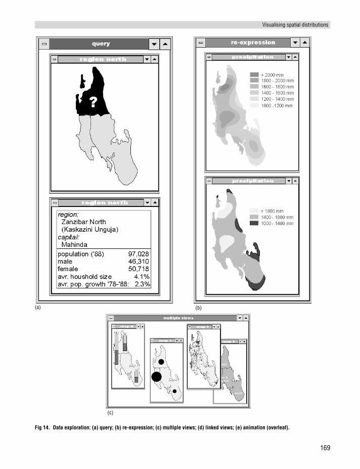
The illustrations in Figure 14 show some of theimportant functions that should be available toexecute an exploratory visualisation strategy. Thefollowing functions are discussed in the worksreferred to above:

Visualising spatial distributions

167

Fig 12. Visualising the classification: phenomena (left) or data (right).

0 25km

● Query: an elementary function, that shouldalways be available whatever the strategy. Theuser can query the map by clicking a symbol,which will activate the database. Electronic atlasesincorporate this functionality (Figure 14(a): seealso Elshaw Thrall and Thrall, Chapter 23).

● Re-expression: this function allows the same data,or part of the data, to be visualised in differentways. A time series of earthquakes could bereordered by the Richter scale instead, which couldreveal interesting spatial patterns; or theclassification method followed could be changedand the grey tints inverted as well – as can be seenin Figure 14(b).

● Multiple views: this approach could be describedas interactive cartography. The same data couldbe displayed according to different mappingmethods. Population statistics could be visualisedas a dot map, a proportional circle map or adiagram map as shown in Figure 14(c).

● Linked views: this option is related toMonmonier’s brushing principle. Selecting a

geographical object in one map will automaticallyhighlight the same object in other views. Forinstance clicking a geographical unit in acartogram would change the colour of the sameunit in a geometrically correct map. In Figure14(d), clicking the diagram showing cloveproduction reveals a photograph of a clove plantand a map with the distribution of cloveplantations in that particular year. This type offunctionality allows one to introduce themultimedia components which will be discussedlater in this section.

● Animation: the dynamic display of (temporal)processes is best done by animation. As will beexplained in the next section interaction is anecessary add-on to animation (Figure 14(e)).

● Dimensionality: to view 3-dimensional spatialdata one should be able to position the map in3-dimensional space with respect to the map’spurpose and the phenomena mapped (seeHutchinson and Gallant, Chapter 19). This meansthat all kinds of interactive geometrictransformation functions to scale, translate, rotate,and zoom should be available, because it may bethat the features of interest are located behindother features in the image (Figure 15).

4.2 Animation

Maps often represent complex processes whichcan be explained expressively by animation. Topresent the structure of a city, for example,animations can be used to show subsequent maplayers which explain the logic of this structure(first relief, followed by hydrography,infrastructure, and land-use, etc.). Animation isalso an excellent way to introduce the temporalcomponent of spatial data, as in the evolution of ariver delta, the history of the Dutch coastline, orthe weather conditions of last week. An interestingexample is ClockWork’s Centennia (previouslyMillennium: ClockWork 1995; http://www.clockwk.com), a historical electronic atlas which presents aninteractive animation of Europe’s boundarychanges between the years 1000 and 1995. Thistype of product can be used to explore or analysethe history of Europe.

The need in the GIS environment to deal withprocesses as a whole, and no longer with single time-slices, also influences visualisation. It is no longer

M-J Kraak

168

Fig 13. Geographic, attribute, and temporal brushing(Monmonier 1990).

Metropolitanpopulation

Per capitaincome ($)

Cablepenetration

Scatterplotbrush

Temporalbrush

Geographicbrush

1985

1973 1989

Visualising spatial distributions

169

Fig 14. Data exploration: (a) query; (b) re-expression; (c) multiple views; (d) linked views; (e) animation (overleaf).

query

(a) (b)

(c)

efficient to visualise models or planning operationsusing static paper maps. However, the onscreen mapdoes offer opportunities to work with moving andblinking symbols, and is very suitable for animation.Such maps provide a strong method of visual

communication, especially as they can incorporatereal data, as well as abstract and conceptual data.Animations not only tell a story or explain a process,but also have the capability to reveal patterns orrelationships which would not be evident if onelooked at individual maps.

Attempts to apply animation to visualise spatialdistributions date from the 1960s (see, for example,Thrower 1961; Tobler 1970) although only non-digital cartoons were possible initially. During the1980s technological developments gave a secondimpulse to cartographic animation (see Moellering1980). A third wave of interest in animation hasdeveloped, driven by interest in GIS (DiBiase et al1992; Langran 1992; Monmonier 1990; Weber andButtenfield 1993). Historic overviews are given byCampbell and Egbert (1990) and Peterson (1995).

The field of (cartographic) animation is about tochange. Peterson (1995) expresses this as ‘whathappens between each frame is more important thenwhat exists on each frame’. This should worrycartographers since their tools were developed mainlyfor the design of static maps. How can we deal withthis new phenomenon? Is it possible to provide theproducers of cartographic animation with sets oftools and rules to create ‘good’ animation, in the form‘If your data are . . ., and your aim is . . ., then usethe variables . . .’? To be able to do so, and to takeadvantage of knowledge of computer graphicsdevelopments and the ‘Hollywood’ scene, the natureand characteristics of cartographic animations haveto be understood. However, the problem is that‘understanding’ animations alone will not be of muchhelp, since the environment where they are used, thepurpose of their use, and the users themselves willgreatly influence ‘performance’.

How can an animation be designed to make surethe viewer indeed understands the trend orphenomenon? The traditional graphic variables, asexplained earlier, are used to represent the spatialdata in each individual frame. Bertin, the first towrite on graphic variables, had a negative approachto dynamic maps. He stated in his work (1967): ‘. . .however, movement only introduces one additionalvariable, it will be dominant, it will distract allattention from the other (graphic) variables’. Recentresearch, however, has demonstrated that this is notthe case. Here we should remember thattechnological opportunities offered at the end of the1960s were limited compared with those of today.Koussoulakou and Kraak (1992) found that theviewer of an animation would not necessarily get a

M-J Kraak

170

Fig 15. Working with the third dimension (from Kraak andOrmeling 1996).

Fig 14. (cont.)

(d)

(e)

better or worse understanding of the contents of theanimation when compared with static maps. DiBiaseet al (1992) found that movement would give thetraditional variable new energy.

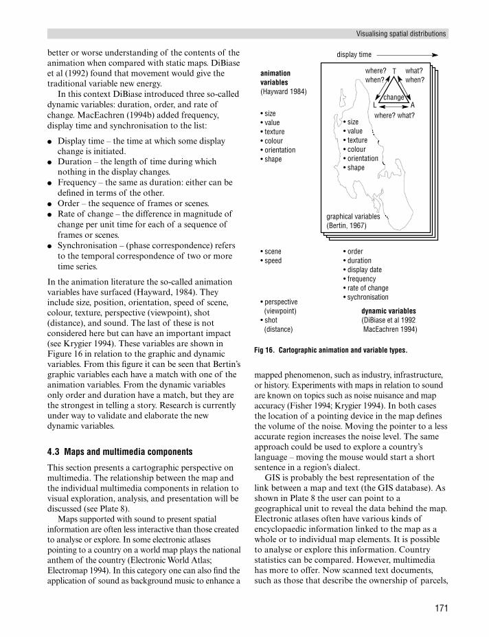
In this context DiBiase introduced three so-calleddynamic variables: duration, order, and rate ofchange. MacEachren (1994b) added frequency,display time and synchronisation to the list:

● Display time – the time at which some displaychange is initiated.

● Duration – the length of time during whichnothing in the display changes.

● Frequency – the same as duration: either can bedefined in terms of the other.

● Order – the sequence of frames or scenes.● Rate of change – the difference in magnitude of

change per unit time for each of a sequence offrames or scenes.

● Synchronisation – (phase correspondence) refersto the temporal correspondence of two or moretime series.

In the animation literature the so-called animationvariables have surfaced (Hayward, 1984). Theyinclude size, position, orientation, speed of scene,colour, texture, perspective (viewpoint), shot(distance), and sound. The last of these is notconsidered here but can have an important impact(see Krygier 1994). These variables are shown inFigure 16 in relation to the graphic and dynamicvariables. From this figure it can be seen that Bertin’sgraphic variables each have a match with one of theanimation variables. From the dynamic variablesonly order and duration have a match, but they arethe strongest in telling a story. Research is currentlyunder way to validate and elaborate the newdynamic variables.

4.3 Maps and multimedia components

This section presents a cartographic perspective onmultimedia. The relationship between the map andthe individual multimedia components in relation tovisual exploration, analysis, and presentation will bediscussed (see Plate 8).

Maps supported with sound to present spatialinformation are often less interactive than those createdto analyse or explore. In some electronic atlasespointing to a country on a world map plays the nationalanthem of the country (Electronic World Atlas;Electromap 1994). In this category one can also find theapplication of sound as background music to enhance a

mapped phenomenon, such as industry, infrastructure,or history. Experiments with maps in relation to soundare known on topics such as noise nuisance and mapaccuracy (Fisher 1994; Krygier 1994). In both casesthe location of a pointing device in the map definesthe volume of the noise. Moving the pointer to a lessaccurate region increases the noise level. The sameapproach could be used to explore a country’slanguage – moving the mouse would start a shortsentence in a region’s dialect.

GIS is probably the best representation of thelink between a map and text (the GIS database). Asshown in Plate 8 the user can point to ageographical unit to reveal the data behind the map.Electronic atlases often have various kinds ofencyclopaedic information linked to the map as awhole or to individual map elements. It is possibleto analyse or explore this information. Countrystatistics can be compared. However, multimediahas more to offer. Now scanned text documents,such as those that describe the ownership of parcels,

Visualising spatial distributions

171

Fig 16. Cartographic animation and variable types.

animationvariables(Hayward 1984)

• size• value• texture• colour• orientation• shape

• scene• speed

• order• duration• display date• frequency• rate of change• sychronisation

• perspective (viewpoint)• shot (distance)

dynamic variables(DiBiase et al 1992 MacEachren 1994)

display time

• size• value• texture• colour• orientation• shape

graphical variables(Bertin, 1967)

T

L Achange

where?when?

what?when?

where? what?

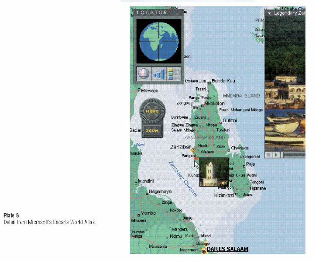
can be included. Text in the format of hypertext canbe used as a lead to other textual information orother multimedia components.

Maps are models of reality. Linking video orphotographs to the map will offer the user adifferent perspective on reality. Topographic mapspresent the landscape, but it is also possible topresent, next to this map, a non-interpreted satelliteimage or aerial photograph to help the user in his orher understanding of the landscape. The analysis ofa geological map can be enhanced by showinglandscape views (video or photographs) fromcharacteristic spots in the area. A real estate agentcould use the map as an index to explore all housesfor sale on company file. Pointing at a specific housewould show a photograph of the house, theconstruction drawings, and a video would startshowing the house’s interior. New opportunities inthe framework are offered by the application ofvirtual reality in GIS.

ReferencesArmstrong M P, Densham P J, Lolonis P, Rushton G 1992

Cartographic displays to support locational decision making.Cartography and Geographic Information Systems 19: 154–64

Bertin J 1983 Semiology of graphics. Madison, University ofWisconsin Press (original in French, 1967)

Board C 1993 Spatial processes. In Kanakubo T (ed.) Theselected main theoretical issues facing cartography: report ofthe ICA Working Group to Define the Main Theoretical Issuesin Cartography. Cologne, International CartographicAssociation: 21–4

Bonham-Carter G F 1994 Geographical information systemsfor geo-scientists: modelling with GIS. New York, PergamonPress

Buttenfield B P, Beard M K 1994 Graphical and geographicalcomponents of data quality. In Hearnshaw H, Unwin D J(eds) Visualisation in geographic information systems.Chichester, John Wiley & Sons: 150–7

Campbell C S, Egbert S L 1990 Animated cartography: thirtyyears of scratching the surface. Cartographica 27: 24–46

ClockWork Software 1995 Centennia. PO Box 148036,Chicago 60614, USA

DiBiase D 1990 Visualization in earth sciences. Earth andMineral Sciences, Bulletin of the College of Earth andMineral Sciences, Pennsylvania State University 59: 13–18

DiBiase D, MacEachren A M, Krygier J B, Reeves C 1992Animation and the role of map design in scientificvisualisation. Cartography and Geographic InformationSystems 19: 201–14

Dykes J 1995 Cartographic visualisation for spatial analysis.Proceedings, Seventeenth International CartographicConference, Barcelona: 1365–70

Egbert S L, Slocum T A 1992 EXPLOREMAP: anexploration system for choropleth maps. Annals of theAssociation of American Geographers 82: 275–88

Fisher P F 1994a Randomization and sound for thevisualization of uncertain spatial information. In HearnshawH, Unwin D J (eds) Visualization in geographic informationsystems. Chichester, John Wiley & Sons: 181–5

Fisher P, Dykes J, Wood J 1993 Map design and visualisation.The Cartographic Journal 30: 136–42

Giffin T L C 1983 Problem-solving on maps – the importanceof user strategies. The Cartographic Journal 20: 101–109

Haslett J, Willis G, Unwin A 1990 SPIDER: an interactivestatistical tool for the analysis of spatially distributed data.International Journal of Geographical Information Systems 4:285–96

Hayward S 1984 Computers for animation. Norwich, PageBros

Hearnshaw H M, Unwin D J (eds) 1994 Visualization ingeographical information systems. Chichester, John Wiley& Sons

Keller P R, Keller M M 1992 Visual cues, practical datavisualization. Piscataway, IEEE Press

Koussoulakou A, Kraak M J 1992 Spatio-temporal maps andcartographic communication. The Cartographic Journal29:101–8

Kraak M J 1994 Interactive modelling environment for 3-Dmaps, functionality and interface issues. In MacEachren AM, Taylor D R F (eds) Visualization in modern cartography.Oxford, Pergamon: 269–86

Kraak M J, MacEachren A M 1994b Visualization of spatialdata’s temporal component. In Waugh T C, Healey R G(eds) Advances in GIS research – Proceedings Fifth SpatialData Handling Conference. London, Taylor and Francis:391–409

Kraak M-J, Ormeling F J 1996 Cartography, visualization ofspatial data. Harrow, Longman

Kraak M-J, Ormeling F J, Müller J-C 1995 GIS-cartography:visual decision support for spatio-temporal data handling.International Journal of Geographical Information Systems 9:637–45

Krygier J 1994 Sound and cartographic visualization. InMacEachren A M, Taylor D R F (eds) Visualization inmodern cartography. Oxford, Pergamon: 149–66

Langran G 1992 Time in geographical information systems.London, Taylor and Francis

MacDougall E B 1992 Exploratory analysis, dynamicstatistical visualization, and geographic information systems.Cartography and Geographic Information Systems 19: 237–46

MacEachren A M 1994a Some truth with maps: a primer ondesign and symbolization. Washington DC, Association ofAmerican Geographers

MacEachren A M 1994b Visualization in modern cartography:setting the agenda. In MacEachren A M, Taylor D R F (eds)Visualization in modern cartography. Oxford, Pergamon: 1–12

M-J Kraak

172

MacEachren A M 1995 How maps work. New York, GuilfordPress

MacEachren A M, Monmonier M 1992 Geographicvisualization: introduction. Cartography and GeographicInformation Systems 19: 197–200

MacEachren A M, Taylor D R F (eds) 1994 Visualization inmodern cartography. Oxford, Pergamon

Martin D J 1996 Geographic information systems:socioeconomic applications. London, Routledge

McCormick B, DeFanti T A, Brown M D 1987 Visualizationin scientific computing. ACM SIGGRAPH ComputerGraphics 21 special issue.

Moellering H 1980 The real-time animation of 3-dimensionalmaps. The American Cartographer 7: 67–75

Monmonier M 1990 Strategies for the visualization ofgeographic time-series data. Cartographica 27: 30–45

Monmonier M 1992 Authoring graphic scripts: experiencesand principles. Cartography and Geographic InformationSystems 19: 247–60

Peterson M P 1995 Interactive and animated cartography.Englewood Cliffs, Prentice-Hall

Robinson A H, Morrison J L, Muehrcke P C, Kimerling A J,Guptill S C 1994 Elements of cartography, 6th edition. NewYork, John Wiley & Sons Inc.

Slocum T A , Egbert S, Weber C, Bishop I, Dungan J,Armstrong M, Ruggles A, Demetrius-Kleanthis D, Rhyne T,Knapp L, Carron J, Okazaki D 1994 Visualization softwaretools. In MacEachren A M, Taylor D R F (eds) Visualizationin modern cartography. Oxford, Pergamon: 91–122

Taylor D R F 1994 Perspectives on visualization and moderncartography. In MacEachren A M, Taylor D R F (eds)Visualization in modern cartography. Oxford, Pergamon: 333–42

Thrower N 1961 Animated cartography in the United States.International Yearbook of Cartography: 20–8

Tobler W R 1970 A computer movie: simulation of populationchange in the Detroit region. Economic Geography 46: 234–40

Weber R, Buttenfield B P 1993 A cartographic animation ofaverage yearly surface temperatures for the 48 contiguousUnited States: 1897–1986. Cartography and GeographicInformation Systems 20: 141–50

Wood M 1994 Visualization in a historical context. InMacEachren A M, Taylor D R F (eds) Visualization inmodern cartography. Oxford, Pergamon: 13–26

Visualising spatial distributions

173