11

Sorting Buffers on HSTs

Harald Räcke

Matthias Englert Matthias Westermann

22

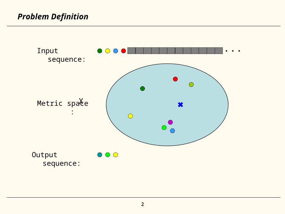
Problem Definition

Input sequence:

Output sequence:

Metric space : X

33

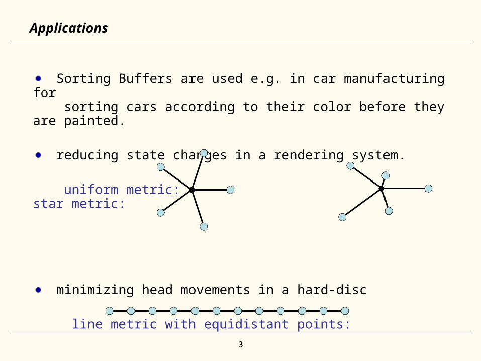
Sorting Buffers are used e.g. in car manufacturing for sorting cars according to their color before they are painted.

reducing state changes in a rendering system.

uniform metric: star metric:

minimizing head movements in a hard-disc

line metric with equidistant points:

Applications

44

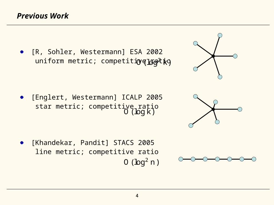
[R, Sohler, Westermann] ESA 2002 uniform metric; competitive ratio

[Englert, Westermann] ICALP 2005 star metric; competitive ratio

[Khandekar, Pandit] STACS 2005 line metric; competitive ratio

Previous Work

O(log2 k)

O(logk)

O(log2 n)

55

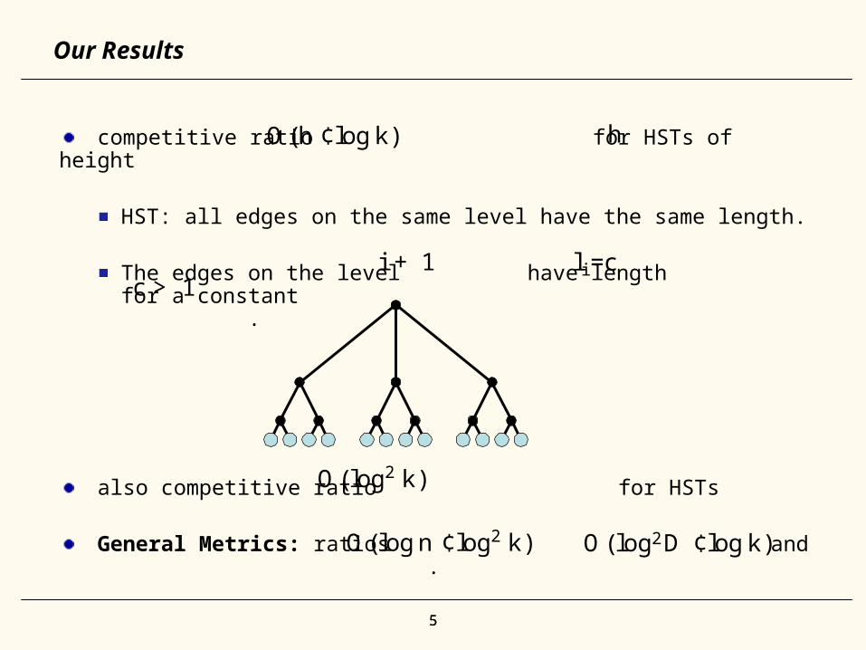
competitive ratio for HSTs of height

HST: all edges on the same level have the same length.

The edges on the level have length for a constant .

also competitive ratio for HSTs

General Metrics: ratios and .

Our Results

h

l i =cc > 1

O(h ¢logk)

i + 1

O(log2D ¢logk)

O(log2 k)

O(logn ¢log2 k)

66

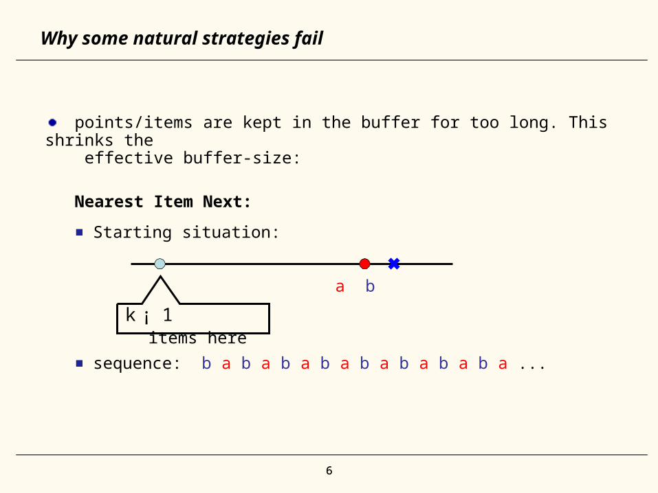
points/items are kept in the buffer for too long. This shrinks the effective buffer-size:

Nearest Item Next:

Starting situation:

sequence: b a b a b a b a b a b a b a b a ...

Why some natural strategies fail

items herek ¡ 1

a b

77

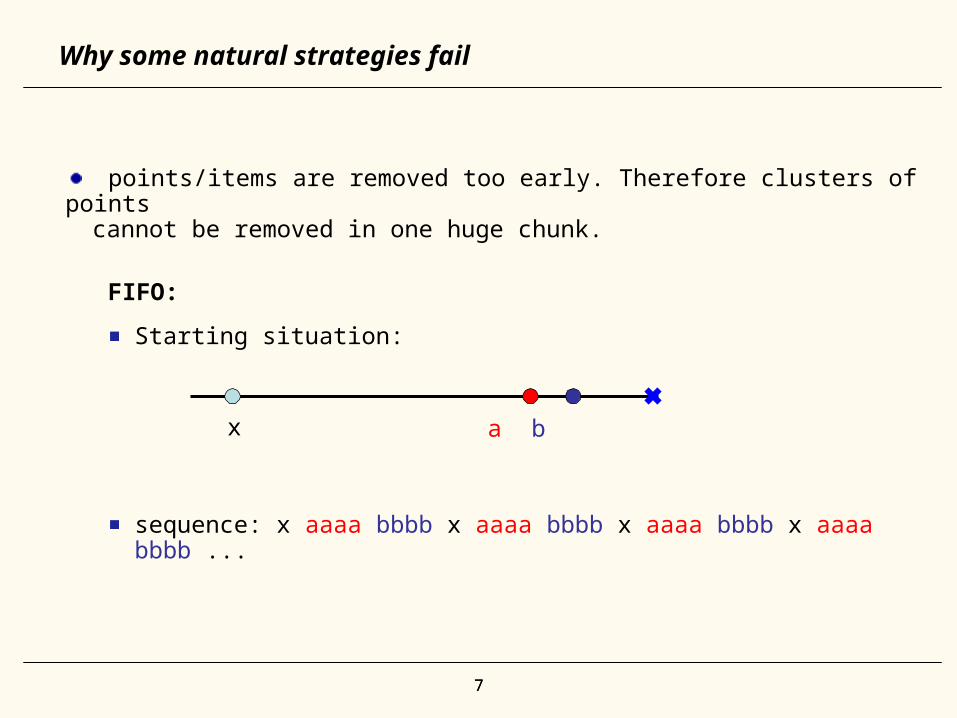
points/items are removed too early. Therefore clusters of pointscannot be removed in one huge chunk.

FIFO:

Starting situation:

sequence: x aaaa bbbb x aaaa bbbb x aaaa bbbb x aaaa bbbb ...

Why some natural strategies fail

a bx

88

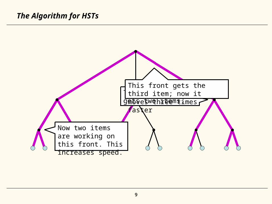
The Algorithm for HSTs

The algorithm is defined by the following continuous process.

Every item in the buffer sends out an agent

In time step an agent places payment on the first yet unpaidedge in direction towards the current ONLINE-position.

When a group of agents arrives at the ONLINE-position, the corresponding items are removed from the buffer and their payment is removed from the edges.

ONLINE moves to the furthest among the just removed items.

t vdt

99

The Algorithm for HSTs

Now two items are working on this front. This increases speed.

This front also gets two items.

This front gets the third item; now it moves three times faster

1010

Observation

The total payment is equal to the ONLINE-cost.

Idea:

fix an optimal algorithm OPT

analyze the payment that is created on an edge between two visits of OPT to this edge

Analysis

1111

Introduce discounts:

Whenever an ONLINE-item creates a unit of payment,an OPT-item creates a discount of on every ancestor

edge.

An ONLINE-item creates a discount of on every ancestor edge, as well.

The total discount that is produced is only half the total payment.

Idea:

analyze the „real payment“ created on an edge (payment-discount) between two consecutive visits of OPT to the edge.

Analysis

vdtvdt=4h

vdt=4h

1212

Amortization: move payment between edges, such that (in the end) for every edge accepted_payment(e) f OPT(e)

– don‘t delete payment

The amortization is done with respect to the actions of the ONLINE, and OPTIMAL algorithm.

Analysis

· ¢

1313

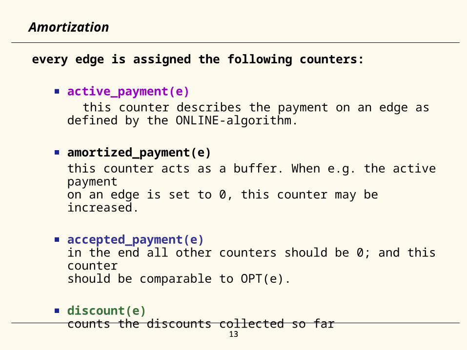
every edge is assigned the following counters:

active_payment(e) this counter describes the payment on an edge as

defined by the ONLINE-algorithm.

amortized_payment(e) this counter acts as a buffer. When e.g. the active payment

on an edge is set to 0, this counter may be increased.

accepted_payment(e)in the end all other counters should be 0; and this countershould be comparable to OPT(e).

discount(e)counts the discounts collected so far

Amortization

1414

Amortization

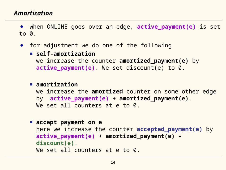
when ONLINE goes over an edge, active_payment(e) is set to 0.

for adjustment we do one of the following

self-amortizationwe increase the counter amortized_payment(e) by active_payment(e). We set discount(e) to 0.

amortization we increase the amortized-counter on some other edge by active_payment(e) + amortized_payment(e).We set all counters at e to 0.

accept payment on ehere we increase the counter accepted_payment(e) byactive_payment(e) + amortized_payment(e) - discount(e).We set all counters at e to 0.

1515

Amortization

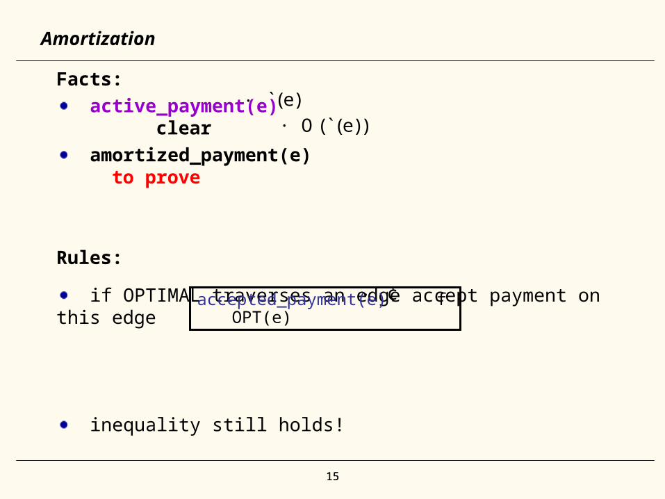
Facts:

active_payment(e) clear

amortized_payment(e) to prove

Rules:

if OPTIMAL traverses an edge accept payment on this edge

inequality still holds!

accepted_payment(e) f OPT(e)· ¢

· `(e)· O(`(e))

1616

Amortization

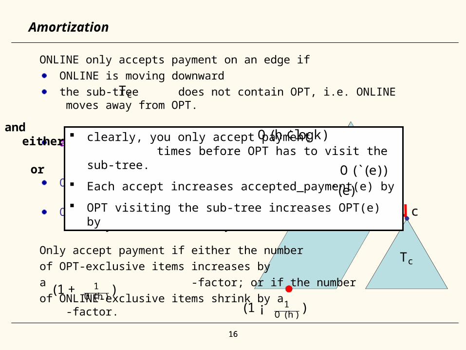
ONLINE only accepts payment on an edge if

ONLINE is moving downward

the sub-tree does not contain OPT, i.e. ONLINE moves away from OPT.

active(e)+amortized(e)-disount(e) <= 0

OPT-exclusive( ) items are those items in that are held by OPT but not by ONLINE.

ONLINE-exclusive( ) items are those held by ONLINE but not by OPT.

Only accept payment if either the number

of OPT-exclusive items increases by

a -factor; or if the number

of ONLINE-exclusive items shrink by a -factor.

Tc

c

Tc Tc

Tc

Tc

(1 + 1O (h)

)(1 ¡ 1

O (h))

and either

or

clearly, you only accept payment times before OPT has to visit the sub-tree.

Each accept increases accepted_payment(e) by

OPT visiting the sub-tree increases OPT(e) by

O(h ¢logk)

O(`(e))

`(e)

1717

Amortization

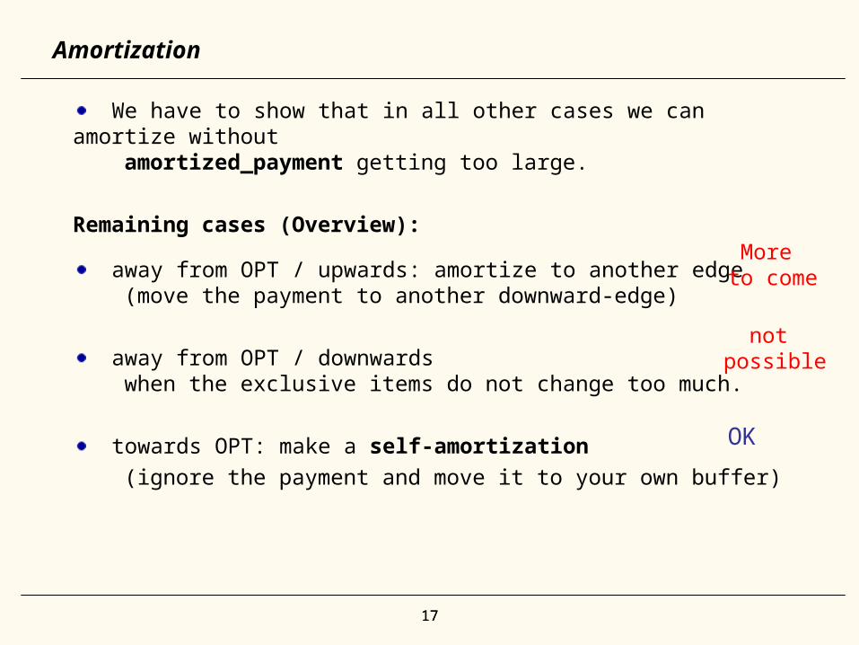
We have to show that in all other cases we can amortize without amortized_payment getting too large.

Remaining cases (Overview):

away from OPT / upwards: amortize to another edge (move the payment to another downward-edge)

away from OPT / downwards when the exclusive items do not change too much.

towards OPT: make a self-amortization

(ignore the payment and move it to your own buffer)OK

More to come

not possible

1818

Amortization

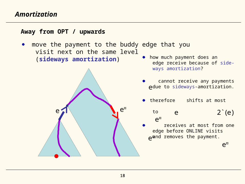
Away from OPT / upwards

move the payment to the buddy edge that you visit next on the same level (sideways amortization)

e e¤

how much payment does an edge receive because of side- ways amortization?

cannot receive any payments due to sideways-amortization.

therefore shifts at most to

receives at most from one edge before ONLINE visits and removes the payment.

e

e 2`(e)e¤

e¤

e¤

1919

Amortization

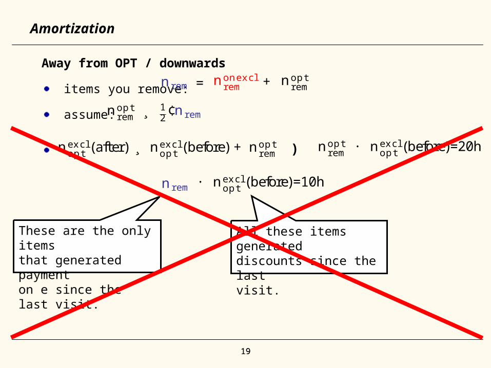
Away from OPT / downwards

items you remove:

assume:

=nrem nonexclrem + nopt

rem

noptrem nrem¸ 1

2¢

nexclopt (after) ¸ nexcl

opt (before) + noptrem

noptrem · nexcl

opt (before)=20h)

· nexclopt (before)=10hnrem

These are the only items that generated paymenton e since the last visit.

All these items generateddiscounts since the lastvisit.

2020

Amortization

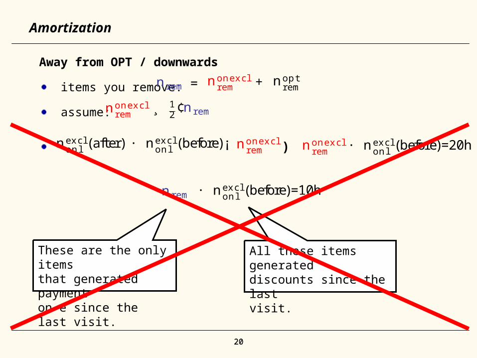
Away from OPT / downwards

items you remove:

assume:

=nrem nonexclrem + nopt

rem

nrem¸ 12¢nonexcl

rem

nonexclrem

nexclonl (after) · nexcl

onl (before)¡ ) · nexclonl (before)=20hnonexcl

rem

· nexclonl (before)=10hnrem

These are the only items that generated paymenton e since the last visit.

All these items generateddiscounts since the lastvisit.

2121

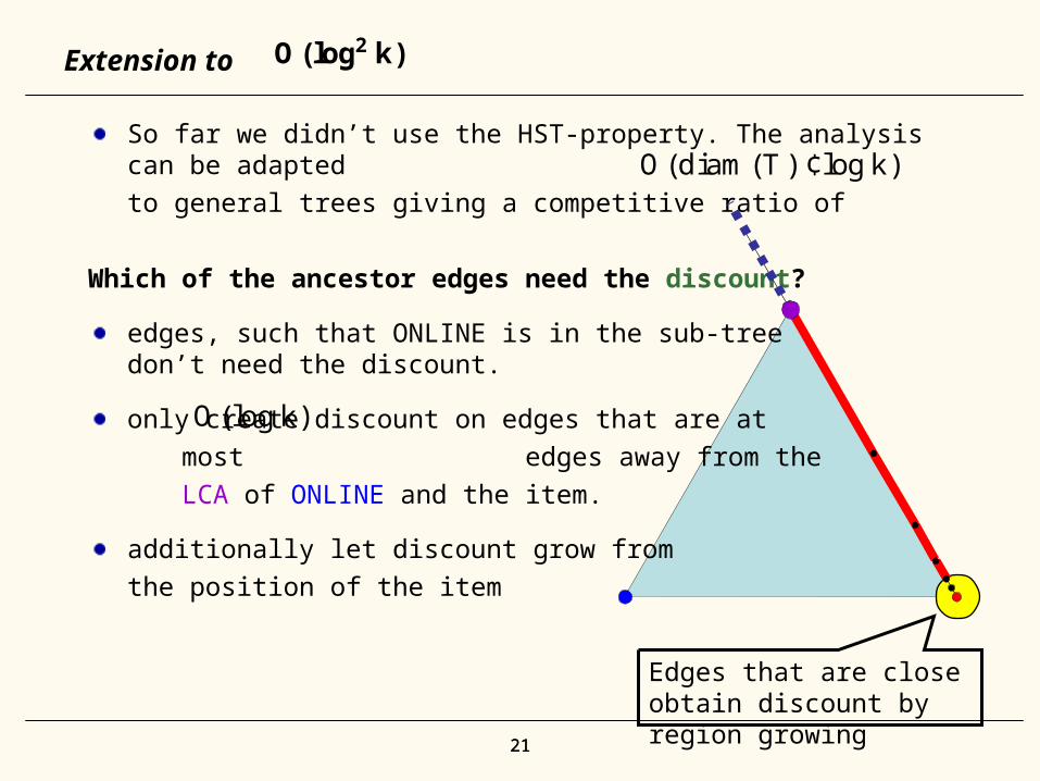
Extension to

So far we didn’t use the HST-property. The analysis can be adapted

to general trees giving a competitive ratio of

Which of the ancestor edges need the discount?

edges, such that ONLINE is in the sub-tree don’t need the discount.

only create discount on edges that are at

most edges away from the

LCA of ONLINE and the item.

additionally let discount grow from

the position of the item

O(log2 k)

O(diam(T ) ¢logk)

O(logk)

Edges that are close obtain discount by region growing

2222

Open Problems

Is it possible to reduce the competitive ratio toon the line / in arbitrary trees.

Can you remove the dependency on for arbitrarymetrics?

Is there a constant competitive ratio?

O(polylog(k))

k