11 Differential Equations and Proportionality - Cengagecollege.cengage.com/.../3e/students/ch11/401288_ch_11_722_764.pdf · CHAPTER Dynamics of Change: Differential Equations and

C H A P T E R

Dynamics of Change:DifferentialEquations andProportionality

722

Most of the functions that we have seenin this text have been motivated by

real-world phenomena. In many cases,it is the underlying rate of change thatdetermines whether the equation describinga phenomenon should be linear, quadratic,logistic, and so forth.

In this chapter we look at some applicationsof calculus that use information about ratesof change. We consider equations thatdescribe the forces that drive certain rates ofchange. Equations stating the behavior of arate of change (that is, equations involvingderivatives) are called differential equations.We look at differential equations graphicallyusing slope fields, numerically using Euler’smethod, and analytically using integration.

11

Concept Objectives

This chapter will help you understand theconcepts of

Constant and linear differential equationsDirect, inverse, and joint proportionalitySlope fieldsSeparable differential equationsEuler’s methodSecond-order differential equations

and you will learn to

Find and graph particular solutions todifferential equationsSet up differential equations using information about proportionalityUse slope fields to analyze a differential equation graphicallyUse Euler’s method to analyze a differentialequation numericallySolve first- and second-order differentialequations using antiderivatives

4362_HMC_Ch11_722-764 12/23/03 7:53 PM Page 722

Concept Application The rate of decay that a radioisotope undergoes dictates the amount of thatisotope left after a certain amount of time. It is this relationship that makes it possible for archeologists, geologists, and environmental engineers to useradioisotopes to help determine the age of artifacts and geological samples and to determine how much of a threat certain radioactive substances are to the environment. Activities 26 and 27 in Section 11.2 deal with developingdifferential equations from information about the decay of radioisotopes.

4362_HMC_Ch11_722-764 12/23/03 7:53 PM Page 723

724 CHAPTER 11 Dynamics of Change: Differential Equations and Proportionality

11.1 Differential Equations and Slope Fields

In Section 5.5 we saw how to use a known equation to develop a related-rates equationthat shows us the interconnection between different rates of change. Now we considerthe opposite process: using equations that describe rates of change to develop equa-tions that describe the situation. Equations that involve rates of change (derivatives)are called differential equations. The following equations are examples of differentialequations:

� �0.16p � 5.9x � 3.2y � 2.1s

� � 3xy � 4 � 2y

Differential Equations

Consider, for instance, the differential equation

� 63 mph

that describes the speed of a vehicle after x hours of traveling west on a straightstretch of interstate in North Dakota. Suppose we want an equation for the distancebetween the vehicle and the eastern border of the state after x hours. Because we are

given a derivative and wish to find a function y, we simply write the general anti-derivative:

y(x) � 63x � C miles

after x hours, where C represents the distance from the border when x � 0. Thisequation is the solution to the differential equation given above.

It is important to note that the solution of a differential equation is a functionwith derivatives that satisfy the differential equation. The solution is not a numeri-cal value. We define the function f to be a general solution to a differential equa-

tion � g(x, y) if the substitution of f(x) for y gives an identity (that is, a true

statement).

Differential Equation and General Solution

A differential equation involves one or more derivatives. A general solutionfor a differential equation is a function that has derivatives that satisfy thedifferential equation.

dydx

dydx

dydx

dydx

d 2ydx2

d 2ydx2

kln(t � 1.2)

dSdt

d 2sdt2

dydx

dcdp

Instructor NoteMake sure your studentsunderstand that a general solutionto a differential equation is anequation, not a number. Comparethis concept with that of a generalantiderivative.

4362_HMC_Ch11_722-764 12/23/03 7:53 PM Page 724

11.1 Differential Equations and Slope Fields 725

In the velocity example, we found y(x) � 63x � C miles to be a solution to

� 63 mph. To verify that this is indeed a general solution, we substitute y(x) into

the differential equation and obtain

(63x � C) � 63

63 � 63

The statement 63 � 63 is called an identity. This identity confirms that we have asolution. The C parameter in the solution is an arbitrary constant; it is used to desig-nate the family of functions that when differentiated, gives the differential equation.In practice, unique values for C will be determined by the initial conditions stated inthe specific problem that we are solving. In those cases, we call the solution a partic-ular solution.

The velocity example is a specific example of the simplest differential equation—

a constant differential equation that has the form � k, where k is a constant. To

solve this differential equation, we used our understanding of the relationshipbetween a rate-of-change function, the accumulation function of that rate of change,and the quantity function. That is, we found the solution to the differential equationby determining the general antiderivative of the rate-of-change function. Anothersimple differential equation, called a linear differential equation, has the form

� ax � b and is given in Example 1.

EXAMPLE 1 Finding Solutions for a Linear Differential Equation

Population Between 1900 and 2000 the population* of the United States wasgrowing at rate of 0.0181x � 1.129 million people per year where x is the number of years since 1900. In 1990 the population of the United States was 249.9 millionpeople.

a. Write a differential equation expressing the growth rate of the population withrespect to time.

b. Find a general solution for this differential equation.

c. Find a particular solution for this differential equation. Graph the differentialequation and the particular solution.

d. Use the particular solution to estimate the population in the year 2005.

Solution

a. Let P represent the population of the United States x years after 1900. The growthrate of the population is expressed by the differential equation

� 0.0181x � 1.129 million people per year

x years after 1900.

dPdx

dydx

dydx

ddx

dydx

*Based on data from Statistical Abstract, 1993, 1998, and 2001.

4362_HMC_Ch11_722-764 12/23/03 7:53 PM Page 725


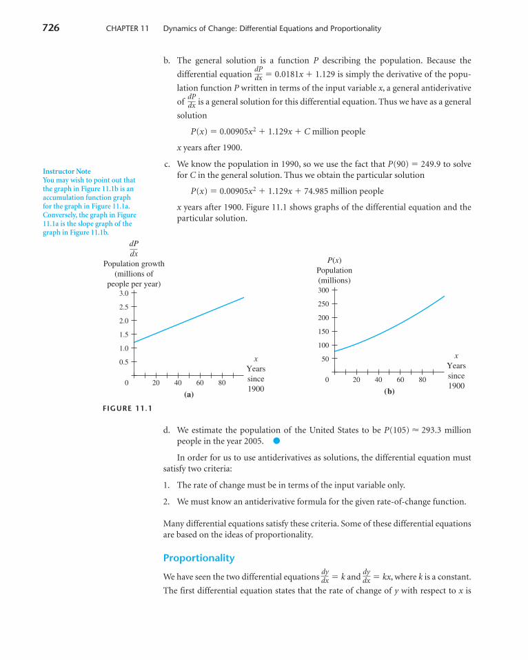
b. The general solution is a function P describing the population. Because the

differential equation � 0.0181x � 1.129 is simply the derivative of the popu-

lation function P written in terms of the input variable x, a general antiderivative

of is a general solution for this differential equation. Thus we have as a general

solution

P(x) � 0.00905x2 � 1.129x � C million people

x years after 1900.

c. We know the population in 1990, so we use the fact that P(90) � 249.9 to solvefor C in the general solution. Thus we obtain the particular solution

P(x) � 0.00905x2 � 1.129x � 74.985 million people

x years after 1900. Figure 11.1 shows graphs of the differential equation and theparticular solution.

FIGURE 11.1

d. We estimate the population of the United States to be P(105) � 293.3 millionpeople in the year 2005. ●

In order for us to use antiderivatives as solutions, the differential equation mustsatisfy two criteria:

1. The rate of change must be in terms of the input variable only.

2. We must know an antiderivative formula for the given rate-of-change function.

Many differential equations satisfy these criteria. Some of these differential equationsare based on the ideas of proportionality.

Proportionality

We have seen the two differential equations � k and � kx, where k is a constant.

The first differential equation states that the rate of change of y with respect to x is

dydx

dydx

xYearssince1900

(a)

0

0.5

Population growth(millions of

people per year)

dPdx

20 40 60 80

1.0

1.5

2.0

2.5

3.0

P(x)

xYearssince1900

(b)

0

50

Population(millions)

20 40 60 80

100

150

200

250

300

dPdx

dPdx

Instructor NoteYou may wish to point out that the graph in Figure 11.1b is anaccumulation function graph for the graph in Figure 11.1a.Conversely, the graph in Figure11.1a is the slope graph of thegraph in Figure 11.1b.

4362_HMC_Ch11_722-764 12/23/03 7:53 PM Page 726


constant. The second differential equation, � kx, states that the rate of change of ywith respect to x is proportional to the input x.

The idea of proportionality is one that is often used in setting up differential equa-tions. We say that a variable y is directly proportional to another variable x if there isa constant k such that y � kx. We call k the constant of proportionality. We use theterms proportional and directly proportional interchangeably.

For example, if A(t) � 23.50t dollars represents the amount it costs to purchase ttickets to a concert, then we say that the cost is directly proportional to the number oftickets purchased. In this case, 23.50 is the constant of proportionality.

Another type of proportionality occurs when a quantity y is related to a quantity x

by the equation y � , where k is a constant. In this case, we say that y is inverselyproportional to x.

The German physiologist Gustav Fechner* said that the rate of change of theintensity of a response R with respect to the intensity of a stimulus s is inversely pro-portional to the intensity of the stimulus. That is, there is some constant k such that

�

This differential equation, known as Fechner’s Law, says that if you are in a quietenvironment and a small bell rings, you will perceive the sound from the bell as beingrather loud, whereas if you are in a noisy environment and the same small bell rings,you will perceive the sound as being almost inaudible. Consider the followingresponse differential equation:

�

where the stimulus (input s) is measured in decibels and the response (output R)is measured on a scale of sound intensity where 0 represents no sound and 10

2.94s

dRds

ks

dRds

kx

Direct Proportionality

For input x and output y, y is directly proportional to x if there exists someconstant k such that y � kx. The constant k is called the constant ofproportionality.

dydx

Inverse Proportionality

For input x and output y, y is inversely proportional to x if there exists some

constant of proportionality k such that y � .kx

*D. N. Burghes and M. S. Borrie, Modelling with Differential Equations (Chichester, England: Ellis Hor-wood Limited, a division of Wiley, 1981).

4362_HMC_Ch11_722-764 12/23/03 7:53 PM Page 727


represents unbearably loud sound. A general solution of this differential equation issimply a general antiderivative:

R(s) � 2.94 ln s � C

where s is measured in decibels and is always positive.If the smallest sound that can be detected is 10 decibels, then we can use the ini-

tial condition R(10) � 0 to find a particular solution to the differential equation. Inthis case, the particular solution is

R(s) � 2.94 ln s � 6.77

where s is measured in decibels.

EXAMPLE 2 Evaluating the Constant of Proportionality

Sales Suppose that the total sales (in billions of dollars) of a computer product aregrowing in inverse proportion to ln(t � 1.2), where t is the number of years since theproduct was introduced. Sales totaled $53.2 billion by the end of the first year.

a. Write a differential equation representing the rate of change of sales with respectto time.

b. At the end of the first year, total sales were growing by 8.3 billion dollars per year.Find the constant of proportionality.

c. Can we write an explicit formula for the general solution of this differential equa-tion?

Solution

a. Let S(t) represent the total sales of the computer product t years after the productwas introduced. A differential equation representing the information given is

� billion dollars per year

where t is the number of years after the product was introduced.

b. We are told that � 8.3 billion dollars per year when t � 1. Using this fact, we

have

8.3 �

Thus the constant of proportionality is k � 6.544. The differential equation is



c. This differential equation expresses the derivative of S as a function of the inputvariable t. If we knew a formula for a general antiderivative of this function, thenwe could write a general solution of the differential equation. However, we do notknow such a formula. ●

6.544ln(t � 1.2)

dSdt

kln(1 � 1.2)

dSdt

kln(t � 1.2)

dSdt

4362_HMC_Ch11_722-764 12/23/03 7:53 PM Page 728


As in Example 2, even when the differential equation appears to be in a simpleform, we may not be able to find an explicit formula for its general solution. How-ever, we still can analyze such a differential equation graphically and numerically todevelop useful insight into the nature of the function and to estimate the solution.

Slope Fields

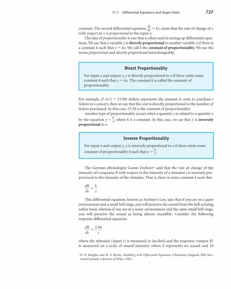
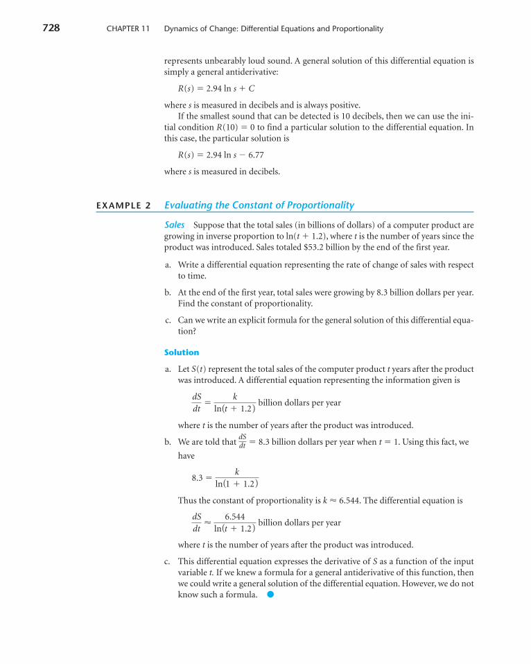
One way to obtain a graphical representation of a solution to a differential equationis to draw a slope field. A slope field is constructed by placing a grid on a portion ofthe Cartesian plane and, at each point on the grid, drawing a short line segmentwhose slope is determined by the differential equation. For instance, consider the dif-

ferential equation � 2x. At the point (1, 1), the slope of a solution to this equation

is 2x � 2(1) � 2, and at (�0.5, 2), the slope is 2x � 2(�0.5) � �1. Using the differen-tial equation to determine the slopes at points on a grid on a plane where �3 � x � 3and �6 � y � 6 and then sketching short line segments with those slopes at theappropriate points gives the slope field shown in Figure 11.2. (This construction is atedious process and is usually done with computer software.)

Particular solutions for the differential equation can be sketched by following theline segments in such a way that the solution curves are tangent to each of the

segments they meet. Figure 11.3 shows the graph of a particular solution for � 2x.

This particular solution goes through the point, or initial condition, (0, �1). We usethe term initial condition to refer to a known point on the graph of a particular solu-tion. Knowing an initial condition allows us to find a particular, rather than a gen-eral, solution.

FIGURE 11.2 FIGURE 11.3

The slope field indicates that at the point (0, �1), the derivative of the solution iszero. Thus the solution has a maximum, a minimum, or an inflection point at (0, �1).The slopes to the left of x � 0 indicate that the solution is decreasing toward (0, �1),and the slopes to the right of x � 0 indicate that the solution is increasing after itreaches (0, �1). Therefore (0, �1) is a minimum point. We form the solution graph byfollowing the general direction indicated by the slopes. You may find it helpful toconsider this as a more-sophisticated version of “connecting the dots.” Remember,however, that slopes in a slope field graph are plotted at only some, not all, points onthe plane.

x321−3 −2 −1

−6

−4

−2

2

4

6y

x321−3 −2 −1

−6

−4

−2

2

4

6y

dydx

dydx

Instructor NoteAlthough some technologies drawslope field graphs, we have chosennot to make the sketching of suchgraphs a part of our discussion.Instead, we always present a slopefield graph when needed.

Instructor NotePoint out to your students thesimilarities between knowing aninitial condition in order to sketcha particular solution and knowing a starting point in order to sketch a particular accumulation function.This is analogous to knowinginformation to find a specificantiderivative.

4362_HMC_Ch11_722-764 12/23/03 7:53 PM Page 729


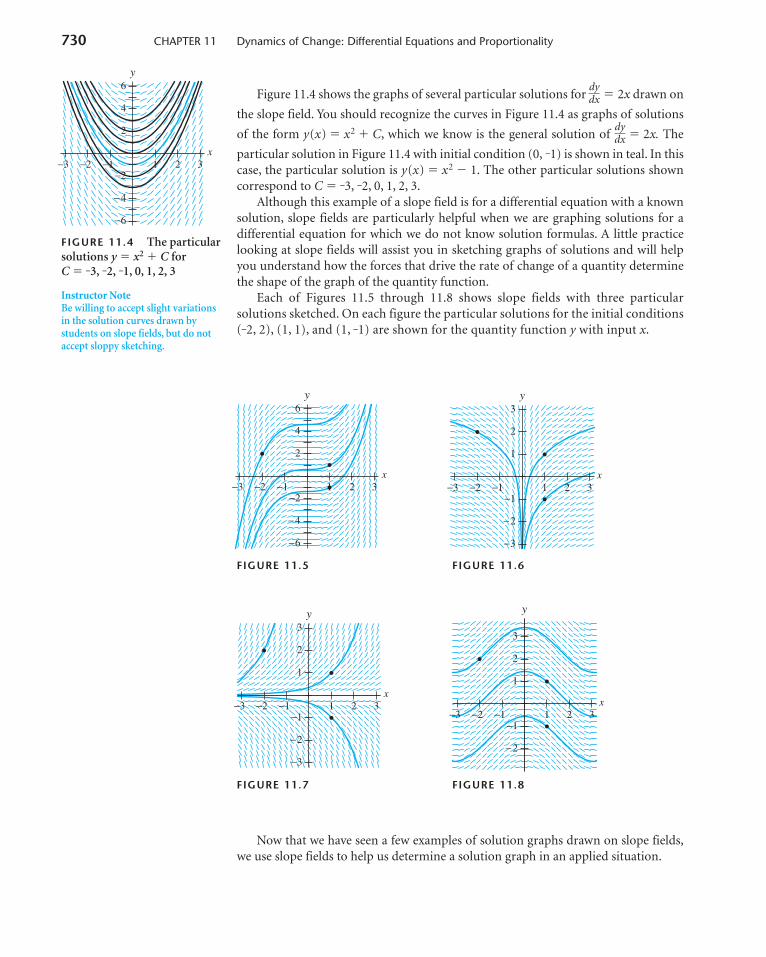
Figure 11.4 shows the graphs of several particular solutions for � 2x drawn on

the slope field. You should recognize the curves in Figure 11.4 as graphs of solutions

of the form y(x) � x2 � C, which we know is the general solution of � 2x. The

particular solution in Figure 11.4 with initial condition (0, �1) is shown in teal. In thiscase, the particular solution is y(x) � x2 � 1. The other particular solutions showncorrespond to C � �3, �2, 0, 1, 2, 3.

Although this example of a slope field is for a differential equation with a knownsolution, slope fields are particularly helpful when we are graphing solutions for adifferential equation for which we do not know solution formulas. A little practicelooking at slope fields will assist you in sketching graphs of solutions and will helpyou understand how the forces that drive the rate of change of a quantity determinethe shape of the graph of the quantity function.

Each of Figures 11.5 through 11.8 shows slope fields with three particular solutions sketched. On each figure the particular solutions for the initial conditions(�2, 2), (1, 1), and (1, �1) are shown for the quantity function y with input x.



Now that we have seen a few examples of solution graphs drawn on slope fields,we use slope fields to help us determine a solution graph in an applied situation.

x321−3 −2 −1

−2

−1

1

2

3

y

x321−3 −2 −1

−3

−2

−1

1

2

3y

x321−3 −2 −1

−3

−2

−1

1

2

3y

x321−3 −2 −1

−6

−4

−2

2

4

6y

dydx

dydx

Instructor NoteBe willing to accept slight variationsin the solution curves drawn bystudents on slope fields, but do notaccept sloppy sketching.

FIGURE 11.4 The particular solutions y � x2 � C for C � �3, �2, �1, 0, 1, 2, 3

x321−3 −2 −1

−6

−4

−2

2

4

6y

4362_HMC_Ch11_722-764 12/23/03 7:53 PM Page 730


EXAMPLE 3 Sketching Graphs of Particular Solutions on a Slope Field

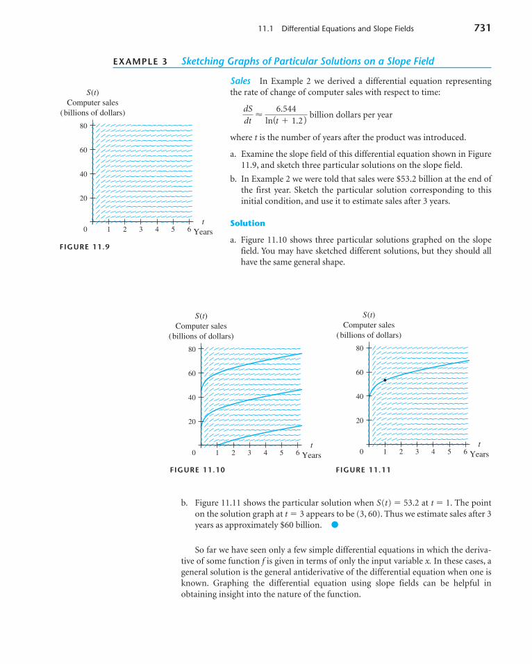
Sales In Example 2 we derived a differential equation representingthe rate of change of computer sales with respect to time:



a. Examine the slope field of this differential equation shown in Figure11.9, and sketch three particular solutions on the slope field.

b. In Example 2 we were told that sales were $53.2 billion at the end ofthe first year. Sketch the particular solution corresponding to thisinitial condition, and use it to estimate sales after 3 years.

Solution

a. Figure 11.10 shows three particular solutions graphed on the slopefield. You may have sketched different solutions, but they should allhave the same general shape.


b. Figure 11.11 shows the particular solution when S(t) � 53.2 at t � 1. The pointon the solution graph at t � 3 appears to be (3, 60). Thus we estimate sales after 3years as approximately $60 billion. ●

So far we have seen only a few simple differential equations in which the deriva-tive of some function f is given in terms of only the input variable x. In these cases, ageneral solution is the general antiderivative of the differential equation when one isknown. Graphing the differential equation using slope fields can be helpful inobtaining insight into the nature of the function.

1 2 3 4 5 60

20

40

60

80

tYears

Computer sales(billions of dollars)

S(t)

1 2 3 4 5 6t

Years


S(t)

0

20

40

60

80

6.544ln(t � 1.2)

dSdt

FIGURE 11.9

tYears0

20


1 2 3 4 5 6

40

60

80

S(t)

4362_HMC_Ch11_722-764 12/23/03 7:53 PM Page 731


11.1 Concept Inventory

Solutions to differential equations of the form

� k


� f(x)

Direct proportionality

Inverse proportionality

Slope fields

11.1 Activities

For Activities 1 through 4, write an equation or differen-tial equation for the given information.

1. The cost c to fill your gas tank is directly propor-tional to the number of gallons g your tank willhold.

2. The marginal cost of producing window panes(that is, the rate of change of cost c with respect tothe number of units produced) is inversely propor-tional to the number of panes p produced.

3. Barometric pressure p is changing with respect toaltitude a at a rate that is proportional to the altitude.

4. The rate of change of the cost c of mailing a first-class letter with respect to the weight of the letter isconstant.

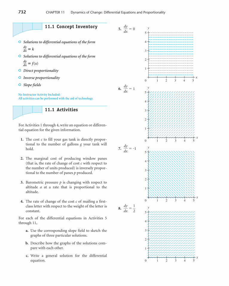
For each of the differential equations in Activities 5through 11,

a. Use the corresponding slope field to sketch thegraphs of three particular solutions.

b. Describe how the graphs of the solutions com-pare with each other.

c. Write a general solution for the differentialequation.

dydx

dydx

5. � 0

6. � 1

7. � �1

8. �

1

1

2

3

4

5

0 2 3 4 5x

y12

dydx

1

1

2

3

4

5

0 2 3 4 5x

ydydx

1

1

2

3

4

5

0 2 3 4 5x

ydydx

1

1

2

3

4

5

0 2 3 4 5x

ydydx

No Instructor Activity Included:All activities can be performed with the aid of technology.

4362_HMC_Ch11_722-764 12/23/03 7:53 PM Page 732


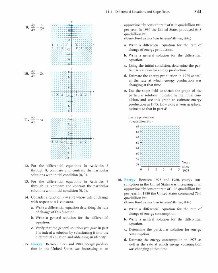
9. � x

10. � 2x

11. � �x

12. For the differential equations in Activities 5through 8, compare and contrast the particularsolutions with initial condition (0, 0).

13. For the differential equations in Activities 9through 11, compare and contrast the particularsolutions with initial condition (0, 0).

14. Consider a function y � f(x) whose rate of changewith respect to x is constant.

a. Write a differential equation describing the rateof change of this function.

b. Write a general solution for the differentialequation.

c. Verify that the general solution you gave in partb is indeed a solution by substituting it into thedifferential equation and obtaining an identity.

15. Energy Between 1975 and 1980, energy produc-tion in the United States was increasing at an

x−4 −3 −2 −1

−8

−6

−4

−2 4321

y8

6

4

2

dydx

x−4 −3 −2 −1

−8

−6

−4

−2 4321

y8

6

4

2

dydx

x−4 −3 −2 −1

−8

−6

−4

−2 4321

y8

6

4

2

12

dydx

approximately constant rate of 0.98 quadrillion Btuper year. In 1980 the United States produced 64.8quadrillion Btu.(Source: Based on data from Statistical Abstract, 1994.)

a. Write a differential equation for the rate ofchange of energy production.


c. Using the initial condition, determine the par-ticular solution for energy production.

d. Estimate the energy production in 1975 as wellas the rate at which energy production waschanging at that time.

e. Use the slope field to sketch the graph of theparticular solution indicated by the initial con-dition, and use this graph to estimate energyproduction in 1975. How close is your graphicalestimate to that in part d?

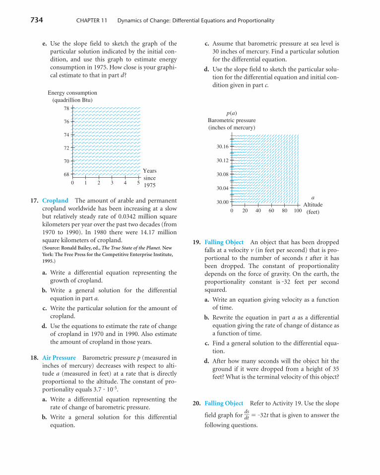
16. Energy Between 1975 and 1980, energy con-sumption in the United States was increasing at anapproximately constant rate of 1.08 quadrillion Btuper year. In 1980 the United States consumed 76.0quadrillion Btu.(Source: Based on data from Statistical Abstract, 1994.)

a. Write a differential equation for the rate ofchange of energy consumption.


c. Determine the particular solution for energyconsumption.

d. Estimate the energy consumption in 1975 aswell as the rate at which energy consumptionwas changing at that time.

Energy production(quadrillion Btu)

Yearssince197510 32 54

65

64

63

62

61

60

59

58

4362_HMC_Ch11_722-764 12/23/03 7:53 PM Page 733


e. Use the slope field to sketch the graph of theparticular solution indicated by the initial con-dition, and use this graph to estimate energyconsumption in 1975. How close is your graphi-cal estimate to that in part d?

17. Cropland The amount of arable and permanentcropland worldwide has been increasing at a slowbut relatively steady rate of 0.0342 million squarekilometers per year over the past two decades (from1970 to 1990). In 1980 there were 14.17 millionsquare kilometers of cropland.(Source: Ronald Bailey, ed., The True State of the Planet. NewYork: The Free Press for the Competitive Enterprise Institute,1995.)

a. Write a differential equation representing thegrowth of cropland.

b. Write a general solution for the differentialequation in part a.

c. Write the particular solution for the amount ofcropland.

d. Use the equations to estimate the rate of changeof cropland in 1970 and in 1990. Also estimatethe amount of cropland in those years.

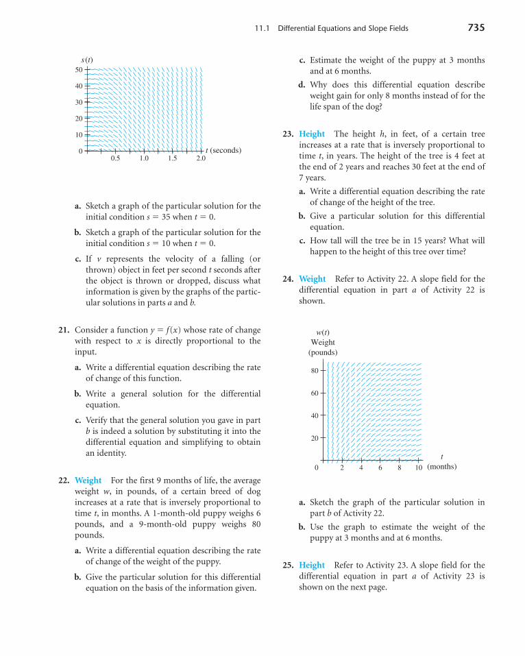
18. Air Pressure Barometric pressure p (measured ininches of mercury) decreases with respect to alti-tude a (measured in feet) at a rate that is directlyproportional to the altitude. The constant of pro-portionality equals 3.7 � 10�5.

a. Write a differential equation representing therate of change of barometric pressure.

b. Write a general solution for this differentialequation.

Energy consumption(quadrillion Btu)

Yearssince197510 32 54

78

76

74

72

70

68

c. Assume that barometric pressure at sea level is30 inches of mercury. Find a particular solutionfor the differential equation.

d. Use the slope field to sketch the particular solu-tion for the differential equation and initial con-dition given in part c.

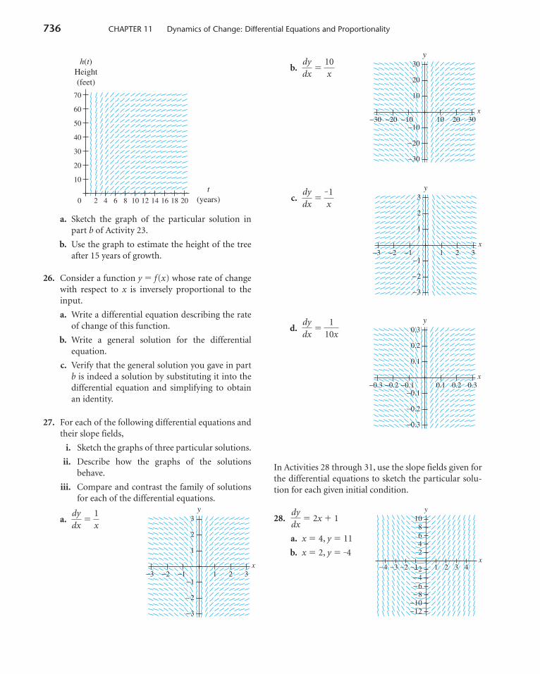
19. Falling Object An object that has been droppedfalls at a velocity v (in feet per second) that is pro-portional to the number of seconds t after it hasbeen dropped. The constant of proportionalitydepends on the force of gravity. On the earth, theproportionality constant is �32 feet per secondsquared.

a. Write an equation giving velocity as a functionof time.

b. Rewrite the equation in part a as a differentialequation giving the rate of change of distance asa function of time.

c. Find a general solution to the differential equa-tion.

d. After how many seconds will the object hit theground if it were dropped from a height of 35feet? What is the terminal velocity of this object?

20. Falling Object Refer to Activity 19. Use the slope

field graph for � �32t that is given to answer the

following questions.

dsdt

p(a)Barometric pressure(inches of mercury)

aAltitude

(feet)200 6040 10080

30.16

30.12

30.08

30.04

30.00

4362_HMC_Ch11_722-764 12/23/03 7:53 PM Page 734


a. Sketch a graph of the particular solution for theinitial condition s � 35 when t � 0.

b. Sketch a graph of the particular solution for theinitial condition s � 10 when t � 0.

c. If v represents the velocity of a falling (orthrown) object in feet per second t seconds afterthe object is thrown or dropped, discuss whatinformation is given by the graphs of the partic-ular solutions in parts a and b.

21. Consider a function y � f(x) whose rate of changewith respect to x is directly proportional to theinput.



c. Verify that the general solution you gave in partb is indeed a solution by substituting it into thedifferential equation and simplifying to obtainan identity.

22. Weight For the first 9 months of life, the averageweight w, in pounds, of a certain breed of dogincreases at a rate that is inversely proportional totime t, in months. A 1-month-old puppy weighs 6pounds, and a 9-month-old puppy weighs 80pounds.

a. Write a differential equation describing the rateof change of the weight of the puppy.

b. Give the particular solution for this differentialequation on the basis of the information given.

s (t)

30

40

50

0

10

20

t (seconds)0.5 1.0 1.5 2.0

c. Estimate the weight of the puppy at 3 monthsand at 6 months.

d. Why does this differential equation describeweight gain for only 8 months instead of for thelife span of the dog?

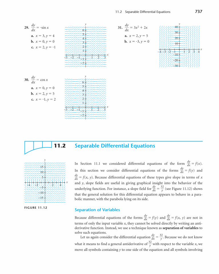
23. Height The height h, in feet, of a certain treeincreases at a rate that is inversely proportional totime t, in years. The height of the tree is 4 feet atthe end of 2 years and reaches 30 feet at the end of7 years.

a. Write a differential equation describing the rateof change of the height of the tree.

b. Give a particular solution for this differentialequation.

c. How tall will the tree be in 15 years? What willhappen to the height of this tree over time?

24. Weight Refer to Activity 22. A slope field for thedifferential equation in part a of Activity 22 isshown.

a. Sketch the graph of the particular solution inpart b of Activity 22.

b. Use the graph to estimate the weight of thepuppy at 3 months and at 6 months.

25. Height Refer to Activity 23. A slope field for thedifferential equation in part a of Activity 23 isshown on the next page.

w(t)

t(months)

Weight(pounds)

2 64 108

80

60

40

20

0

4362_HMC_Ch11_722-764 12/23/03 7:53 PM Page 735


a. Sketch the graph of the particular solution inpart b of Activity 23.

b. Use the graph to estimate the height of the treeafter 15 years of growth.

26. Consider a function y � f(x) whose rate of changewith respect to x is inversely proportional to theinput.




27. For each of the following differential equations andtheir slope fields,

i. Sketch the graphs of three particular solutions.

ii. Describe how the graphs of the solutionsbehave.

iii. Compare and contrast the family of solutionsfor each of the differential equations.

a. �

x321−3 −2 −1

−3

−2

−1

1

2

3y1

xdydx

t(years)

h(t)Height(feet)

4 128 20162 106 1814

70

60

50

40

30

20

10

0

b. �

c. �

d. �

In Activities 28 through 31, use the slope fields given forthe differential equations to sketch the particular solu-tion for each given initial condition.

28. � 2x � 1

a. x � 4, y � 11

b. x � 2, y � �4x

y

−4 −3 −2 −1 1 2 3 4

−12−10−8−6− 4−2

2468

10dydx

x0.30.20.1−0.3 −0.2 −0.1

−0.3

−0.2

−0.1

0.1

0.2

0.3y1

10xdydx

x321−3 −2 −1

−3

−2

−1

1

2

3y�1

xdydx

x302010−30 −20 −10

−30

−20

−10

10

20

30y

10x

dydx

4362_HMC_Ch11_722-764 12/23/03 7:53 PM Page 736

11.2 Separable Differential Equations 737

29. � �sin x

a. x � 3, y � 4

b. x � 0, y � 0

c. x � 2, y � �1

30. � cos x

a. x � 0, y � 0

b. x � 2, y � 5

c. x � �1, y � 2

x

y

321−3 −2 −1

−2−1

123456

dydx

x

y

321−3 −2 −1

−2−1

123456

dydx

31. � 3x2 � 2x

a. x � 2, y � 5

b. x � �3, y � 0

x

y

−4 −3 −2 −1 1 2 3 4

−30

−20

−10

10

20

30

40dydx

11.2 Separable Differential Equations

In Section 11.1 we considered differential equations of the form � f(x).

In this section we consider differential equations of the forms � f(y) and

� f(x, y). Because differential equations of these types give slope in terms of x

and y, slope fields are useful in giving graphical insight into the behavior of the

underlying function. For instance, a slope field for � (see Figure 11.12) shows

that the general solution for this differential equation appears to behave in a para-bolic manner, with the parabola lying on its side.

Separation of Variables

Because differential equations of the forms � f(y) and � f(x, y) are not in

terms of only the input variable x, they cannot be solved directly by writing an anti-derivative function. Instead, we use a technique known as separation of variables tosolve such equations.

Let us again consider the differential equation � . Because we do not know

what it means to find a general antiderivative of with respect to the variable x, we

move all symbols containing y to one side of the equation and all symbols involving

32y

32y

dydx

dydx

dydx

32y

dydx

dydx

dydx

dydx

FIGURE 11.12

x

y

42−4 −2

−15

−10

−5

5

10

15

4362_HMC_Ch11_722-764 12/23/03 7:53 PM Page 737


x to the other side of the equation. This procedure is known as separating the vari-ables. In this case, we have

y dy � 32dx

Now that the equation has the variables separated, we take antiderivatives of bothsides of the equation.

y dy � 32dx

y2 � c1 � 32x � c2

where c1 and c2 are both constants. Combining the constants and solving for y2 yields

y2 � 64x � C

Finally, we write the solution equation giving y in terms of x by taking the square rootof both sides of the equation.

y � �

This equation does indeed yield the two sides of a horizontal parabola, as theslope field indicates. In this case, y is not a function of x because a single value of xcould yield two different values of y.

Differential Equations Modeling Constant Percentage Change

Any time that percentage growth is constant, the situation can be described by the

differential equation � ky, where k is the constant percentage rate of change.

Because constant percentage growth characterizes exponential functions, the solu-tion to this differential equation is y � aekx. Example 1 illustrates the solution to dif-ferential equations of this form.

EXAMPLE 1 Solving Differential Equations Using Separation of Variables

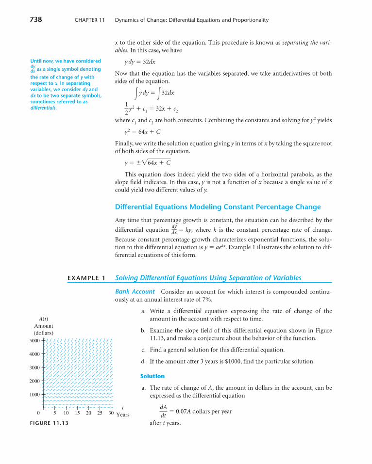
Bank Account Consider an account for which interest is compounded continu-ously at an annual interest rate of 7%.

a. Write a differential equation expressing the rate of change of theamount in the account with respect to time.

b. Examine the slope field of this differential equation shown in Figure11.13, and make a conjecture about the behavior of the function.

c. Find a general solution for this differential equation.

d. If the amount after 3 years is $1000, find the particular solution.

Solution

a. The rate of change of A, the amount in dollars in the account, can beexpressed as the differential equation

� 0.07A dollars per year

after t years.

dAdt

dydx

�64x � C

12

��

Until now, we have considered

as a single symbol denoting

the rate of change of y withrespect to x. In separatingvariables, we consider dy and dx to be two separate symbols,sometimes referred to asdifferentials.

dydx

FIGURE 11.13

5 10 15 20 25 300

5000

4000

3000

2000

1000

Amount(dollars)

A(t)

tYears

4362_HMC_Ch11_722-764 12/23/03 7:53 PM Page 738


b. This slope field indicates a horizontal asymptote at A � 0 and growth thatincreases as t increases. This behavior is indicative of an exponential model.

c. To solve this equation, we use the technique of separating variables:

dA � 0.07dt

Determining general antiderivatives of both sides, we have

dA � 0.07dt

which gives

ln A � c1 � 0.07t � c2

Combining the constants yields

ln A � 0.07t � C

Recalling from algebra that ln x � y is equivalent to x � e y, we have

A � e(0.07t�C)

� e0.07t eC

Replacing the constant eC with the constant a gives the general solution

A � ae0.07t dollars

after t years.

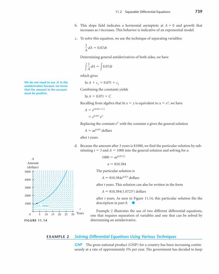
d. Because the amount after 3 years is $1000, we find the particular solution by sub-stituting t � 3 and A � 1000 into the general solution and solving for a.

1000 � ae0.07(3)

a � 810.584

The particular solution is

A � 810.584e0.07t dollars

after t years. This solution can also be written in the form

A � 810.584(1.0725t) dollars

after t years. As seen in Figure 11.14, this particular solution fits thedescription in part b. ●

Example 2 illustrates the use of two different differential equations,one that requires separation of variables and one that can be solved bydetermining an antiderivative.

EXAMPLE 2 Solving Differential Equations Using Various Techniques

GNP The gross national product (GNP) for a country has been increasing contin-uously at a rate of approximately 5% per year. The government has decided to keep

�1A�

1A

We do not need to use �A� in theantiderivative because we knowthat the amount in the accountmust be positive.

FIGURE 11.14

5 10 15 20 25 300

5000

4000

3000

2000

1000

AAmount(dollars)

(3, 1000)t

Years

4362_HMC_Ch11_722-764 12/23/03 7:53 PM Page 739


the growth in the rate of deficit spending proportional to the GNP. Last year the GNPwas $3 billion, and the country’s national debt was $2.3 billion. The government hasmandated that this year’s national debt be held at $2.4 billion dollars.

a. Express the country’s GNP growth as a differential equation, and find the solution.

b. Express the rate of change of the country’s national debt as a differential equa-tion, and find the solution.

c. Evaluate the solutions for t � 2, and interpret the answers.

Solution

a. Let G represent the GNP in billions of dollars. Then � 0.05G billion dollars

per year represents the rate of change of the GNP after t years. The solution isfound by separating variables.

dG � 0.05 dt

yields

ln G � 0.05t � C

which can be rewritten as

G � ae0.05t billion dollars

If we consider t to be the number of years since last year, then a � 3 since theGNP in year 0 (last year) was $3 billion. Thus the solution to the differentialequation is

G � 3e0.05t billion dollars

after t years.

b. Let D be the national debt in billions of dollars. The statement “the growth rate ofdeficit spending is proportional to the GNP” can be translated into mathematicalsymbols as

� kG billion dollars per year

after t years, where k is the constant of proportionality. Note that at this point wedo not have the information needed to solve for k. However, we have the infor-mation to solve for k once we find a general solution. Knowing a function for G,we substitute this into the differential equation:

� k(3e0.05t)

Because this differential equation gives the derivative of D in terms of only theinput t, we do not need to use separation of variables but can proceed by writinga general antiderivative:

D(t) � � C � 60ke0.05t � C billion dollars3ke0.05t

0.05

dDdt

dDdt

1G

dGdt

Instructor NoteThe details of how to rewrite ln G � 0.05t � C as G � ae0.05t

are given in part c of Example 1.

4362_HMC_Ch11_722-764 12/23/03 7:53 PM Page 740


after t years. We now have two constants, k and C, to determine, so we must cre-ate a system of two equations that we can solve simultaneously. Because thenational debt last year (when t � 0) was $2.3 billion, we substitute this informa-tion into D:

2.3 � 60ke0 � C � 60k � C (1)

Also, the national debt is $2.4 billion when t � 1, so

2.4 � 60ke0.05 � C (2)

Solving equation 1 for C and substituting into equation 2 give the equation

2.4 � 60ke0.05 � (2.3 � 60k)

or

0.1 � (60e0.05 � 60)k

k �

Thus k � 0.0325. Using this value of k in equation 1 gives

C � 2.3 � 60(0.0325) � 0.3496

Thus we have the particular solution

D(t) � 1.9504e0.05t � 0.3496 billion dollars

after t years.

c. When t � 2, G(2) � $3.3 billion and D(2) � $2.5 billion. In 2 years, the GNPwill be approximately $3.3 billion, and the national debt should be held toapproximately $2.5 billion. ●

Joint Proportionality

Section 11.1 introduced two forms of proportionality: direct and inverse. Now weconsider a third form of proportionality. When a quantity y is proportional to theproduct of two other quantities x and z, that is, when there is some constant k suchthat y � kxz, we say the quantity y is jointly proportional to the quantities x and z.

Example 3 illustrates the concept of joint proportionality as it is used in psychology.

Joint Proportionality

For inputs x and z and output y, y is jointly proportional to x and z if thereexists some constant of proportionality k such that y � kxz.

0.160e0.05 � 60

Strengtheningthe Concepts:

SolvingSimultaneous

Equations

WEB/CD

4362_HMC_Ch11_722-764 12/23/03 7:53 PM Page 741


EXAMPLE 3 Solving an Equation Involving Joint Proportionality

Stimulus Response The Fechner Law relates response to stimulus. A differentmodel that is used to describe this relationship is the Brentano-Stevens Law. This lawsays that the level of response R changes according to a joint proportionality between

the level of the response and the inverse of s, the level of the stimulus. That is, � k

for some constant k.Consider the following differential equation that describes a person’s perception

of the intensity of sound:

�

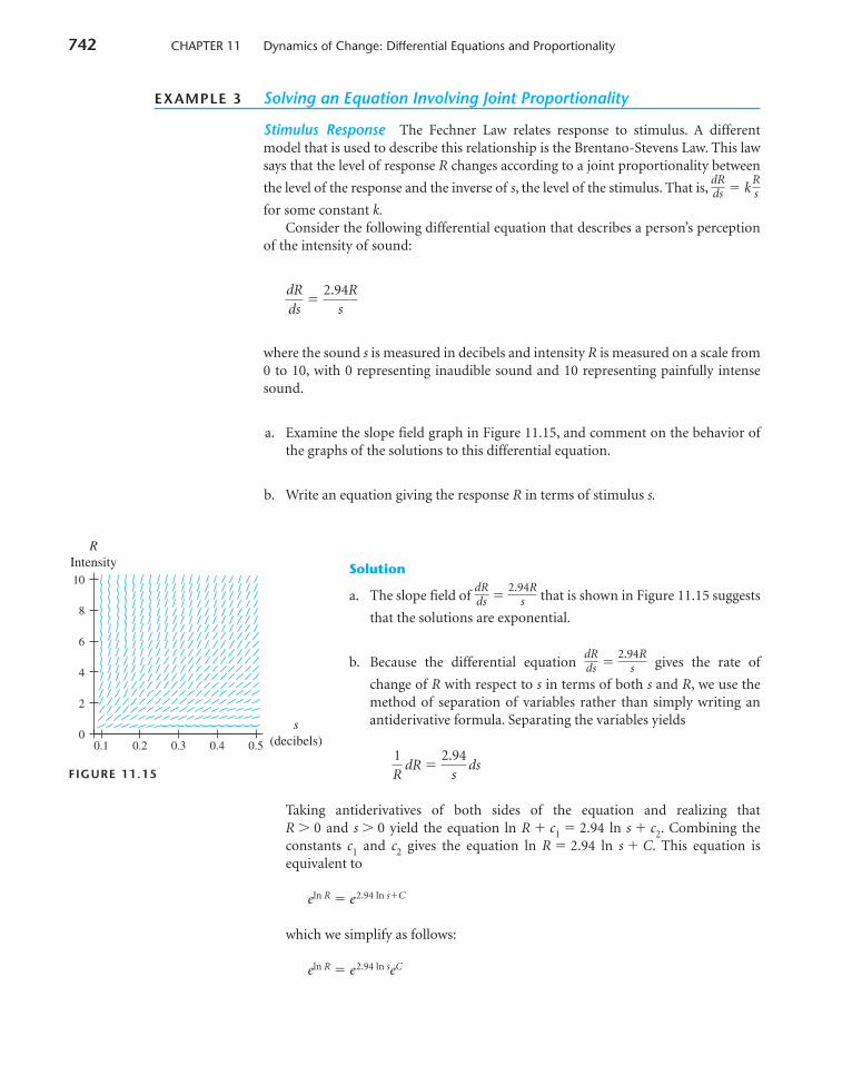
where the sound s is measured in decibels and intensity R is measured on a scale from0 to 10, with 0 representing inaudible sound and 10 representing painfully intensesound.

a. Examine the slope field graph in Figure 11.15, and comment on the behavior ofthe graphs of the solutions to this differential equation.

b. Write an equation giving the response R in terms of stimulus s.

Solution

a. The slope field of � that is shown in Figure 11.15 suggests

that the solutions are exponential.

b. Because the differential equation � gives the rate of

change of R with respect to s in terms of both s and R, we use themethod of separation of variables rather than simply writing anantiderivative formula. Separating the variables yields

dR � ds

Taking antiderivatives of both sides of the equation and realizing that R � 0 and s � 0 yield the equation ln R � c1 � 2.94 ln s � c2. Combining the constants c1 and c2 gives the equation ln R � 2.94 ln s � C. This equation isequivalent to

eln R � e2.94 ln s�C

which we simplify as follows:

eln R � e2.94 ln seC

2.94s

1R

2.94Rs

dRds

2.94Rs

dRds

2.94Rs

dRds

Rs

dRds

FIGURE 11.15

s(decibels)0.1 0.2 0.3 0.4 0.5

10

8

6

4

2

0

RIntensity

4362_HMC_Ch11_722-764 12/23/03 7:53 PM Page 742


eln R � (eln s)2.94eC

R � s2.94eC

Replacing eC with the constant a gives the general solution as

R � as2.94

where s is measured in decibels and a is a constant. ●

Logistic Models and Their Differential Equations

We have seen differential equations that lead to linear, quadratic, logarithmic, andexponential models. What does a differential equation that yields a logistic modellook like? To help us better understand the underlying differential equation, recall therole of the limiting value L in a logistic model

y(x) �

As we saw in Chapter 2, the logistic model may be used to study the spread of a virusin a network of computers. The virus initially spreads exponentially because the firstcomputer infects another, then these two computers infect two others, then the fourof them infect four others, and so on. At some point, the computers that have thevirus contact only others that are also infected instead of uninfected computers, andthe exponential sequence is broken. Eventually, the number of infected computers isclose to the limiting value L.

The rate of change of the number of infected computers depends on two things:the number y of computers already infected and the number L � y of computers notyet infected. Thus the rate of change is jointly proportional to the number of com-puters already infected and the number of uninfected computers remaining. We candescribe the spread of a virus with the differential equation

� ky(L � y)

where L is the number of computers in the group and k is the constant of propor-tionality. It is also common to refer to the limiting value L as the carrying capacity ofthe system or as the saturation level.

A slope graph of a differential equation of the form � ky(L � y) gives us

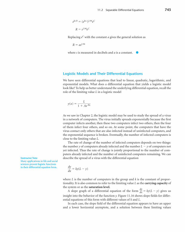
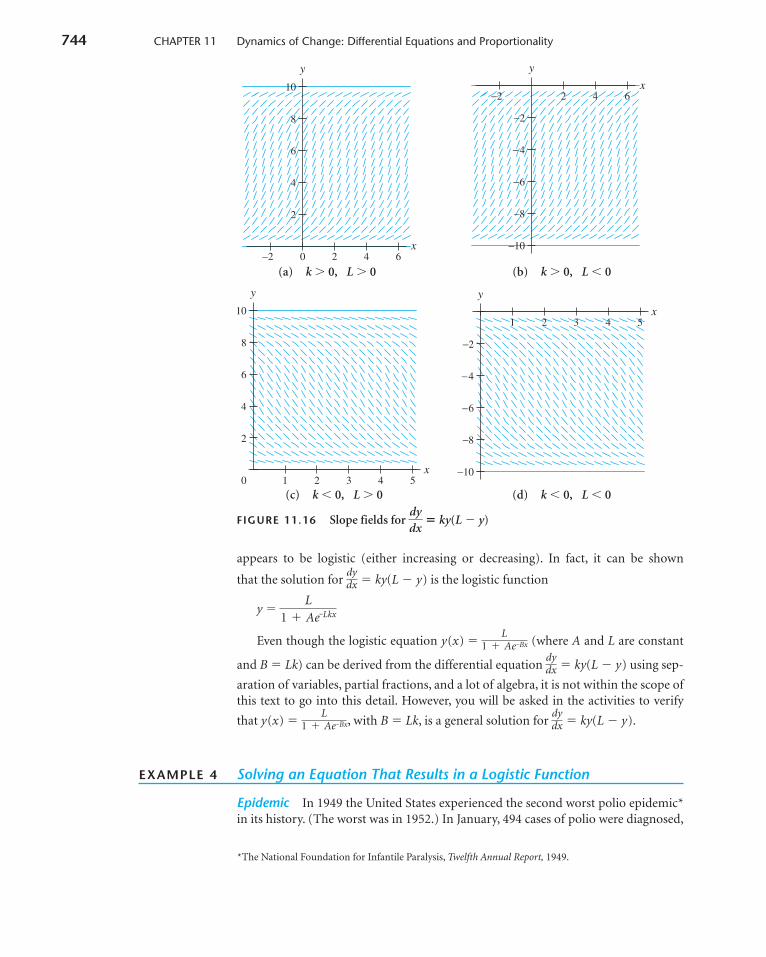
insight into the behavior of the function y. Figure 11.16 shows slope fields for differ-ential equations of this form with different values of k and L.

In each case, the slope field of the differential equation appears to have an upperand a lower horizontal asymptote, and a solution between these limiting values

dydx

dydx

L1 � Ae�Bx

Instructor NoteMany applications in life and socialsciences present logistic functionsin their differential equation form.

4362_HMC_Ch11_722-764 12/23/03 7:53 PM Page 743


FIGURE 11.16 Slope fields for � ky(L � y)

appears to be logistic (either increasing or decreasing). In fact, it can be shown

that the solution for � ky(L � y) is the logistic function

y �

Even though the logistic equation y(x) � (where A and L are constant

and B � Lk) can be derived from the differential equation � ky(L � y) using sep-

aration of variables, partial fractions, and a lot of algebra, it is not within the scope ofthis text to go into this detail. However, you will be asked in the activities to verify

that y(x) � , with B � Lk, is a general solution for � ky(L � y).

EXAMPLE 4 Solving an Equation That Results in a Logistic Function

Epidemic In 1949 the United States experienced the second worst polio epidemic*in its history. (The worst was in 1952.) In January, 494 cases of polio were diagnosed,

dydx

L1 � Ae�Bx

dydx

L1 � Ae�Bx

L1 � Ae�Lkx

dydx

dydx

2

4

6

8

10

0 2−2 4 6x

y

2−2

−2

−4

−6

−8

−10

4 6x

y

2

4

6

8

10

0 1 2 3 4 5x

y

−8

−6

−4

−2

−10

1 2 3 4 5x

y

(a) k � 0, L � 0 (b) k � 0, L 0

(c) k 0, L � 0 (d) k 0, L 0

*The National Foundation for Infantile Paralysis, Twelfth Annual Report, 1949.

4362_HMC_Ch11_722-764 12/23/03 7:53 PM Page 744


and by December, a total of 42,375 cases had been diagnosed. Assume that the spreadof polio followed the general principle that the rate of spread was jointly propor-tional to the number of infected people and the number of uninfected people. Alsoassume that the carrying capacity for polio in the United States in 1949 was approxi-mately 43,000 people.

a. Write a differential equation describing the spread of polio.

b. Determine a particular solution for this differential equation.

Solution

a. Let P(m) be the number of polio cases diagnosed by the end of the mth month of1949, and let k be the constant of proportionality. A differential equation describ-ing the spread of polio is

� kP(43,000 � P) cases per month

Because we are given information about the number of cases, not informationconcerning the rate of change of the number of cases, we cannot find the con-stant of proportionality at this point.

b. A general solution for this differential equation is the logistic equation

P(m) � cases

diagnosed by the end of the mth month of 1949. This equation contains two con-stants, A and k, for which we must solve. We are given the two points (1, 494) and(12, 42,375). Substituting these into the logistic equation, we obtain a system oftwo equations that we can solve simultaneously for the two constants, A and k.The two equations are

494 � (3)

42,375 � (4)

Solving equation 3 for A and substituting into equation 4 yield

42,375 �

Solving this equation for k yields k � 1.83328271 � 10�5, or B � Lk � 0.788312.Substituting k into equation 3 and solving for A yield A � 189.2704. Thus wehave the particular solution

P(m) � cases

diagnosed by the mth month of 1949. ●

43,0001 � 189.2704e�0.788312m

43,000

1 � �42,506e43,000k

494 �e�516,000k

43,0001 � Ae�516,000k

43,0001 � Ae�43,000k

43,0001 � Ae�43,000km

dPdm

4362_HMC_Ch11_722-764 12/23/03 7:53 PM Page 745

Separation of variables often yields a solution when we are considering differen-

tial equations of the form � f(y) or � f(x, y). Slope fields usually give

graphical insight into the behavior of the underlying function, and in the case where

� ky(L � y), we have a specific equation that gives the solution. However, there

are many differential equations for which graphical and algebraic methods of deter-mining particular solutions are beyond the scope of this book. In fact, there are manydifferential equations for which algebraic solution methods fail. In such cases, we relyon numerical techniques, one of which is discussed in the next section.

dydx

dydx

dydx




� f(x, y)


� ky


� ky(L � y)

Separation of variables

Joint proportionality

11.2 Activities

For Activities 1 through 5, write a differential equationfor each of the statements. When possible, find a generalsolution to the differential equation.

1. Ice thickens with respect to time t at a rate that isinversely proportional to its thickness T.

2. The Verhulst population model assumes that apopulation P in a country will be increasing withrespect to time t at a rate that is jointly proportionalto the existing population and to the remainingamount of the carrying capacity C of that country.

3. The rate of change with respect to time t of theamount A that an investment is worth is propor-tional to the amount in the investment.

dydx

dydx

dydx

4. The rate of change in the height h of a tree withrespect to its age a is inversely proportional to thetree’s height.

5. In a community of N farmers, the number x offarmers who own a certain tractor changes withrespect to time t at a rate that is jointly proportionalto the number of farmers who own the tractor andto the number of farmers who do not own the trac-tor.

6. In mountainous country, snow accumulates at arate proportional to time t and is packed down at arate proportional to the depth S of the snowpack.Write a differential equation describing the rate ofchange in the depth of the snowpack with respectto time.

7. Water flows into a reservoir at a rate that is inverselyproportional to the square root of the depth ofwater in the reservoir, and water flows out of thereservoir at a rate that is proportional to the depthof the water in the reservoir. Write a differentialequation describing the rate of change in the depthD of water in the reservoir with respect to time t.

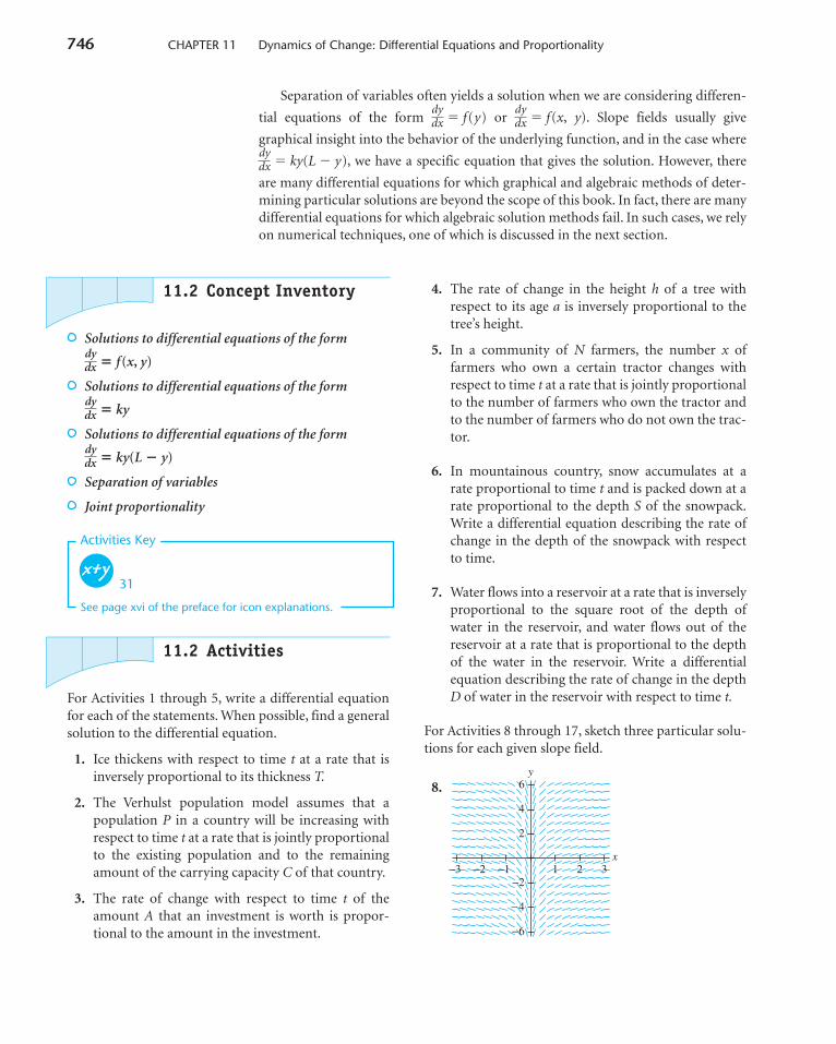
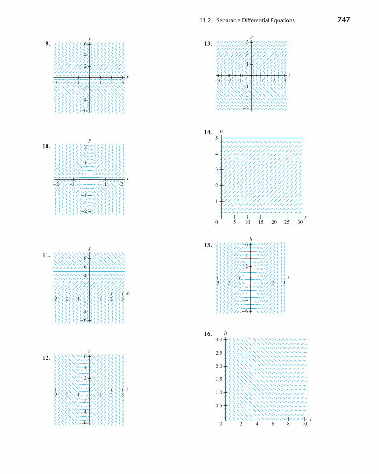
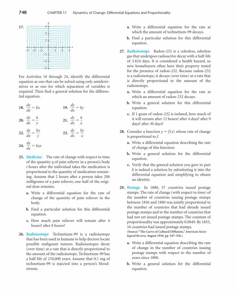
For Activities 8 through 17, sketch three particular solu-tions for each given slope field.

8.

x

y

321−3 −2 −1

−6

−4

−2

2

4

6

31

Activities Key

See page xvi of the preface for icon explanations.

4362_HMC_Ch11_722-764 12/23/03 7:53 PM Page 746


9.

10.

11.

12.g

321−3 −2 −1

−6

−4

−2

2

4

6

t

x

g

321−3 −2 −1

−6

−4

−2

2

4

6

8

x

y

1 2−2 −1

−2

−1

1

2

x

y

321−3 −2 −1

−6

−4

−2

2

4

6 13.

14.

15.

16.

0 108642t

h3.0

2.5

2.0

1.5

1.0

0.5

h

321−3 −2 −1

−6

−4

−2

2

4

6

t

5

4

3

2

1

0 30252015105x

h

t

g

321−3 −2 −1

−3

−2

−1

1

2

3

4362_HMC_Ch11_722-764 12/23/03 7:53 PM Page 747


17.

For Activities 18 through 24, identify the differentialequation as one that can be solved using only antideriv-atives or as one for which separation of variables isrequired. Then find a general solution for the differen-tial equation.

18. � kx 19. � ky

20. � 21. �

22. � 23. �

24. � kxy

25. Medicine The rate of change with respect to timeof the quantity q of pain reliever in a person’s bodyt hours after the individual takes the medication isproportional to the quantity of medication remain-ing. Assume that 2 hours after a person takes 200milligrams of a pain reliever, one-half of the origi-nal dose remains.

a. Write a differential equation for the rate ofchange of the quantity of pain reliever in thebody.

b. Find a particular solution for this differentialequation.

c. How much pain reliever will remain after 4hours? after 8 hours?

26. Radioisotope Technetium-99 is a radioisotopethat has been used in humans to help doctors locatepossible malignant tumors. Radioisotopes decay(over time) at a rate that is directly proportional tothe amount of the radioisotope. Technetium-99 hasa half-life of 210,000 years. Assume that 0.1 mg oftechnetium-99 is injected into a person’s blood-stream.

dydx

kyx

dydx

kxy

dydx

kx

dydx

ky

dydx

dydx

dydx

x

g

321−3 −2 −1

−3

−2

−1

1

2

3 a. Write a differential equation for the rate atwhich the amount of technetium-99 decays.

b. Find a particular solution for this differentialequation.

27. Radioisotope Radon-232 is a colorless, odorlessgas that undergoes radioactive decay with a half-lifeof 3.824 days. It is considered a health hazard, sonew homebuyers often have their property testedfor the presence of radon-232. Because radon-232is a radioisotope, it decays (over time) at a rate thatis directly proportional to the amount of theradioisotope.

a. Write a differential equation for the rate atwhich an amount of radon-232 decays.

b. Write a general solution for this differentialequation.

c. If 1 gram of radon-232 is isolated, how much ofit will remain after 12 hours? after 4 days? after 9days? after 30 days?

28. Consider a function y � f(x) whose rate of changeis proportional to f.




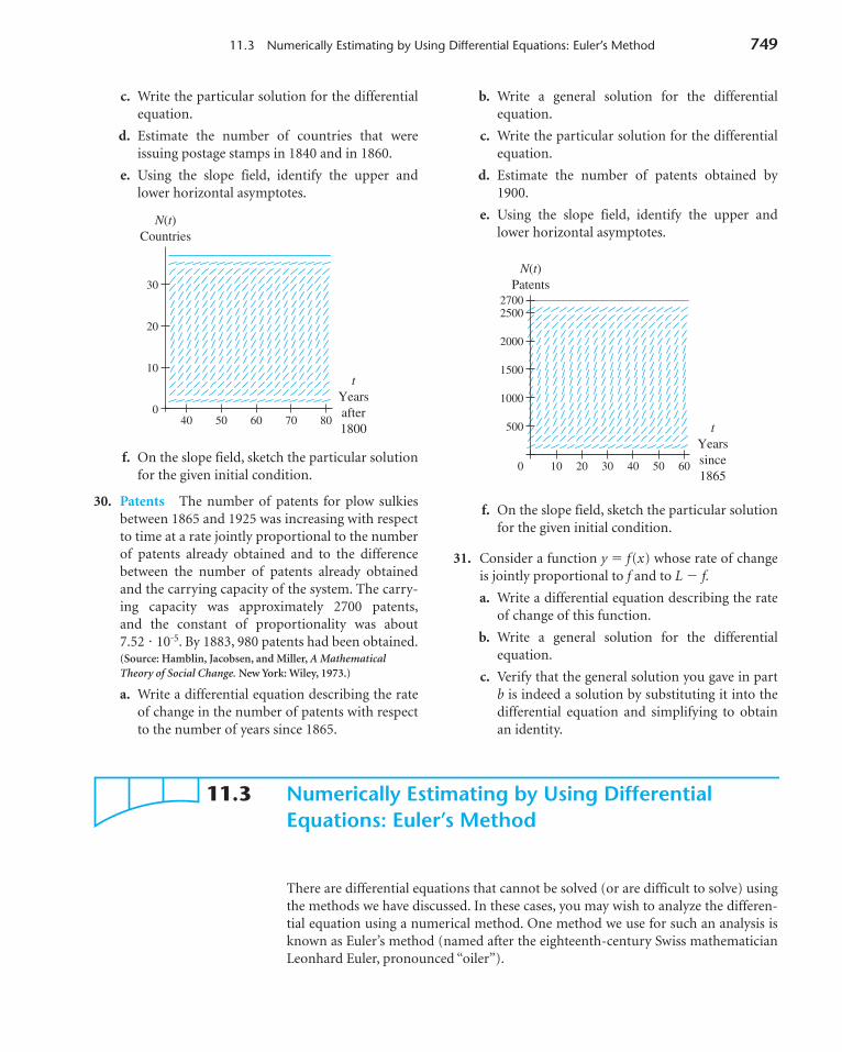
29. Postage In 1880, 37 countries issued postagestamps. The rate of change (with respect to time) ofthe number of countries issuing postage stampsbetween 1836 and 1880 was jointly proportional tothe number of countries that had already issuedpostage stamps and to the number of countries thathad not yet issued postage stamps. The constant ofproportionality was approximately 0.0049. By 1855,16 countries had issued postage stamps.(Source: “The Curve of Cultural Diffusion,” American Socio-logical Review, August 1936, pp. 547–556.)

a. Write a differential equation describing the rateof change in the number of countries issuingpostage stamps with respect to the number ofyears since 1800.


4362_HMC_Ch11_722-764 12/23/03 7:53 PM Page 748

11.3 Numerically Estimating by Using Differential Equations: Euler’s Method 749

c. Write the particular solution for the differentialequation.

d. Estimate the number of countries that wereissuing postage stamps in 1840 and in 1860.

e. Using the slope field, identify the upper andlower horizontal asymptotes.

f. On the slope field, sketch the particular solutionfor the given initial condition.

30. Patents The number of patents for plow sulkiesbetween 1865 and 1925 was increasing with respectto time at a rate jointly proportional to the numberof patents already obtained and to the differencebetween the number of patents already obtainedand the carrying capacity of the system. The carry-ing capacity was approximately 2700 patents,and the constant of proportionality was about 7.52 � 10�5. By 1883, 980 patents had been obtained.(Source: Hamblin, Jacobsen, and Miller, A Mathematical Theory of Social Change. New York: Wiley, 1973.)

a. Write a differential equation describing the rateof change in the number of patents with respectto the number of years since 1865.

N(t)

tYearsafter1800

Countries

80706050400

30

20

10


c. Write the particular solution for the differentialequation.

d. Estimate the number of patents obtained by1900.

e. Using the slope field, identify the upper andlower horizontal asymptotes.

f. On the slope field, sketch the particular solutionfor the given initial condition.

31. Consider a function y � f(x) whose rate of changeis jointly proportional to f and to L � f.




N(t)

tYearssince1865

Patents

50 6030 4010 200

2500

2000

1500

1000

500

2700

11.3 Numerically Estimating by Using Differential Equations: Euler’s Method

There are differential equations that cannot be solved (or are difficult to solve) usingthe methods we have discussed. In these cases, you may wish to analyze the differen-tial equation using a numerical method. One method we use for such an analysis isknown as Euler’s method (named after the eighteenth-century Swiss mathematicianLeonhard Euler, pronounced “oiler”).

4362_HMC_Ch11_722-764 12/23/03 7:53 PM Page 749


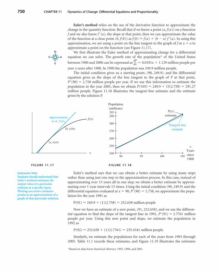
Euler’s method relies on the use of the derivative function to approximate thechange in the quantity function. Recall that if we know a point (a, f(a)) on a functionf and we also know f (a), the slope at that point, then we can approximate the valueof the function at a close point (b, f(b)) as f(b) � f(a) � (b � a) f (a). In using thisapproximation, we are using a point on the line tangent to the graph of f at x � a toapproximate a point on the function (see Figure 11.17).

We first illustrate the Euler method of approximating change for a differentialequation we can solve. The growth rate of the population* of the United States

between 1900 and 2000 can be expressed as � 0.0181x � 1.129 million people per

year x years after 1900. In 1990 the population was 249.9 million people.The initial condition gives us a starting point, (90, 249.9), and the differential

equation gives us the slope of the line tangent to the graph of P at that point,P(90) � 2.758 million people per year. If we use this information to estimate thepopulation in the year 2005, then we obtain P(105) � 249.9 � 15(2.758) � 291.27million people. Figure 11.18 illustrates the tangent-line estimate and the estimategiven by the solution P.


Euler’s method says that we can obtain a better estimate by using many stepsrather than using just one step in the approximation process. In this case, instead ofapproximating over 15 years all in one step, we obtain a better estimate by approxi-mating over 1-year intervals 15 times. Using the initial condition (90, 249.9) and thedifferential equation evaluated at x � 90, P(90) � 2.758, we approximate the popu-lation for the year 1991 as

P(91) � 249.9 � (1)(2.758) � 252.658 million people

Now we have an estimate of a new point, (91, 252.658), and we use the differen-tial equation to find the slope of the tangent line in 1991, P(91) � 2.7761 millionpeople per year. Using this new point and slope, we estimate the population in 1992 as

P(92) � 252.658 � (1)(2.7761) � 255.4341 million people

Similarly, we estimate the populations for each of the years from 1993 through2005. Table 11.1 records these estimates, and Figure 11.19 illustrates the estimates

Population(millions)

P(x)estimate

Tangent lineestimate

xYearssince1900

90 95 100 105

290

280

295

270

260

250

240x

f (x)

(a, f (a))

(b, f (b))

Approximationto (b, f (b))

dPdx


N

G A

V

*Based on data from Statistical Abstract, 1993, 1998, and 2001.

Instructor NoteStudents should understand thatEuler’s method estimates theoutput value of a particularsolution at a specific input.Plotting successive estimatesproduces an approximation of agraph of that particular solution.

4362_HMC_Ch11_722-764 12/23/03 7:53 PM Page 750


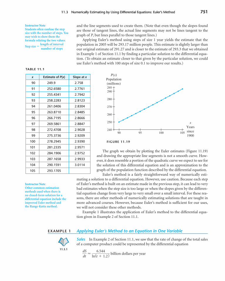
and the line segments used to create them. (Note that even though the slopes foundare those of tangent lines, the actual line segments may not be lines tangent to thegraph of P, but lines parallel to those tangent lines.)

Applying Euler’s method using steps of size 1 year yields the estimate that thepopulation in 2005 will be 293.17 million people. This estimate is slightly larger thanour original estimate of 291.27 and is closer to the estimate of 293.3 that we obtainedin Example 1 of Section 11.1 by finding a particular solution to the differential equa-tion. (To obtain an estimate closer to that given by the particular solution, we coulduse Euler’s method with 100 steps of size 0.1 to improve our results.)

The graph we obtain by plotting the Euler estimates (Figure 11.19)and drawing the appropriate line segments is not a smooth curve. How-ever, it does resemble a portion of the quadratic curve we expect to see forthe solution of this differential equation and is an approximation to thegraph of the population function described by the differential equation.

Euler’s method is a fairly straightforward way of numerically esti-mating a solution to a differential equation. However, use caution. Because each stepof Euler’s method is built on an estimate made in the previous step, it can lead to verybad estimates when the step size is too large or when the slopes given by the differen-tial equation change from very large to very small over a small interval. For these rea-sons, there are other methods of numerically estimating solutions that are taught inmore advanced courses. However, because Euler’s method is sufficient for our uses,we will not consider these other methods.

Example 1 illustrates the application of Euler’s method to the differential equa-tion given in Example 2 of Section 11.1.

EXAMPLE 1 Applying Euler’s Method to an Equation in One Variable

Sales In Example 2 of Section 11.1, we saw that the rate of change of the total salesof a computer product could be represented by the differential equation

� billion dollars per year6.544

ln(t � 1.2)dSdt


FIGURE 11.19

P(x)Population(millions)

xYearssince1900

90 95 100 105

290

280

295

270

260

250

240

Instructor NoteStudents often confuse the stepsize with the number of steps. Youmay wish to show them theformula relating the two values:

Step size �length of intervalnumber of steps

TABLE 11.1

x Estimate of P(x) Slope at x

90 249.9 2.758

91 252.6580 2.7761

92 255.4341 2.7942

93 258.2283 2.8123

94 261.0406 2.8304

95 263.8710 2.8485

96 266.7195 2.8666

97 269.5861 2.8847

98 272.4708 2.9028

99 275.3736 2.9209

100 278.2945 2.9390

101 281.2335 2.9571

102 284.1906 2.9752

103 287.1658 2.9933

104 290.1591 3.0114

105 293.1705

Instructor NoteOther common estimationmethods used when there is no closed-form solution for adifferential equation include theimproved Euler method and the Runge-Kutta method.

11.3.1

4362_HMC_Ch11_722-764 12/23/03 7:53 PM Page 751


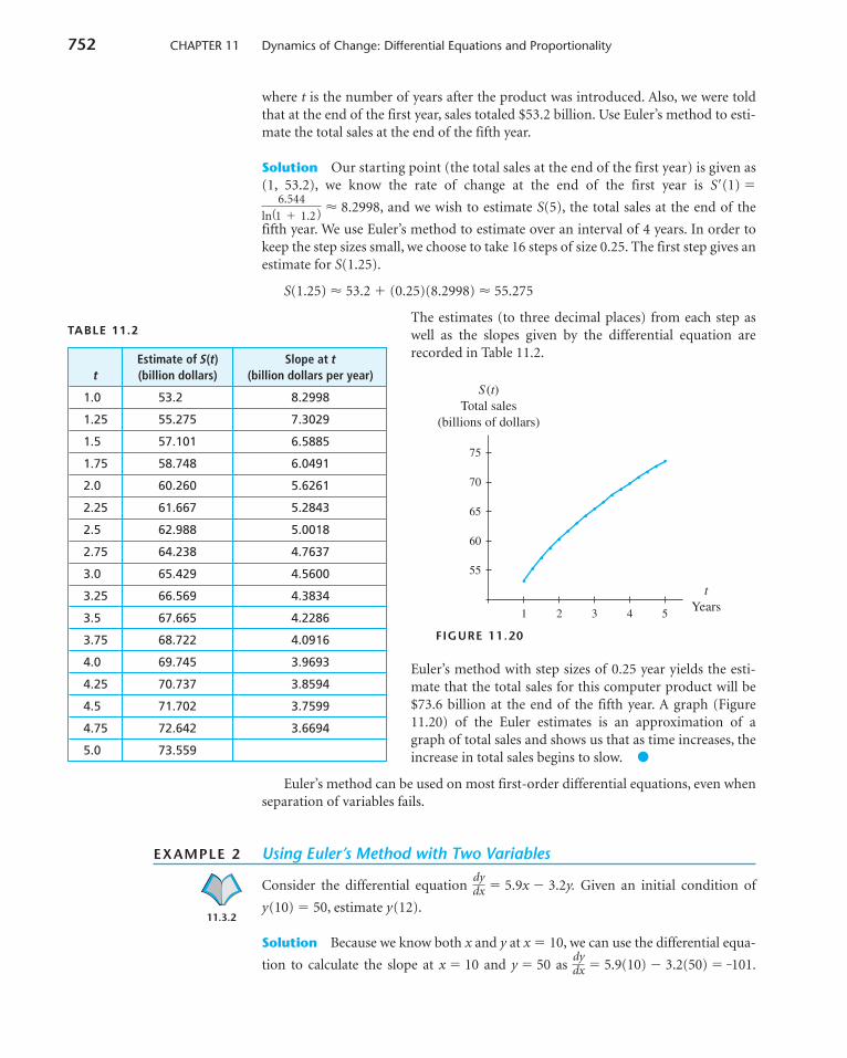
where t is the number of years after the product was introduced. Also, we were toldthat at the end of the first year, sales totaled $53.2 billion. Use Euler’s method to esti-mate the total sales at the end of the fifth year.

Solution Our starting point (the total sales at the end of the first year) is given as(1, 53.2), we know the rate of change at the end of the first year is S(1) �

� 8.2998, and we wish to estimate S(5), the total sales at the end of the

fifth year. We use Euler’s method to estimate over an interval of 4 years. In order tokeep the step sizes small, we choose to take 16 steps of size 0.25. The first step gives anestimate for S(1.25).

S(1.25) � 53.2 � (0.25)(8.2998) � 55.275

The estimates (to three decimal places) from each step aswell as the slopes given by the differential equation arerecorded in Table 11.2.

FIGURE 11.20

Euler’s method with step sizes of 0.25 year yields the esti-mate that the total sales for this computer product will be$73.6 billion at the end of the fifth year. A graph (Figure11.20) of the Euler estimates is an approximation of agraph of total sales and shows us that as time increases, theincrease in total sales begins to slow. ●

Euler’s method can be used on most first-order differential equations, even whenseparation of variables fails.

EXAMPLE 2 Using Euler’s Method with Two Variables

Consider the differential equation � 5.9x � 3.2y. Given an initial condition of

y(10) � 50, estimate y(12).

Solution Because we know both x and y at x � 10, we can use the differential equa-

tion to calculate the slope at x � 10 and y � 50 as � 5.9(10) � 3.2(50) � �101.dydx

dydx

tYears1 2 3 4 5

70

75

55

60

65

S (t)Total sales

(billions of dollars)

6.544

ln(1 � 1.2)

TABLE 11.2

Estimate of S(t) Slope at tt (billion dollars) (billion dollars per year)

1.0 53.2 8.2998

1.25 55.275 7.3029

1.5 57.101 6.5885

1.75 58.748 6.0491

2.0 60.260 5.6261

2.25 61.667 5.2843

2.5 62.988 5.0018

2.75 64.238 4.7637

3.0 65.429 4.5600

3.25 66.569 4.3834

3.5 67.665 4.2286

3.75 68.722 4.0916

4.0 69.745 3.9693

4.25 70.737 3.8594

4.5 71.702 3.7599

4.75 72.642 3.6694

5.0 73.559

11.3.2

4362_HMC_Ch11_722-764 12/23/03 7:53 PM Page 752


We choose to use Euler’s method with 10 steps of size 0.2. The first esti-mate is y(10.2) � 50 � (0.2)(�101) � 29.8.

Because the formula for the slope � 5.9x � 3.2y relies on

knowing both x and y to estimate the slope at x � 10.2, we must use ourestimate y(10.2) � 29.8 in the slope formula. Thus at x � 10.2,

� 5.9(10.2) � 3.2(29.8) � �35.18

We now use the estimates y(10.2) � 29.8 and � �35.18 at x � 10.2

to estimate the value of y at x � 10.4: y(10.4) � 29.8 � (0.2)(�35.18) �22.764.

To find an estimate of y(10.6), we need the slope at x � 10.4.

Again we must estimate this slope at x � 10.4 using y(10.4):

� 5.9(10.4) � 3.2(22.764) � �11.4848

Thus the value of y at x � 10.6 is

y(10.6) � 22.764 � (0.2)(�11.4848) � 20.46704

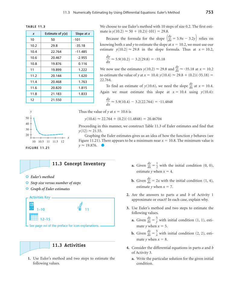
Proceeding in this manner, we construct Table 11.3 of Euler estimates and find thaty(12) � 21.55.

Graphing the Euler estimates gives us an idea of how the function y behaves (seeFigure 11.21). There appears to be a minimum near x � 10.8. The minimum value isy � 19.876. ●

dydx

dydx

dydx

dydx

�dydx�

FIGURE 11.21

x11

50

20

30

40

y

10 10.5 11.5 12

TABLE 11.3

x Estimate of y (x) Slope at x

10 50 �101

10.2 29.8 �35.18

10.4 22.764 �11.485

10.6 20.467 �2.955

10.8 19.876 0.116

11 19.899 1.222

11.2 20.144 1.620

11.4 20.468 1.763

11.6 20.820 1.815

11.8 21.183 1.833

12 21.550


Euler’s method

Step size versus number of steps

Graph of Euler estimates

11.3 Activities

1. Use Euler’s method and two steps to estimate thefollowing values.

a. Given � with the initial condition (0, 0),

estimate y when x � 4.

b. Given � 2x with the initial condition (1, 4),

estimate y when x � 7.

2. Are the answers to parts a and b of Activity 1approximate or exact? In each case, explain why.

3. Use Euler’s method and two steps to estimate thefollowing values.

a. Given � with initial condition (1, 1), esti-

mate y when x � 5.

b. Given � with initial condition (2, 2), esti-

mate y when x � 8.

4. Consider the differential equations in parts a and bof Activity 3.

a. Write the particular solution for the given initialcondition.

5x

dydx

5y

dydx

dydx

12

dydx

1–10 11

12–15

Activities Key


4362_HMC_Ch11_722-764 12/23/03 7:53 PM Page 753


b. Sketch the particular solution.

c. Sketch the Euler estimate.

d. Explain why the Euler estimate deviates fromthe true solution.

5. Weight For the first 9 months of life, the averageweight w, in pounds, of a certain breed of dogincreases at a rate that is inversely proportional totime t, in months. A 1-month old puppy weighs 6 pounds. The constant of proportionality is33.67885.

a. Write a differential equation describing the rateof change of the weight of the puppy.

b. Use Euler’s method with a 0.25-month steplength to estimate the weight of the puppy at 3 months and at 6 months.

c. Use Euler’s method with a step length of 1month to estimate the weight of the puppy at 3 months and at 6 months.

d. Do you expect the answer to part b or the answerto part c to be more accurate? Why?

6. Postage The rate of change (with respect totime) of the number of countries issuing postagestamps between 1836 and 1880 was jointly propor-tional to the number of countries that had alreadyissued postage stamps and to the number of coun-tries that had not yet issued postage stamps. Theconstant of proportionality was approximately0.0049. By 1855, 16 countries had issued postagestamps.(Source: “The Curve of Cultural Diffusion,” American Socio-logical Review, August 1936, pp. 547–556.)

a. Write a differential equation describing the rateof change in the number of countries issuingpostage stamps with respect to the number ofyears since 1800.

b. Use Euler’s method with 5 steps to estimate thenumber of countries issuing postage stamps in1840.

c. Use Euler’s method with a step length of 5 yearsto estimate the number of countries issuingpostage stamps in 1840.

d. Do you expect the answer to part b or the answerto part c to be more accurate? Why?

7. Production It is estimated that for the first 10years of production, a certain oil well can beexpected to produce oil at a rate of

r(t) � 3.935t 3.55e�1.35135t

thousand barrels per year

t years after production begins.

a. Write a differential equation for the rate ofchange of the total amount of oil produced tyears after production begins.

b. Use Euler’s method with 10 intervals to estimatethe yield from this oil well during the first 5years of production.

c. Graph the differential equation and the Eulerestimates. Discuss how the shape of the graph ofthe differential equation is related to the shapeof the graph of the Euler estimates.

8. Labor The personnel manager for a large con-struction company keeps records of the workerhours per week spent on typical construction jobshandled by the company. The manager has devel-oped the following model for a worker hours curve:

r(x) �

worker hours per week

the xth week of the construction job.

a. Use this model to write a differential equationgiving the rate of change of the total number ofworker hours used by the end of the xth week.

b. Graph this differential equation, and discuss anycritical points and trends that the differentialequation suggests will occur.

c. Use Euler’s method with 20 intervals to estimatethe total number of worker hours used by theend of the twentieth week.

d. Graph the Euler estimates, and discuss whetheryou believe the estimate is good. Refer to thepoints you discussed in part b. How could youimprove the accuracy of your estimate?

9. Cooling Newton’s Law of Cooling says that therate of change (with respect to time t) of the tem-perature T of an object is proportional to the differ-ence between the temperature of the object and thetemperature A of the object’s surroundings.

a. Write a differential equation describing this law.

6,608,830e�0.705989x

(1 � 925.466e�0.705989x)2

4362_HMC_Ch11_722-764 12/23/03 7:53 PM Page 754

11.4 Second-Order Differential Equations 755

b. Consider a room that has a constant tempera-ture of A � 70°F. An object is placed in thatroom and allowed to cool. When the object isfirst placed in the room, the temperature of theobject is 98°F, and it is cooling at a rate of 1.8°Fper minute. Determine the constant of propor-tionality for the differential equation.

c. Use Euler’s method and 15 steps to estimate thetemperature of the object after 15 minutes.

10. Learning A person learns a new task at a rate thatis equal to the percentage of the task not yetlearned. Let p represent the percentage of the taskalready learned at time t (in hours).

a. Write a differential equation describing the rateof change in the percentage of the task learned attime t.

b. Use Euler’s method with eight steps of size 0.25to estimate the percentage of the task that islearned in 2 hours.

c. Graph the Euler estimates, and discuss any criti-cal points or trends.

11. Explain why you would expect Euler’s method tohave better accuracy when more steps of smallersize are used. Illustrate with graphs.

12. Postage Refer to the information given in Activ-ity 6 about the rate of change of the number ofcountries issuing postage stamps.

a. Use Euler’s method with 40 steps and with 80steps to estimate the number of countries issu-ing postage stamps in 1840.

b. Graph the Euler estimates in part a.

c. Discuss your expectations for the accuracy ofyour answers.

13. Production Refer to the information given inActivity 7 about the rate of production of oil froman oil well.

a. Use Euler’s method with intervals of one month,then with intervals of one week, and finally withdaily intervals to estimate the yield from the wellduring the first 5 years of production.


c. Discuss your expectations for the accuracy ofyour answers.

14. Labor Refer to the information given in Activity8 about the manpower on a construction job.

a. Use Euler’s method with 140 intervals to esti-mate the total number of worker hours used bythe end of the twentieth week.


c. Discuss your expectations for the accuracy ofyour answers. Does an estimate using 140 inter-vals have any advantage over an estimate using20 intervals? Explain.

15. Cooling Refer to the information given in Activity 9 about Newton’s Law of Cooling. Con-sider especially the specification given in part b ofActivity 9.

a. Use Euler’s method with intervals of length onesecond to estimate the temperature of the objectafter 15 minutes.


c. How does this estimate compare with that foundin part c of Activity 9? Discuss the accuracy ofthis method.

11.4 Second-Order Differential Equations

Not all differential equations involve only the first derivative of a function. Some tellus about the second derivative. That is, they tell us about the rate at which the rate ofchange is changing.

Instructor NoteYou may wish to point out to yourstudents that this accelerationexample is essentially the same asExample 5 in Section 6.4.

4362_HMC_Ch11_722-764 12/23/03 7:53 PM Page 755


Because acceleration is the derivative of velocity v with respect to time t andvelocity is the derivative of distance s with respect to time, we can write accelerationdue to gravity near the surface of the Earth as the differential equation

� �32 feet per second squared

after t seconds. This differential equation is of the form s�(t) � k for some constant k.(We saw these equations in Chapter 6 when working with antiderivatives.) This is asecond derivative of a function, so a general solution can be found by finding the

general antiderivative of twice. The general antiderivative of the differential equa-

tion for acceleration is

� �32t � C feet per second

Thus the general solution to the differential equation is

s(t) � �16t2 � Ct � D feet

after t seconds.To confirm that this equation is a solution to the differential equation, we substi-

tute for s in the differential equation.

(�16t2 � Ct � D) � �32

Differentiating the left side of the equation twice yields the identity �32 � �32.In the case where the object fell from a height of 40 feet (s � 40 and v � 0 at

t � 0), we have the particular solution s(t) � �16t2 � 40 feet after t seconds.

EXAMPLE 1 Solving a Second-Order Linear Differential Equation

Purchasing Power The rate of change in the purchasing power* of the U.S. dollarwas changing at a linear rate between 1988 and 2000. A differential equation describ-ing the rate at which the rate of change of the purchasing power was decreasing is

� �0.00156x � 0.0115 dollars per year squared

where x is the number of years since 1988. The purchasing power is based on 1982dollars, making a 1982 dollar worth $0.93 in 1988 and $0.81 in 1992.

a. Write a general solution for the purchasing power of a dollar.

b. Write a particular solution for the purchasing power of a dollar.

c. Use the particular solution to determine how much a 1982 dollar was worth in2000.

d 2 Pdx2

d2

dt 2

dsdt

d2 sdt2

d2 sdt2

*Based on data from Statistical Abstract, 1994 and 2001.

4362_HMC_Ch11_722-764 12/23/03 7:53 PM Page 756


Solution

a. By finding the antiderivative of the differential equation twice, we obtain the gen-eral solution

P(x) � �0.00026x3 � 0.00575x2 � Cx � D dollars

where x is the number of years since 1988.

b. The conditions given are P(4) � 0.81 and P(0) � 0.93. The condition P(0) � 0.93 gives us the value for D as 0.93. Using D � 0.93 and P(4) � 0.81, wesolve for C and find that C � �0.0488. Thus we have the particular solution

P(x) � �0.00026x3 � 0.00575x2 � 0.0488x � 0.93 dollars

where x is the number of years since 1988.

c. By 2000, a 1982 dollar was worth only P(12) � $0.72. ●

Let us now consider situations in which the second derivative of an amount isproportional to the amount function; that is,

� ky

First we consider the case where the constant of proportionality is negative:

� �ky for k � 0

Consider the differential equation � �y. One function we have looked at

that satisfies this equation is the function y(x) � sin x. We verify this by differentia-ting the function twice:

y(x) � cos x

y�(x) � �sin x � �y(x)

The cosine function is another function that satisfies � �y.

For the more general case � �ky, where k � 0, it can be shown that the gen-

eral solution is

y(x) � a sin x � c

where a and c are constants. You will be asked to verify this in the activities.

EXAMPLE 2 Solving a Second-Order Differential Equation

Fishing An exclusive fishing club on the Restigouche River in Canada kept detailedrecords regarding the number of fish caught by its members.* Between 1880 and1905, the rate of change (with respect to the year) in the number of fish per rod perday was changing at a rate proportional to the number of fish per rod per day. Theconstant of proportionality is approximately �0.455625.

��k�

d2 y

dx2

d2 y

dx2

d2 y

dx2

d2ydx2

d2ydx2

Instructor NoteIf you did not cover Chapter 8, youmay want to omit this discussionand Example 2.

*Based on information in E. R. Dewey and E. F. Dakin, Cycles: The Science of Prediction (New York: Holt,1947).

4362_HMC_Ch11_722-764 12/23/03 7:53 PM Page 757


The average number of fish per rod per day for the years between 1880 and 1905was 1.267 fish per rod per day. In 1881, the catch was 0.9425 fish per rod per day, andin 1885, 1.5776 fish per rod per day were caught.

a. Write a differential equation expressing the rate at which the rate of change in thenumber of fish per rod per day was changing with respect to the number of yearssince 1880.

b. Write a particular solution to the differential equation.

c. Write a model for the average number of fish per rod per day given the number ofyears since 1880.

Solution

a. A differential equation expressing the rate at which the rate of change in g, thenumber of fish per rod per day, was changing is

� �0.455625g fish per rod per day per year squared

where y is the number of years since 1880.

b. As previously stated, the general solution is g(y) � a sin y � c where

k � 0.455625. Thus the general solution to this differential equation is

g(y) � a sin(0.675y � c) fish per rod per day

where y is the number of years since 1880, and a and c are constants. In order todetermine the constants a and c for this equation, we must have two conditions.First, we note that the general solution does not include the parameter d givingthe expected number of fish per rod per day that is normally included in a gen-eral sine model f(x) � a sin(bx � c) � d. Thus we must write the conditions interms of the difference from the expected value. That is, in 1881, the catch was0.3245 fewer fish per rod per day than in an average year, and in 1885, the catchwas 0.3106 more fish per rod per day than in an average year. Thus the two con-ditions are g(1) � �0.3245 and g(5) � 0.3106 resulting in the equations

�0.3245 � a sin[0.675(1) � c] (5)

0.3106 � a sin[0.675(5) � c] (6)

Solving for a in equation 5 and substituting in equation 6 yields

0.3106 �

which gives c � 1.019. Substituting this value of c into either equation 5 or equa-tion 6 and solving for a yields a � �0.327. Using these constants a and c, we havethe particular solution for the differential equation as

g(y) � �0.327 sin(0.675y � 1.019) fish per rod per day

where y is the number of years since 1880.

c. The general and particular solutions for the differential equation are both interms of the difference from the expected value of fish per rod per day. To write

�0.3245 sin(3.375 � c)sin(0.675 � c)

��k�

d 2 gdy 2

Instructor NoteShow your students the connectionbetween the two occurrences of theword rate in the statement in parta, “Write . . . the rate at which therate of change in . . . waschanging . . . with respect to thenumber of years,” and the use ofthe words per year squared in thestatement of the answer to part a.

4362_HMC_Ch11_722-764 12/23/03 7:53 PM Page 758


the general sine model for this situation, we add the parameter d, the expectedvalue of fish per day:

g(y) � �0.327 sin(0.675y � 1.019) � 1.267 fish per rod per day

where y is the number of years since 1880. ●

Before we leave this section, let us consider the differential equation of the form

� ky where k � 0

In this case, the constant of proportionality is positive (rather than negative as inExample 2) and the general solution is

y(x) � �

where a and b are constants. Note that the general solution to this differential equa-tion appears to be very different from the general solution in the negative case. Thenegative case leads to a model with which we are familiar; the positive case does not.

be��kxae�kx

d2 ydx2


Second-order differential equations


� k


� f (x)


� ky

11.4 Activities

For Activities 1 through 4, write a differential equationexpressing the information given and, when possible,find a general solution for the differential equation.

1. The Rowan-Robinson model of the universeassumes that the universe is expanding with respectto time t at a rate that is decreasing in inverse pro-portion to the square of its current size S.

d2ydx2

d2ydx2

d2ydx2

2. The rate of change with respect to time t of thedemand D for a product is decreasing proportion-ately to the demand at time t.

3. The rate of change in year y of the population P ofthe United States is increasing with respect to theyear at a constant rate.

4. The rate of growth of the height h of a young childwith respect to the age y of the child decreases ininverse proportion to the age of the child.

5. Jobs The rate of change in the number of jobs fora Michigan roofing company is increasing byapproximately 6.14 jobs per month squared. Thenumber of jobs in January is decreasing at the rateof 0.87 job per month, and company records indi-cate that the company had 14 roofing jobs in February.

a. Write a differential equation for the rate atwhich the rate of change in the number of roof-ing jobs for this company is changing.

b. Find a particular solution to the differentialequation in part a.

c. Use the result of part b to estimate the numberof roofing jobs in August and the number inNovember.

6. Marriage Between 1950 and 2000, the rate ofchange in the rate at which the median age of firstmarriage of females in the United States was chang-ing was constant at 0.0042 year of age per year

5–11 12

Activities Key


4362_HMC_Ch11_722-764 12/23/03 7:53 PM Page 759


squared. The median age of first marriage for thesefemales was increasing at the rate of 0.1713 year ofage per year in 1991, and females were first marriedat a median age of 25.1 in 2000.(Source: Based on data from www.infoplease.com. Accessed9/20/02.)

a. Write a differential equation for the rate atwhich the rate of the median age of first mar-riage for United States females is changing.


c. Use the result of part b to estimate the medianage of first marriage of United States females inthe current year.

7. AIDS Records of the number of AIDS cases diag-nosed in the United States between 1988 and 1991indicate that the rate at which the rate of change inthe number of cases was changing was constant at�2099 cases per year squared. The number of AIDScases diagnosed in 1988 was 33,590, and the num-ber of cases was increasing at the rate of 5988.7cases per year in 1988.(Source: Based on data appearing in the HIV/AIDS Surveil-lance 1992 Year End Edition.)

a. Write a differential equation for the rate ofchange of the rate of change of the number ofAIDS cases diagnosed in year t, where t is thenumber of years after 1988.


c. Estimate how rapidly the number of AIDS casesdiagnosed was changing in 1991 and the num-ber of AIDS cases that was diagnosed in thatyear.

8. Postage Between 1919 and 1995, the rate ofchange of the rate of change of the postage requiredto mail a first-class 1-ounce letter was approxi-mately 0.022 cent per year squared. The postagewas 2 cents in 1919, and it was increasing at the rateof approximately 0.393 cent per year in 1958.(Source: Based on data from the United States Postal Service.)

a. Write a differential equation for the rate ofchange of the rate of change of the first-classpostage for a 1-ounce letter in year t, where t isthe number of years after 1900.

b. Find both a general and a particular solution tothe differential equation in part a.

c. Use your previous results to estimate how rap-idly the postage is changing in the current yearand the current first-class postage for a 1-ounceletter. Comment on the accuracy of your results.If they are not reasonable, give possible explana-tions.

9. Consider a function y � f(x) whose rate of changewith respect to x is changing at a constant rate.

a. Write a differential equation describing the rateof change in the rate of change for this function.



10. Motion Laws When a spring is stretched andthen released, it oscillates according to two laws ofphysics: Hooke’s Law and Newton’s Second Law.These two laws combine to form the following dif-ferential equation in the case of free, undampedoscillation:

m � kx � 0

where m is the mass of an object attached to thespring, x is the distance the spring is stretchedbeyond its standard length with the object attached(its equilibrium point), t is time, and k is a constantassociated with the strength of the spring. Considera spring with k � 15 from which is hung a 30-pound weight. The spring with the weight attachedstretches to its equilibrium point. The spring isthen pulled 2 feet farther than its equilibrium andreleased.

a. Write a differential equation describing theacceleration of the spring with respect to time tmeasured in seconds. Use the fact that

mass � where g is the gravitational

constant 32 feet per second per second.

b. Write a particular solution for this differentialequation. Use the fact that when the spring isfirst released, its velocity is 0.

weightg

d2xdt 2

4362_HMC_Ch11_722-764 12/23/03 7:53 PM Page 760

11.4 Summary 761

c. Graph this solution over several periods, andexplain how to interpret the graph.

d. How quickly is the mass moving when it passesits equilibrium point?

11. Radiation The rate of change in the rate at whichthe average amount of extraterrestrial radiation inAmarillo, Texas, for each month of the year ischanging is proportional to the amount of extrater-restrial radiation received. The constant of propor-tionality is k � � 0.212531. In any given month, theexpected value of radiation is 12.5 mm per day.This expected value is actually obtained in Marchand September.(Source: Based on data from A. A. Hanson, ed., Practical Hand-book of Agricultural Science. Boca Raton, FL: CRC Press, 1990.)

a. Write a differential equation for the informationgiven.

b. In June, the amount of radiation received isapproximately 17.0 mm per day, and in Decem-

ber, the amount of radiation received is approxi-mately 7.8 mm per day. Write a particular solution for this differential equation.

c. Change the particular solution into a functiongiving the average amount of extraterrestrialradiation in Amarillo.

d. How well does your model estimate theamounts of extraterrestrial radiation in Marchand September?

12. Consider a function y � f(x) whose rate of changewith respect to x is changing in proportion to fwhere the constant of proportionality is negative.

a. Write a differential equation describing the rateof change in the rate of change for this function.


c. Verify that the general solution you gave in partb is indeed a solution by substituting it into thedifferential equation and obtaining an identity.

In many situations (physical, sociological, psychologi-cal, and economic), there are certain laws that govern

the dynamics of change. In these cases, differentialequations often can be used to describe the change thatoccurs.

Differential Equations

Differential equations are equations involving deriva-tives. A solution for a differential equation is a functionthat, when substituted into the differential equation,results in an identity. A general solution contains arbi-trary constants that can be determined if initial condi-tions are known. When the arbitrary constants arereplaced by known constants, the solution is called aparticular solution.

Some differential equations are of the simple form

� f(x)

In this case, a general solution can be obtained by writ-ing a general antiderivative for the given rate of changeif an antiderivative is known.

Slope Fields

It is often helpful to view a graphical representation of adifferential equation. This can be done in the form of aslope field. A slope field consists of line segments thatrepresent the slopes given by the differential equation atdifferent points on a grid placed on the coordinateplane.

dydx

SUMMARY

4362_HMC_Ch11_722-764 12/23/03 7:53 PM Page 761


Separable Differential Equations

Some differential equations are given as functions notonly of the input variable but also of the output vari-able, so they are of the form

� f(x, y)

In this case, a general solution might be obtained byusing the method of separation of variables.

Euler’s Method

Often, neither simple antidifferentiation nor separationof variables is sufficient for determining an explicit for-

dydx

mula for a general solution of a differential equation. Inthese cases, we can numerically estimate a solutionusing Euler’s method. Euler’s method not only gives us anumerical method for estimating solutions but also,when the Euler estimates are graphed, can help us visu-alize how the solution function behaves.

Second-Order Differential Equations

Second-order differential equations involve the secondderivative of a function. The simple cases we consideredwere the second-order differential equations that giverise to the quadratic, cubic, and sine models.

CONCEPT CHECK

Can you

Solve constant and linear differential equations?Set up an equation involving direct or inverse pro-portionality?Sketch a particular solution to a differential equa-tion on a slope field?Solve separable differential equations?Set up an equation involving joint proportionality?Estimate a solution to a differential equation usingEuler’s method?Set up and solve second-order differential equa-tions using antiderivatives?

To practice, try

Section 11.1 Activities 15, 19

Section 11.1 Activities 19, 23Section 11.1 Activities 7, 9Section 11.2 Activities 9, 13, 15Section 11.2 Activity 25Section 11.2 Activity 29

Section 11.3 Activity 7

Section 11.4 Activities 7, 11

Instructor NoteThe Concept Check provides students a quick way of checking on which topics they need to spendmore time. The activities listed here are generally simple ones, and the students should be warned that being able to do these activities does not guarantee that they fully understand all the concepts—especially not if they only read through the activity and look at the answer in the back of the bookwithout actually working through the solution themselves.CONCEPT CHECK

4362_HMC_Ch11_722-764 12/23/03 7:53 PM Page 762

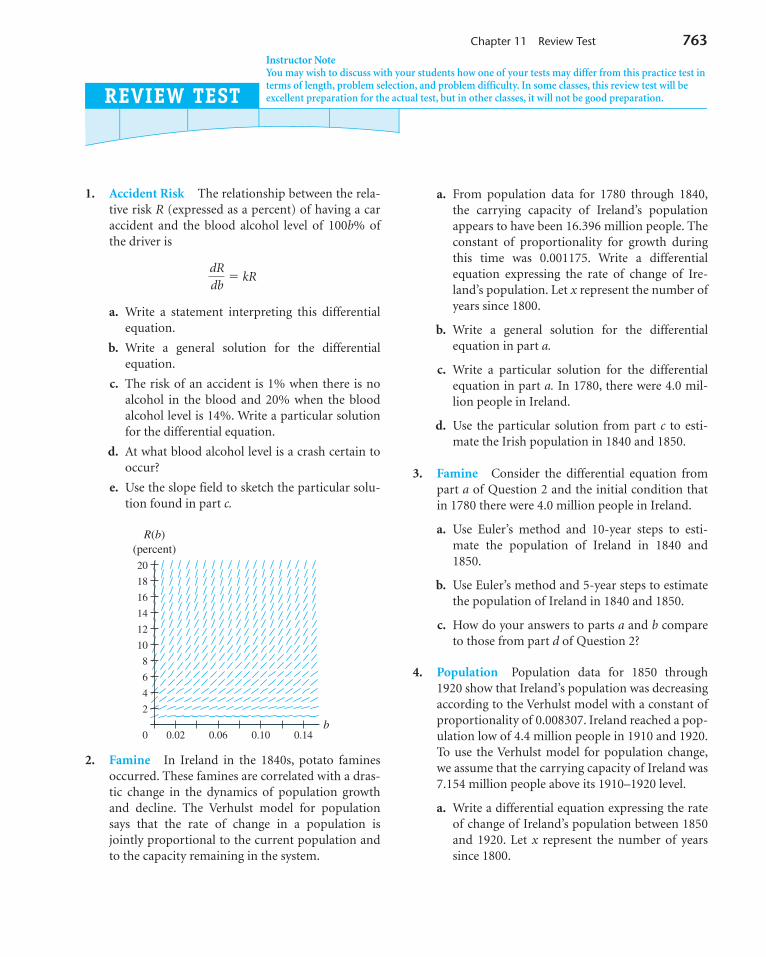
Chapter 11 Review Test 763Instructor NoteYou may wish to discuss with your students how one of your tests may differ from this practice test interms of length, problem selection, and problem difficulty. In some classes, this review test will beexcellent preparation for the actual test, but in other classes, it will not be good preparation.REVIEW TEST

1. Accident Risk The relationship between the rela-tive risk R (expressed as a percent) of having a caraccident and the blood alcohol level of 100b% ofthe driver is

� kR

a. Write a statement interpreting this differentialequation.


c. The risk of an accident is 1% when there is noalcohol in the blood and 20% when the bloodalcohol level is 14%. Write a particular solutionfor the differential equation.

d. At what blood alcohol level is a crash certain tooccur?

e. Use the slope field to sketch the particular solu-tion found in part c.

2. Famine In Ireland in the 1840s, potato faminesoccurred. These famines are correlated with a dras-tic change in the dynamics of population growthand decline. The Verhulst model for populationsays that the rate of change in a population isjointly proportional to the current population andto the capacity remaining in the system.

4

8

12

16

20

2

6

10

14

18

0 0.140.100.02 0.06b

R(b)(percent)

dRdb

a. From population data for 1780 through 1840,the carrying capacity of Ireland’s populationappears to have been 16.396 million people. Theconstant of proportionality for growth duringthis time was 0.001175. Write a differentialequation expressing the rate of change of Ire-land’s population. Let x represent the number ofyears since 1800.

b. Write a general solution for the differentialequation in part a.

c. Write a particular solution for the differentialequation in part a. In 1780, there were 4.0 mil-lion people in Ireland.

d. Use the particular solution from part c to esti-mate the Irish population in 1840 and 1850.

3. Famine Consider the differential equation frompart a of Question 2 and the initial condition thatin 1780 there were 4.0 million people in Ireland.

a. Use Euler’s method and 10-year steps to esti-mate the population of Ireland in 1840 and1850.

b. Use Euler’s method and 5-year steps to estimatethe population of Ireland in 1840 and 1850.

c. How do your answers to parts a and b compareto those from part d of Question 2?

4. Population Population data for 1850 through1920 show that Ireland’s population was decreasingaccording to the Verhulst model with a constant ofproportionality of 0.008307. Ireland reached a pop-ulation low of 4.4 million people in 1910 and 1920.To use the Verhulst model for population change,we assume that the carrying capacity of Ireland was7.154 million people above its 1910–1920 level.

a. Write a differential equation expressing the rateof change of Ireland’s population between 1850and 1920. Let x represent the number of yearssince 1800.

4362_HMC_Ch11_722-764 12/23/03 7:53 PM Page 763


b. Using the fact that in 1900, there were 4.5 mil-lion people in Ireland (that is 0.1 million peopleabove its 1910–1920 level), write a particularsolution to the differential equation from part a.

c. Adjust the model for 1850 through 1920 byadding the base population level of 4.4 million

people, and write a piecewise model for the pop-ulation of Ireland from 1780 through 1920.

d. Use the piecewise model from part c to estimatethe population of Ireland in 1850. How does thisdiffer from the estimate you found in part d ofQuestion 2?

4362_HMC_Ch11_722-764 12/23/03 7:53 PM Page 764

Documents

11 Differential Equations and Proportionality - Cengagecollege.cengage.com/.../3e/students/ch11/401288_ch_11_722_764.pdf · CHAPTER Dynamics of Change: Differential Equations and