11-Borello Electrohydraulic Servovalves

7/17/2019 11-Borello Electrohydraulic Servovalves

http://slidepdf.com/reader/full/11-borello-electrohydraulic-servovalves 1/12

Annual Conference of the Prognostics and Health Management Society, 2009

A Prognostic Model for Electrohydraulic Servovalves

Lorenzo Borello1, Matteo Dalla Vedova

2, Giovanni Jacazio

3, Massimo Sorli

4

1,2 Politecnico of Turin - Department of Aerospace Engineering, Torino, [email protected]

[email protected]

3,4 Politecnico of Turin - Department of Mechanics, Torino, Italy [email protected]

[email protected]

ABSTRACT

Servovalves are critical components of the

hydraulic servos and their correct operation ismandatory to ensure the proper functioning of thecontrolled servosystem. A continuous monitor istypically performed that can detect a servovalveloss of operation, but falls short of recognizingother malfunctionings. A research was performedaimed at developing a prognostic algorithm ableto identity the precursors of a servovalve failureand its degradation pattern. A model basedtechnique was used that fuses several informationobtained by comparing actual with expectedresponse of the servovalve to recognize adegradation. The research was focused to flightcontrol systems, but it can be used in other

application areas. To assess the robustness of thealgorithm a simulation test environment wasdeveloped. Simulations were run in which aservovalve controlled actuator was subjected tosequences of commands and loads representativeof those encountered during actual operation, andvariations of the servovalve characteristics withintheir normal range were applied. At the sametime, degradations of the servovalve weresuperimposed and the merit of the prognosticsalgorithm was verified. The results showed anadequate robustness and confidence was gained inthe ability to detect servovalve degradations withlow risk of false alarms or missed failures.*

* Lorenzo Borello et al.: This is an open-access article distributed under

the terms of the Creative Commons Attribution 3.0 United States

License, which permits unrestricted use, distribution, and reproduction inany medium, provided the original author and source are credited.

1 FLOW CONTROL VALVES FOR FLIGHT

CONTROL SYSTEMS

Flight control systems of many civil and military

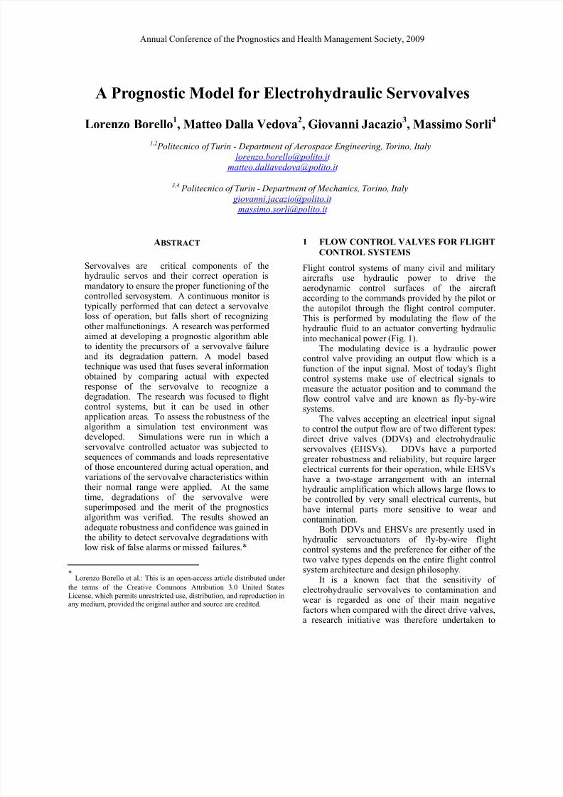
aircrafts use hydraulic power to drive theaerodynamic control surfaces of the aircraftaccording to the commands provided by the pilot orthe autopilot through the flight control computer.This is performed by modulating the flow of thehydraulic fluid to an actuator converting hydraulicinto mechanical power (Fig. 1).

The modulating device is a hydraulic powercontrol valve providing an output flow which is afunction of the input signal. Most of today's flightcontrol systems make use of electrical signals tomeasure the actuator position and to command theflow control valve and are known as fly-by-wiresystems.

The valves accepting an electrical input signalto control the output flow are of two different types:direct drive valves (DDVs) and electrohydraulicservovalves (EHSVs). DDVs have a purportedgreater robustness and reliability, but require largerelectrical currents for their operation, while EHSVshave a two-stage arrangement with an internalhydraulic amplification which allows large flows to

be controlled by very small electrical currents, buthave internal parts more sensitive to wear andcontamination.

Both DDVs and EHSVs are presently used inhydraulic servoactuators of fly-by-wire flightcontrol systems and the preference for either of the

two valve types depends on the entire flight controlsystem architecture and design philosophy.

It is a known fact that the sensitivity ofelectrohydraulic servovalves to contamination andwear is regarded as one of their main negativefactors when compared with the direct drive valves,a research initiative was therefore undertaken to




2

develop a prognostics model able to recognize a progressive deterioration of the servovalve characteristics,thereby alerting of a trend toward an unacceptableservovalve behaviour or a failure. A valid and reliable

prognostics model for the EHSVs could partly offset theweak points of these components, which on the other handoffer the merits of lower weight, much lower electrical

power consumption, greater chip shear capability andlower cost when compared with DDVs.

2

SERVOVALVE CONFIGURATIONS

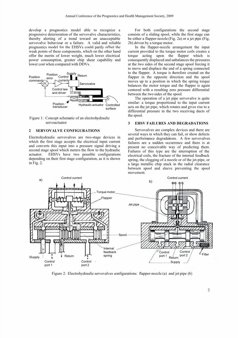
Electrohydraulic servovalves are two-stage devices inwhich the first stage accepts the electrical input currentand converts this input into a pressure signal driving asecond stage spool which meters the flow to the hydraulicactuator. EHSVs have two possible configurationsdepending on their first stage configuration, as it is shownin Fig. 2.

For both configurations the second stageconsists of a sliding spool, while the first stage can

be either a flapper-nozzle (Fig. 2a) or a jet pipe (Fig.2b) driven by a torque motor.

In the flapper-nozzle arrangement the inputcurrent provided to the torque motor coils creates atorque acting upon the flapper which is

consequently displaced and unbalances the pressuresat the two sides of the second stage spool forcing itto move and displace the end of a spring connectedto the flapper. A torque is therefore created on theflapper in the opposite direction and the spoolmoves up to a position in which the spring torque

balances the motor torque and the flapper is againcentered with a resulting zero pressure differential

between the two sides of the spool.The operation of a jet pipe servovalve is quite

similar: a torque proportional to the input currentacts on the jet pipe, which rotates and gives rise to adifferential pressure in the two receiving ducts ofthe spool.

3 EHSV FAILURES AND DEGRADATIONS

Servovalves are complex devices and there areseveral ways in which they can fail, or show defectsand performance degradations. A few servovalvesfailures are a sudden occurrence and there is at

present no conceivable way of predicting them.Failures of this type are the interruption of theelectrical coils, the fracture of the internal feedbackspring, the clogging of a nozzle or of the jet-pipe, ora large metallic chip stuck in the radial clearance

between spool and sleeve preventing the spoolmovement.

Control current Control current

Torque motor

Flapper

Jet pipe

Supply

Supply

Return

Controlport 1

Controlport 2

Controlport 1

Controlport 2

Return

Internalfeedbackspring

Spool

Filter

a) b)

Figure 2: Electrohydraulic servovalves configurations: flapper-nozzle (a) and jet pipe (b)

Positioncommand

Positionerror Control

currentServovalve

Positiontransducer

Hydraulic actuator Controlledsurface

Supply Return

Control lawand driver

Figure 1: Concept schematic of an electrohydraulicservoactuator




3

All these failures are normally sudden unpredictableevents leading to a servovalve lack of operation, oruncommanded movement that are recognized by adedicated monitoring logic which eventually issues anappropriate command to a shutoff valve upstream of theservovalve, thereby removing the hydraulic power supplyfrom the servovalve and inhibiting any further operation.

In general, the servovalves are provided with anLVDT type position transducer that senses the spool

position; by comparing the servovalve current with thespool position a lack of response or an uncommandedmovement can be detected. There are however severalother scenarios in which a progressive degradation of aservovalve occurs, which does not initially create anunacceptable behaviour, but, if undetected, may lead to acondition in which the servovalve, and hence the wholeservoactuator operation is impaired.

Some along the possible progressive degradations of aservovalve are the following:1. Increased contamination of the first stage filter

(shown only in Fig. 2b, but always present also in the

flapper-nozzle servovalves). As dirt and debrisaccumulate in the first stage filter, its hydraulicresistance increases with a consequent reduction ofthe supply pressure available at the first stage andhence the pressure differential applicable to thespool. This results in a slower response of theservovalve, with increased phase lag and reduction ofthe servoactuator stability margin.

2. Reduction of the torque sensitivity of the first stagetorque motor. This can be the result of a shorting ofsome adjacent coils of the torque motor due to the

presence of metallic debris, or to a degradation of themagnetic properties of the materials. As for theabove case, a progressively slower response of theservovalve is obtained.

3. Increase in the backlash at the mechanical interface between the internal feedback spring and the secondstage spool. This is the result of a wear due to therelative movement between these two parts and givesrise to an increasing hysteresis in the servovalveresponse which leads to an instability of the wholehydraulic servoloop.

4. Increase in the friction force between spool andsleeve. This is due to a silting effect associated eitherto debris entrained by the hydraulic fluid or to thedecay of the hydraulic fluid additives which tend to

polymerize when the fluid is subjected to large shearstresses as they occur in the flows through smallclearances.

5. Increase in the radial clearance between spool andsleeve and change of the shape of the corners of thespool lands due to wear between these two moving

parts.The objective of the prognostic model is to put

together different pieces of information to recognize that aservovalve degradation is under way and predict theremaining useful life before its behaviour becomes

unacceptable and such to lead to an undesirableshutdown while in flight. It must be emphasized thatthe main purpose of the prognostics model is todetect a progressive degradation and estimate theremaining time to failure, while it does notspecifically indicate which is the cause of thedegradation, which can be positively assessed only

after disassembling the servovalve.

4 PHYSICAL MODEL OF AN EHSV

The authors have developed mathematicalmodels of hydraulic servosystems in which EHSVsor DDVs were controlling the flow delivered toeither a linear hydraulic actuator or to a hydraulicmotor. Models of different complexity andaccuracy were built, depending on the requiredaccuracy level. Examples of mathematical modelsdeveloped by the authors for hydraulic servosystemsare those for the AMX stabilizer actuation system(two torque summed hydraulic motors, EHSV

controlled), the C27J elevator and rudderservoactuators (hydro-mechanical servoloops), theEurofighter leading edge flap actuation system (twotorque summed hydraulic motors, DDV controlled),the M346 leading edge flap actuation system (twotorque summed hydraulic motors, EHSVcontrolled), the force control systems of the M346iron bird (linear hydraulic actuators with EHSVcontrol).

All these models were "physical-based" modelsin which all the system components were modelledwith equations representative of their physicalcharacteristics. The comparison between thesimulations and the test results allowed to

progressively tune the mathematical model whicheventually reached a good fidelity in representingthe actual system behaviour.

The proven fidelity of the mathematical modelsof hydraulic servos that were developed for theanalysis of the above mentioned systems providedus the necessary confidence to use a similarmathematical model for predicting the behaviour ofa hydraulic servo over the whole range of normaland degraded conditions without performingexpensive and time consuming tests. The model isvery detailed and describes the physical behaviourof each part of the servovalve.

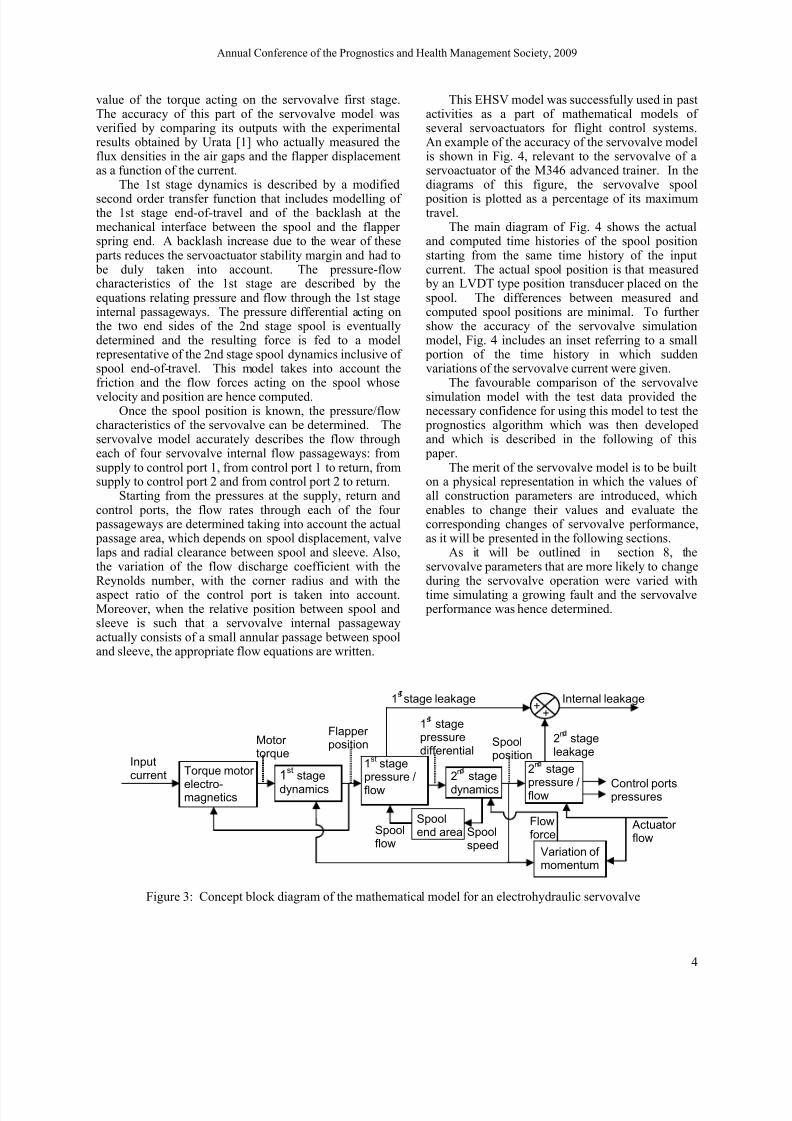
A concept block diagram of the servovalve

model is shown in Fig. 3. This block diagramspecifically refers to a flapper-nozzle servovalve,

but it can as well be applied to a jet pipe servovalve.The servovalve mathematical model accepts the

input current and works out the torque developed bythe torque motor according to the equationsdescribing in details its electromagnetics. Themodel computes the fluxes through the air gaps andhow they are modified by the electrical currentthrough the coils, and eventually determines the




4

value of the torque acting on the servovalve first stage.The accuracy of this part of the servovalve model wasverified by comparing its outputs with the experimentalresults obtained by Urata [1] who actually measured theflux densities in the air gaps and the flapper displacementas a function of the current.

The 1st stage dynamics is described by a modified

second order transfer function that includes modelling ofthe 1st stage end-of-travel and of the backlash at themechanical interface between the spool and the flapperspring end. A backlash increase due to the wear of these

parts reduces the servoactuator stability margin and had to be duly taken into account. The pressure-flowcharacteristics of the 1st stage are described by theequations relating pressure and flow through the 1st stageinternal passageways. The pressure differential acting onthe two end sides of the 2nd stage spool is eventuallydetermined and the resulting force is fed to a modelrepresentative of the 2nd stage spool dynamics inclusive ofspool end-of-travel. This model takes into account thefriction and the flow forces acting on the spool whose

velocity and position are hence computed.Once the spool position is known, the pressure/flow

characteristics of the servovalve can be determined. Theservovalve model accurately describes the flow througheach of four servovalve internal flow passageways: fromsupply to control port 1, from control port 1 to return, fromsupply to control port 2 and from control port 2 to return.

Starting from the pressures at the supply, return andcontrol ports, the flow rates through each of the four

passageways are determined taking into account the actual passage area, which depends on spool displacement, valvelaps and radial clearance between spool and sleeve. Also,the variation of the flow discharge coefficient with theReynolds number, with the corner radius and with theaspect ratio of the control port is taken into account.Moreover, when the relative position between spool andsleeve is such that a servovalve internal passagewayactually consists of a small annular passage between spooland sleeve, the appropriate flow equations are written.

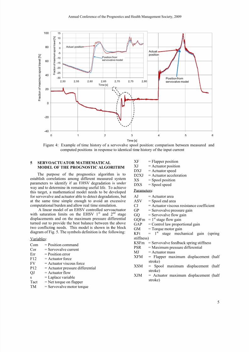
This EHSV model was successfully used in pastactivities as a part of mathematical models ofseveral servoactuators for flight control systems.An example of the accuracy of the servovalve modelis shown in Fig. 4, relevant to the servovalve of aservoactuator of the M346 advanced trainer. In thediagrams of this figure, the servovalve spool

position is plotted as a percentage of its maximumtravel.

The main diagram of Fig. 4 shows the actualand computed time histories of the spool positionstarting from the same time history of the inputcurrent. The actual spool position is that measured

by an LVDT type position transducer placed on thespool. The differences between measured andcomputed spool positions are minimal. To furthershow the accuracy of the servovalve simulationmodel, Fig. 4 includes an inset referring to a small

portion of the time history in which suddenvariations of the servovalve current were given.

The favourable comparison of the servovalve

simulation model with the test data provided thenecessary confidence for using this model to test the

prognostics algorithm which was then developedand which is described in the following of this

paper.The merit of the servovalve model is to be built

on a physical representation in which the values ofall construction parameters are introduced, whichenables to change their values and evaluate thecorresponding changes of servovalve performance,as it will be presented in the following sections.

As it will be outlined in section 8, theservovalve parameters that are more likely to changeduring the servovalve operation were varied withtime simulating a growing fault and the servovalve

performance was hence determined.

Inputcurrent Torque motor

electro-magnetics

Motor torque

1st stage

dynamics

1st stage

pressure /flow

Flapperposition

2n

stage

pressure /flow

2n

stage

dynamics

1s stage

pressuredifferential

Spoolposition

Spoolflow

Control portspressures

Actuatorflow

Variation ofmomentum

2n

stageleakage

Spoolend area Spool

speed

1sstage leakage

++

Internal leakage

Flowforce

Figure 3: Concept block diagram of the mathematical model for an electrohydraulic servovalve




5

5 SERVOACTUATOR MATHEMATICAL

MODEL OF THE PROGNOSTIC ALGORITHM

The purpose of the prognostics algorithm is toestablish correlations among different measured system

parameters to identify if an EHSV degradation is underway and to determine its remaining useful life. To achievethis target, a mathematical model needs to be developedfor servovalve and actuator able to detect degradations, butat the same time simple enough to avoid an excessivecomputational burden and allow real time simulation.

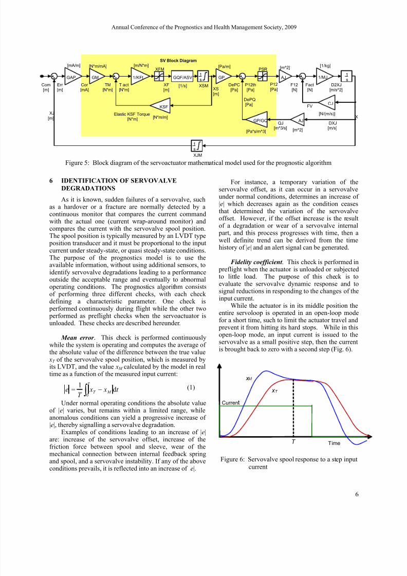
A linear model of an EHSV controlled servoactuatorwith saturation limits on the EHSV 1st and 2nd stagedisplacements and on the maximum pressure differentialturned out to provide the best balance between the abovetwo conflicting needs. This model is shown in the blockdiagram of Fig. 5. The symbols definition is the following:

Variables:

Com = Position commandCor = Servovalve current

Err = Position errorF12 = Actuator force

FV = Actuator viscous force

P12 = Actuator pressure differentialQJ = Actuator flow

s = Laplace variable

Tact = Net torque on flapper

TM = Servovalve motor torque

XF = Flapper position

XJ = Actuator position

DXJ = Actuator speedD2XJ = Actuator acceleration

XS = Spool position

DXS = Spool speedParameters:

AJ = Actuator areaASV = Spool end area

CJ = Actuator viscous resistance coefficient

GP = Servovalve pressure gainGQ = Servovalve flow gain

GQFm = 1st stage flow gain

GAP = Control law proportional gain

GM = Torque motor gainKFt = 1st stage mechanical gain (spring

stiffness)

KSFm = Servovalve feedback spring stiffness

PSR = Maximum pressure differentialMJ = Actuator massXFM = Flapper maximum displacement (half

stroke)

XSM = Spool maximum displacement (halfstroke)

XJM = Actuator maximum displacement (half

stroke)

-40

-20

0

20

40

60

80

100

0 1 2 3 4 5 6

F r a c t i o n o f m a x i m u m

s p o o l t r a v e l [ % ]

Time [s]

Actualposition

Position fromservovalve model

-30

-25

-20

-15

-10

-5

0

5

10

15

2,50 2,55 2,60 2,65 2,70 2,75 2,80

F r a c t i o n o f m a x i m u m s p o o l t r a v e l [ % ]

Time [s]

Actua l position

Position fromservovalve model

Figure 4: Example of time history of a servovalve spool position: comparison between measured and

computed positions in response to identical time history of the input current




6

6 IDENTIFICATION OF SERVOVALVE

DEGRADATIONS

As it is known, sudden failures of a servovalve, suchas a hardover or a fracture are normally detected by acontinuous monitor that compares the current commandwith the actual one (current wrap-around monitor) andcompares the current with the servovalve spool position.The spool position is typically measured by an LVDT type

position transducer and it must be proportional to the inputcurrent under steady-state, or quasi steady-state conditions.The purpose of the prognostics model is to use theavailable information, without using additional sensors, toidentify servovalve degradations leading to a performanceoutside the acceptable range and eventually to abnormaloperating conditions. The prognostics algorithm consistsof performing three different checks, with each check

defining a characteristic parameter. One check is performed continuously during flight while the other two performed as preflight checks when the servoactuator isunloaded. These checks are described hereunder.

Mean error . This check is performed continuouslywhile the system is operating and computes the average ofthe absolute value of the difference between the true value

xT of the servovalve spool position, which is measured byits LVDT, and the value x M calculated by the model in realtime as a function of the measured input current:

Under normal operating conditions the absolute valueof |e| varies, but remains within a limited range, whileanomalous conditions can yield a progressive increase of|e|, thereby signalling a servovalve degradation.

Examples of conditions leading to an increase of |e|are: increase of the servovalve offset, increase of thefriction force between spool and sleeve, wear of themechanical connection between internal feedback springand spool, and a servovalve instability. If any of the aboveconditions prevails, it is reflected into an increase of |e|.

For instance, a temporary variation of theservovalve offset, as it can occur in a servovalveunder normal conditions, determines an increase of

|e| which decreases again as the condition ceasesthat determined the variation of the servovalveoffset. However, if the offset increase is the resultof a degradation or wear of a servovalve internal

part, and this process progresses with time, then awell definite trend can be derived from the timehistory of |e| and an alert signal can be generated.

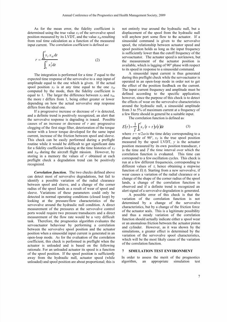
Fidelity coefficient . This check is performed in preflight when the actuator is unloaded or subjectedto little load. The purpose of this check is toevaluate the servovalve dynamic response and tosignal reductions in responding to the changes of theinput current.

While the actuator is in its middle position theentire servoloop is operated in an open-loop modefor a short time, such to limit the actuator travel and

prevent it from hitting its hard stops. While in thisopen-loop mode, an input current is issued to theservovalve as a small positive step, then the currentis brought back to zero with a second step (Fig. 6).

t x xT

eT

M T d1

0∫ −= (1)

SV Block Diagram

[m^2]

AJ

[m^2]

AJ

[m/N*m]

1/KFt

[Pa/m]

GP

[Pa*s/m^3]

GP/GQ

[N/(m/s)]

CJ

[N*m/m]

KSF

[N*m/mA]

GM

[1/s]

GQF/ASV

[1/kg]

1/MJ

XSM

1s

X

XJM

1s

XFM PSR

1s

[mA/m]

GAP

Com[m]

QJ[m^3/s]

Cor [mA]

Err [m]

TM[N*m]

T act[N*m]

XF[m] XS

[m]

Elastic KSF Torque[N*m]

DePC[Pa]

P12th[Pa]

P12[Pa]

DePQ [Pa] FV

F12[N]

Fact[N]

D2XJ[m/s^2]

DXJ[m/s]

XJ[m]

Figure 5: Block diagram of the servoactuator mathematical model used for the prognostic algorithm

Figure 6: Servovalve spool response to a step inputcurrent

Time

Current

x

x T

T




7

As for the mean error, the fidelity coefficient isdetermined using the true value xT of the servovalve spool

position measured by its LVDT, and the value x M resultingfrom real time calculation as a function of the measuredinput current. The correlation coefficient is defined as:

(2)

The integration is performed for a time T equal to theexpected time response of the servovalve to a step input ofamplitude equal to the one which is given. If the actualspool position xT is at any time equal to the one x M computed by the mode, then the fidelity coefficient isequal to 1. The larger the difference between xT and x M ,the more r differs from 1, being either greater or lowerdepending on how the actual servovalve step responsediffers from the ideal one.

If a progressive increase or decrease of r is detected,and a definite trend is positively recognized, an alert thatthe servovalve response is degrading is issued. Possiblecauses of an increase or decrease of r are: progressiveclogging of the first stage filter, deterioration of the torquemotor with a lower torque developed for the same inputcurrent, increase of the friction between spool and sleeve.This check can be easily performed during a preflightroutine while it would be difficult to get significant datafor a fidelity coefficient looking at the time histories of xT and x M during the aircraft flight mission. However, bystoring in a memory the values of r obtained at each

preflight check a degradation trend can be positivelyrecognized.

Correlation function. The two checks defined abovecan detect most of servovalve degradations, but fail toidentify a possible variation of the radial clearance

between spool and sleeve, and a change of the cornerradius of the spool lands as a result of wear of spool andsleeve. Variations of these parameters could only bedetected in normal operating conditions (closed loop) bylooking at the pressure/flow characteristics of theservovalve around the hydraulic null condition. A directmeasurement of the pressures at the servovalve control

ports would require two pressure transducers and a directmeasurement of the flow rate would be a very difficulttask. Therefore, the prognostics algorithm evaluates the

servoactuator behaviour by performing a correlation between the servovalve spool position and the actuator position when a sinusoidal input current is generated in anopen-loop mode. As for the evaluation of the correlationcoefficient, this check is performed in preflight when theactuator is unloaded and is based on the followingrationale. For an unloaded actuator its speed is a functionof the spool position. If the spool position is sufficientlyaway from the hydraulic null, actuator speed (whileunloaded) and spool position are about proportional; this is

not entirely true around the hydraulic null, but adisplacement of the spool from the hydraulic nullwill anyhow port some flow to the actuator. If asinusoidal command is given to the servovalvespool, the relationship between actuator speed andspool position holds as long as the input frequencyis sufficiently lower than the cutoff frequency of the

servoactuator. The actuator speed is not known, butthe measurement of the actuator position isavailable, which is lagging of 90° phase with respectto its speed in response to a sinusoidal command.

A sinusoidal input current is thus generatedduring this preflight check while the servoactuator isoperated in an open-loop mode in order not to getthe effect of the position feedback on the current.The input current frequency and amplitude must bedefined according to the specific application;however, since the purpose of this check is to detectthe effects of wear on the servovalve characteristicsaround the hydraulic null, a sinusoidal amplitudefrom 3 to 5% of maximum current at a frequency of

a few Hertz should in general be a suitable input.The correlation function is defined as:

where τ = π/2ω is the time delay corresponding to a phase angle of 90°, xT is the true spool positionmeasured by the spool LVDT, y is the actuator

position measured by its own position transducer, t is the time and T the time interval over which thecorrelation function is evaluated. This time cancorrespond to a few oscillation cycles. This check isrun at a few different frequencies, corresponding todifferent values of τ , hence obtaining a stepwise

function of E (τ ). Starting from a new servovalve, ifwear causes a variation of the radial clearance or achange of the shape of the corner radius of the spoollands, a change of the correlation function isobserved and if a definite trend is recognized analert signal of a servovalve degradation is generated.

A possible error of this check is that thevariation of the correlation function is notdetermined by a change of the servovalvecharacteristics, but by a change of the friction forceof the actuator seals. This is a legitimate possibilityand thus a steady variation of the correlationfunction should actually indicate either a spool wearor an anomalous friction between the actuator pistonand cylinder. However, as it was shown by thesimulations, a greater effect is determined by thevariation of the servovalve spool characteristics,which will be the most likely cause of the variationof the correlation function.

7 SIMULATION TEST ENVIRONMENT

In order to assess the merit of the prognosticsalgorithm, an appropriate simulation test

∫∫=

T

T

T

M T

t x

t x xr

0

2

0

d

d

( ) ( ) ( ) t t yt xT

E T

T d1

0∫ += τ τ ( ) ( ) ( ) t t yt xT

E T

T d1

0∫ += τ τ ( ) ( ) ( ) t t yt xT

E T

T d1

0∫ += τ τ ( ) ( ) ( ) t t yt xT

E T

T d1

0∫ += τ τ ( ) ( ) ( ) t t yt xT

E T

T d1

0∫ += τ τ ( ) ( ) ( ) t t yt xT

E T

T d1

0∫ += τ τ ( ) ( ) ( ) t t yt xT

E T

T d1

0∫ += τ τ ( ) ( ) ( ) t t yt xT

E T

T d1

0∫ += τ τ (3)




8

environment was defined. Simulations were run in whichan EHSV controlled hydraulic servoactuator was subjectedto time histories of commands and loads representative ofthose that could be encountered during flight, andvariations of the servovalve offset within its normal rangewere simultaneously applied. At the same time,

progressive degradations of the servovalve were

superimposed and the ability of the prognostics algorithmto identify them was verified. The simulation campaignwas performed with reference to a balanced areaservoactuator with the following characteristics:

Stall load: 16000 N at a pressure of 20.7 MPa

Total travel: 400 mm

No-load speed: 300 mm/s

Inertia reflected to actuator linear output: 10 kg

Stiffness of the attachment point (surface): 8x107 N/m

Stiffness of the attachment point (earth): 5x107 N/m

Rated servovalve current: 20 mA

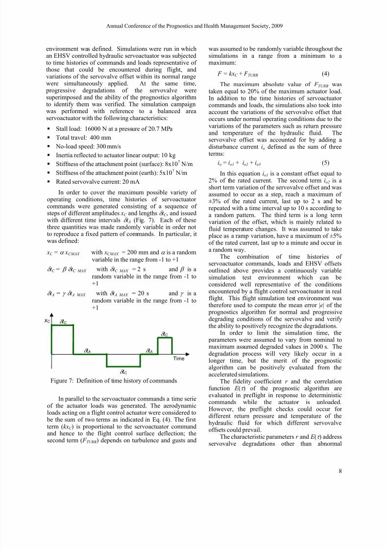
In order to cover the maximum possible variety ofoperating conditions, time histories of servoactuatorcommands were generated consisting of a sequence ofsteps of different amplitudes xC and lengths δ t C , and issuedwith different time intervals δ t A (Fig. 7). Each of thesethree quantities was made randomly variable in order notto reproduce a fixed pattern of commands. In particular, itwas defined:

xC = α xCMAX with xCMAX = 200 mm and α is a random

variable in the range from -1 to +1

δ t C = β δ t C MAX with δ t C MAX = 2 s and β is a

random variable in the range from -1 to+1

δ t A = γ δ t A MAX with δ t A MAX = 20 s and γ is a

random variable in the range from -1 to+1

In parallel to the servoactuator commands a time serieof the actuator loads was generated. The aerodynamicloads acting on a flight control actuator were considered to

be the sum of two terms as indicated in Eq. (4). The firstterm (kxC ) is proportional to the servoactuator commandand hence to the flight control surface deflection; thesecond term ( F TURB) depends on turbulence and gusts and

was assumed to be randomly variable throughout thesimulations in a range from a minimum to amaximum:

F = kxC + F TURB (4)

The maximum absolute value of F TURB wastaken equal to 20% of the maximum actuator load.

In addition to the time histories of servoactuatorcommands and loads, the simulations also took intoaccount the variations of the servovalve offset thatoccurs under normal operating conditions due to thevariations of the parameters such as return pressureand temperature of the hydraulic fluid. Theservovalve offset was accounted for by adding adisturbance current io defined as the sum of threeterms:

io = io1 + io2 + io3 (5)

In this equation io1 is a constant offset equal to2% of the rated current. The second term io2 is ashort term variation of the servovalve offset and was

assumed to occur as a step, reach a maximum of±3% of the rated current, last up to 2 s and berepeated with a time interval up to 10 s according toa random pattern. The third term is a long termvariation of the offset, which is mainly related tofluid temperature changes. It was assumed to take

place as a ramp variation, have a maximum of ±5%of the rated current, last up to a minute and occur ina random way.

The combination of time histories ofservoactuator commands, loads and EHSV offsetsoutlined above provides a continuously variablesimulation test environment which can beconsidered well representative of the conditionsencountered by a flight control servoactuator in realflight. This flight simulation test environment wastherefore used to compute the mean error |e| of the

prognostics algorithm for normal and progressivedegrading conditions of the servovalve and verifythe ability to positively recognize the degradations.

In order to limit the simulation time, the parameters were assumed to vary from nominal tomaximum assumed degraded values in 2000 s. Thedegradation process will very likely occur in alonger time, but the merit of the prognosticalgorithm can be positively evaluated from theaccelerated simulations.

The fidelity coefficient r and the correlationfunction E (τ ) of the prognostic algorithm areevaluated in preflight in response to deterministiccommands while the actuator is unloaded.However, the preflight checks could occur fordifferent return pressure and temperature of thehydraulic fluid for which different servovalveoffsets could prevail.

The characteristic parameters r and E (τ ) addressservovalve degradations other than abnormal

Time

x C

δ t A

δ t C

δ t C

δ t C

δ t A

Figure 7: Definition of time history of commands




9

variations of its offset, and the effects of such degradationscould be partially hidden by the normal offset variationsduring the dedicated preflight checks. Therefore, an initialreading of the spool position and the relevant current must

be performed while the actuator is stationary andunloaded before running the preflight checks. By relatingspool position and current in these conditions the

servovalve offset can be easily derived and acompensating current can be added to the input currentduring the preflight checks thereby ensuring that the initialspool position is the hydraulic null.

However, though the effect of different servovalveoffsets while running the preflight checks can be cancelledout as described above, still the preflight checks performedon a perfectly operational servoactuator can lead to somedifferent values of r and E (τ ) due to variations of the fluid

properties within their normal range as a result of differenttemperatures and amount of free air entrained by thehydraulic fluid. The simulations of the preflight checkswere thus performed assuming that each preflight check

was carried out at a different temperature according to arandom distribution of temperature from -30 °C to +70 °Cand the fluid properties at each temperature wereconsidered. Also, a variable content of free air wasassumed.

8 EFFECTIVENESS OF THE PROGNOSTIC

ALGORITHM

Five different servovalve degradations were considered,that were outlined in paragraph 3, and the ability of the

prognostics algorithm to positively identify them wasassessed. Each degradation was progressively increased ina linear way while continuous variations of the operatingenvironment were simulated as outlined in section 7. Thelinear degradation increase does not represent a limitationfor the evaluation of the effectiveness of the prognosticsalgorithm. In fact, the key point is how well a variation ofa servovalve parameter can be recognized by themathematical model while the other operational

parameters are varying within their normal operatingrange. This can be assessed whichever degradation growth

pattern is used. The effects of servovalve degradations onthe three characteristic parameters of the prognosticsalgorithm are discussed hereunder.

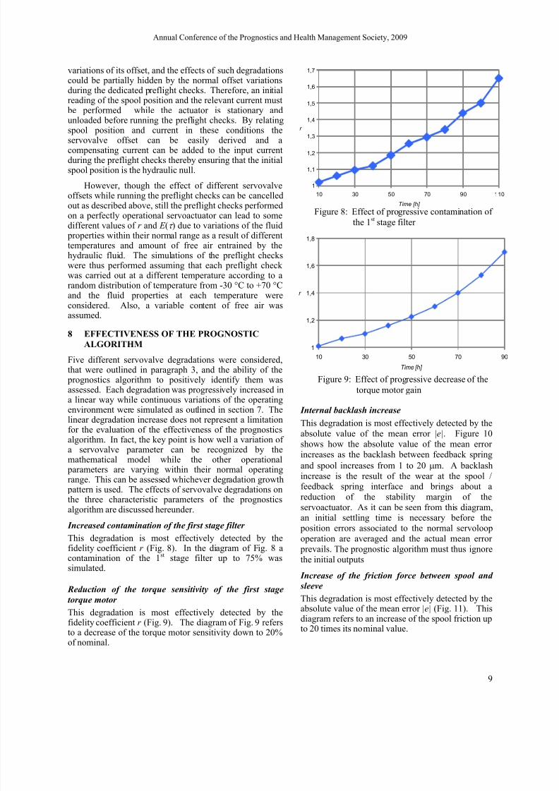
Increased contamination of the first stage filter

This degradation is most effectively detected by thefidelity coefficient r (Fig. 8). In the diagram of Fig. 8 acontamination of the 1st stage filter up to 75% wassimulated.

Reduction of the torque sensitivity of the first stage

torque motor

This degradation is most effectively detected by thefidelity coefficient r (Fig. 9). The diagram of Fig. 9 refersto a decrease of the torque motor sensitivity down to 20%of nominal.

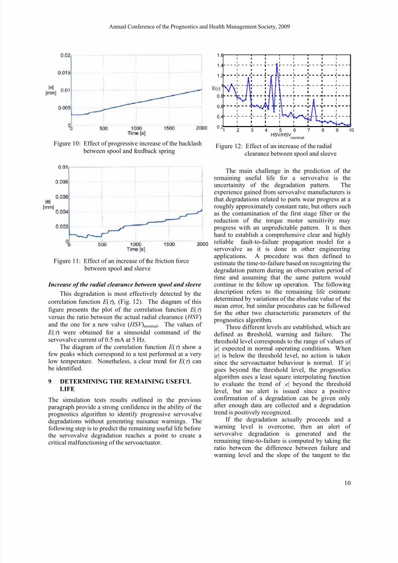
Internal backlash increase

This degradation is most effectively detected by the

absolute value of the mean error |e|. Figure 10

shows how the absolute value of the mean error

increases as the backlash between feedback spring

and spool increases from 1 to 20 μm. A backlash

increase is the result of the wear at the spool /feedback spring interface and brings about a

reduction of the stability margin of the

servoactuator. As it can be seen from this diagram,an initial settling time is necessary before the

position errors associated to the normal servoloop

operation are averaged and the actual mean error

prevails. The prognostic algorithm must thus ignore

the initial outputs

Increase of the friction force between spool and

sleeve

This degradation is most effectively detected by theabsolute value of the mean error |e| (Fig. 11). Thisdiagram refers to an increase of the spool friction upto 20 times its nominal value.

Figure 8: Effect of progressive contamination of

the 1st stage filter

1

1,1

1,2

1,3

1,4

1,5

1,6

1,7

10 30 50 70 90 110

Time [h]

r

Figure 9: Effect of progressive decrease of the

torque motor gain

1

1,2

1,4

1,6

1,8

10 30 50 70 90

Time [h]

r




10

Increase of the radial clearance between spool and sleeve

This degradation is most effectively detected by thecorrelation function E (τ ), (Fig. 12). The diagram of this

figure presents the plot of the correlation function E (τ )

versus the ratio between the actual radial clearance ( HSV )

and the one for a new valve ( HSV )nominal. The values of

E (τ ) were obtained for a sinusoidal command of theservovalve current of 0.5 mA at 5 Hz.

The diagram of the correlation function E (τ ) show afew peaks which correspond to a test performed at a verylow temperature. Nonetheless, a clear trend for E (τ ) can

be identified.

9 DETERMINING THE REMAINING USEFUL

LIFE

The simulation tests results outlined in the previous paragraph provide a strong confidence in the ability of the prognostics algorithm to identify progressive servovalvedegradations without generating nuisance warnings. Thefollowing step is to predict the remaining useful life beforethe servovalve degradation reaches a point to create acritical malfunctioning of the servoactuator.

The main challenge in the prediction of theremaining useful life for a servovalve is theuncertainity of the degradation pattern. Theexperience gained from servovalve manufacturers is

that degradations related to parts wear progress at aroughly approximately constant rate, but others suchas the contamination of the first stage filter or thereduction of the torque motor sensitivity may

progress with an unpredictable pattern. It is thenhard to establish a comprehensive clear and highlyreliable fault-to-failure propagation model for aservovalve as it is done in other engineeringapplications. A procedure was then defined toestimate the time-to-failure based on recognizing thedegradation pattern during an observation period oftime and assuming that the same pattern wouldcontinue in the follow up operation. The followingdescription refers to the remaining life estimatedetermined by variations of the absolute value of themean error, but similar procedures can be followedfor the other two characteristic parameters of the

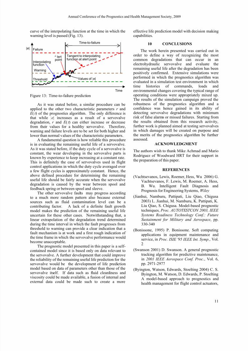
prognostics algorithm.Three different levels are established, which are

defined as threshold, warning and failure. Thethreshold level corresponds to the range of values of|e| expected in normal operating conditions. When|e| is below the threshold level, no action is takensince the servoactuator behaviour is normal. If |e|goes beyond the threshold level, the prognosticsalgorithm uses a least square interpolating functionto evaluate the trend of |e| beyond the thresholdlevel, but no alert is issued since a positiveconfirmation of a degradation can be given onlyafter enough data are collected and a degradationtrend is positively recognized.

If the degradation actually proceeds and awarning level is overcome, then an alert ofservovalve degradation is generated and theremaining time-to-failure is computed by taking theratio between the difference between failure andwarning level and the slope of the tangent to the

Figure 10: Effect of progressive increase of the backlash

between spool and feedback spring

Figure 11: Effect of an increase of the friction force

between spool and sleeve

Figure 12: Effect of an increase of the radial

clearance between spool and sleeve

1 2 3 4 5 6 7 8 9 100.2

0.4

0.6

0.8

1

1.2

1.4

1.6

HSV/HSVnominal

E(τ)




11

curve of the interpolating function at the time in which thewarning level is passed (Fig. 13).

As it was stated before, a similar procedure can beapplied to the other two characteristic parameters r and

E (τ ) of the prognostics algorithm. The only difference isthat while |e| increases as a result of a servovalve

degradation, r and E (τ ) can either increase or decreasefrom their values for a healthy servovalve. Therefore,warning and failure levels are to be set for both higher andlower than normal values of the characteristic parameters.

A fundamental question is how reliable this procedureis in evaluating the remaining useful life of a servovalve.As it was stated before, if the duty cycle of a servovalve isconstant, the wear developing in the servovalve parts isknown by experience to keep increasing at a constant rate.This is definitely the case of servovalves used in flightcontrol applications in which the duty cycle averaged overa few flight cycles is approximately constant. Hence, theabove defined procedure for determining the remaininguseful life should be fairly accurate when the servovalve

degradation is caused by the wear between spool andfeedback spring or between spool and sleeve.

The other servovalve faults may progress accordingto a much more random pattern also because externalsources such as fluid contamination level can be acontributing factor. A lack of a definite fault growthmodel makes the prediction of the remaining useful lifeuncertain for these other cases. Notwithstanding that, alinear extrapolation of the degradation trend determinedduring the time interval in which the fault progresses fromthreshold to warning can provide a clear indication that afault mechanism is at work and a first rough indication ofthe time frame in which the servovalve performance would

become unacceptable.

The prognostic model presented in this paper is a self-contained model since it is based only on data relevant tothe servovalve. A further development that could improvethe reliability of the remaining useful life prediction for theservovalve would be the development of life predictionmodel based on data of parameters other than those of theservovalve itself. If data such as fluid cleanliness andviscosity could be made available, a fusion of internal andexternal data could be made such to create a more

effective life prediction model with decision makingcapabilities.

10 CONCLUSIONS

The work herein presented was carried out inorder to define a way of recognizing the most

common degradations that can occur in anelectrohydraulic servovalve and evaluate theremaining useful life after the degradation has been

positively confirmed. Extensive simulations were performed in which the prognostics algorithm wasevaluated in a simulation test environment in whichtime histories of commands, loads andenvironmental changes covering the typical range ofoperating conditions were appropriately mixed up.The results of the simulation campaign proved therobustness of the prognostics algorithm and aconfidence was hence gained in its ability ofdetecting servovalve degradations with minimumrisk of false alarms or missed failures. Starting from

the results obtained from this research activity,further work is planned aimed at testing servovalvesin which damages will be created on purpose andthe merits of the prognostics algorithm be furtherassessed.

ACKNOWLEDGMENT

The authors wish to thank Mike Achmad and Mario

Rodriguez of Woodward HRT for their support inthe preparation of this paper.

REFERENCES

(Vachtsevanos, Lewis, Roemer, Hess, Wu 2006) G.Vachtsevanos, F. Lewis, M. Roemer, A. Hess,

B. Wu. Intelligent Fault Diagnosis andPrognosis for Engineering Systems, Wiley

(Jianhui, Namburu, Pattipati, Liu Qiao, Chigusa

2003) L. Jianhui, M. Namburu, K. Pattipati, K.Liu Qiao, S. Chigusa. Model-based prognostic

techniques, Proc. AUTOTESTCON 2003, IEEE

Systems Readiness Technology Conf.: FutureSustainment for Military and Aerospace, pp.

330-340

(Bonissone, 1995) P. Bonissone. Soft computing

applications in equipment maintenance andservice, in Proc. ISIE '95 IEEE Int. Symp., Vol.

2(Swanson 2001) D. Swanson. A general prognostic

tracking algorithm for predictive maintenance,

in 2001 IEEE Aerospace Conf. Proc., Vol. 6, pp. 2971-2977

(Byington, Watson, Edwards, Stoelting 2004) C. S.

Byington, M. Watson, D. Edwards, P. Stoelting

A model-based approach to prognostics andhealth management for flight control actuators,

Time

Threshold

Warning

Failure

Time-to-failure

|e|

Values of |e|

Interpolatingfunction

lertpoint

Tangent to interpolatingfunction at alert point

Figure 13: Time-to-failure prediction




12

2004 IEEE Aerospace Conf. Proc., Vol. 6, pp. 3551-

3562

(Jaw, Wang 2006) L. C. Jaw, W. Wang. Mathematical

Formulation of Model-Based Methods for

Diagnostics and Prognostics, in Proc. GT2006 ASMETurbo Expo 2006: Power for Land, Sea and Air ,

Barcelona, Spain(Watson, Byington 2006) M. Watson, C.S. Byington.

Improving the maintenance process and enabling

prognostics for control actuators using CAHM

software, 2006 IEEE Aerospace Conf. Proc.

(Jacazio, Borello 1988) G. Jacazio, L. Borello.

Mathematical Models of Electrohydraulic

Servovalves for Fly-by-Wire Flight ControlSystems, in Mathematical Computational

Modelling, Vol. 11, ppp. 563-569, PergamonPress

Documents

11-Borello Electrohydraulic Servovalves