NBER WORKING PAPER SERIES

THE LIQUIDITY TRAP AND ThE PIGOU EFFECT:A DYNAMIC ANALYSIS WITH RATIONAL EXPECTATIONS

Bennett T. McCallum

Working Paper No. 891k

NATIONAL BUREAU OF ECONOMIC RESEARCH1050 Massachusetts Avenue

Cambridge M! 02138

May 1982

I am indebted to Larry Summers, James Tobin, and seminar par-ticipants at Yale University for helpful comments on an earlierversion and to the National Science Foundation for financial sup-port (SES T9—15353). The research reported here is part of theNBER's research program in Economic Fluctuations. Any opinionsexpressed are those of the author and not those of the NationalBureau of Economic Research.

NBER Working Paper #894May 1982

The Liquidity Trap and the Pigou Effect: A DynamicAnalysis with Rational Expectations

Abstract

A Keynesian idea of considerable historical importance is that, in the

presence of a liquidity trap, a competitive economy may lack——despite price

flexibility——automatic market mechanisms that tend to eliminate excess supplies

of labor. The standard classical counterargument, which relies upon the Pigou

effect, has typically been conducted in a comparative—static framework. But,

as James Tobin has recently emphasized, the more relevant issue concerns the

dynamic response (in "real time") of an economy that has been shocked away from

full employment. The present paper develops a dynamic analysis, in a rather

standard model, under the assumption that expectations are formed rationally.

The analysis permits examination of Tobin's suggestion that, because of expecta—

tional effects, such an economy could be unstable. Also considered is Martin

J. Bailey's conjecture that, in the absence of a stock Pigou effect, Keynesian

problems could be eliminated by expectational influences on disposable income.

Bennett T. McCallumGraduate School of IndustrialAdministration

Carnegie—Mellon UniversityPittsburgh, PA 15213

(412) 578—2347

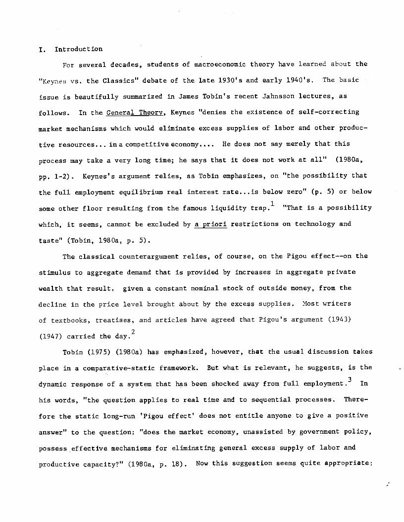
I. Introduction

For several decades, students of macroeconomic theory have learned about the

"Keynes vs. the Classics" debate of the late 1930's and early 1940's. The basic

issue is beautifully summarized in James Tobin's recent Jahnsson lectures, as

follows. In the General Theory, Keynes "denies the existence of self—correcting

market mechanisms which would eliminate excess supplies of labor and other produc-

tive resources... in a competitive economy.... He does not say merely that this

process may take a very long time; he says that it does not work at all" (l980a,

pp. 1-2). Keynes's argument relies, as Tobin emphasizes, on "the possibility that

the full employment equilibrium real interest rate.. . is below zero" (p. 5) or below

some other floor resulting from the famous liquidity trap.1 "That is a possibility

which, it seems, cannot be excluded by a priori restrictions on technology and

taste" (Tobin, 1980a, p. 5).

The classical counterargument relies, of course, on the Pigou effect——on the

stimulus to aggregate demand that is provided by increases in aggregate private

wealth that result, given a constant nominal stock of outside money, from the

decline in the price level brought about by the excess supplies. Most writers

of textbooks, treatises, and articles have agreed that Pigou's argument (1943)

(1947) carried the day.2

Tobin (1975) (1980a) has emphasized, however, that the usual discussion takes

place in a comparative—static framework. But what is relevant, he suggests, is the

dynamic response of a system that has been shocked away from full employment.3 In

his words, "the question applies to real time and to sequential processes. There-

fore the static long—run 'Pigou effect' does not entitle anyone to give a positive

answer" to the question: "does the market economy, unassisted by government policy,

possess effective mechanisms for eliminating general excess supply of labor and

productive capacity?" (1980a, p. 18). Now this suggestion seems quite appropriate:

—2—

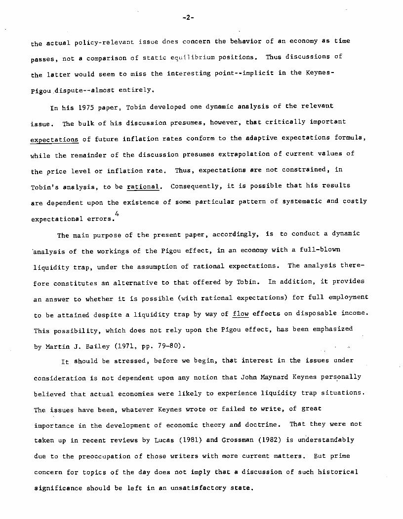
the actual policy-relevant issue does concern the behavior of an economy as time

passes, not a comparison of static equilibrium positions. Thus discussions of

the latter would seem to miss the interesting point--implicit in the Keynes—

pigou dispute--almost entirely.

In his 1975 paper, Tobirt developed one dynamic analysis of the relevant

issue. The bulk of his discussion presumes, however, that critically important

expectations of future inflation rates conform to the adaptive expectations formula,

while the remainder of the discussion presumes extrapolation of current values of

the price level or inflation rate. Thus, expectations are not constrained, in

Tobin's analysis, to be rational, Consequently, it is possible that his results

are dependent upon the existence of some particular pattern of systematic and costly

4expectational errors.

The main purpose of the present paper, accordingly, is to conduct a dynamic

'analysis of the workings of the Pigou effect, in an economy with a full—blown

liquidity trap, under the assumption of rational expectations. The analysis there-

fore constitutes an alternative to that offered by Tobin. In addition, it provides

an answer to whether it is possible (with rational expectations) for full employment

to be attained despite a liquidity trap by way of flow effects on disposable income.

This possibility, which does not rely upon the Pigou effect, has been emphasized

by Martin J. Bailey (1971, pp. 79—80).

it should be stressed, before we begin, that interest in the issues under

consideration is not dependent upon any notion that John Maynard Keynes personally

believed that actual economies were likely to experience liquidity trap situations.

The issues have been, whatever Keynes wrote or failed to write, of great

importance in the development of economic theory and doctrine. That they were not

taken up in recent reviews by Lucas (1981) and Grossman (1982) is understandably

due to the preoccupation of those writers with more current matters. But prime

concern for topics of the day does not imply that a discussion of such historical

significance should be left in an unsatisfactory state.

—3.-

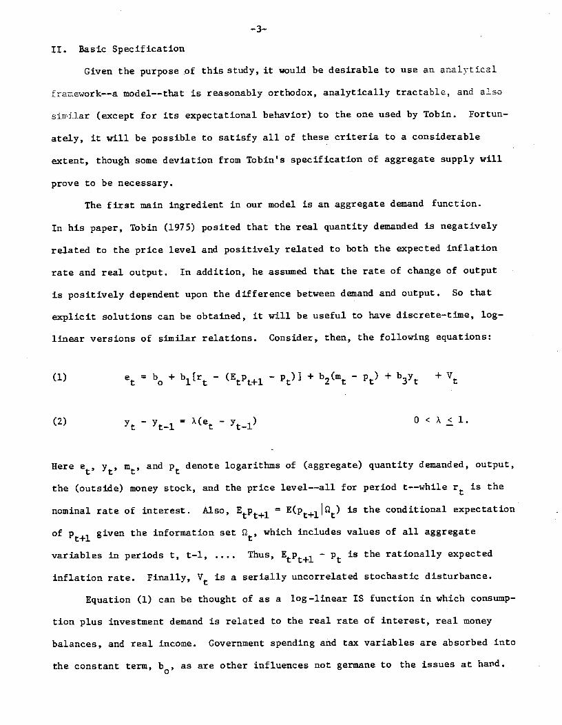
II. Basic Specification

Given the purpose of this study, it would be desirable to use an analytical

framework——a model——that is reasonably orthodox, analytically tractable, and also

similar (except for its expectational behavior) to the one used by Tobin. Fortun-

ately, it will be possible to satisfy all of these criteria to a considerable

extent, though some deviation from Tobin's specification of aggregate supply will

prove to be necessary.

The first main ingredient in our model is an aggregate demand function.

In his paper, Tobin (1975) posited that the real quantity demanded is negatively

related to the price level and positively related to both the expected inflation

rate and real output. In addition, he assumed that the rate of change of output

is positively dependent upon the difference between demand and output. So that

explicit solutions can be obtained, it will be useful to have discrete—time, log—

linear versions of similar relations. Consider, then, the following equations:

(1) e = b + bi[r — (Ep÷i — + b2(m — + b3y + Vt

(2) — = X(e — 0 < A - 1.

Here e, y, n', and Pt denote logarithms of (aggregate) quantity demanded, output,

the (outside) money stock, and the price level——all for period t——while r is the

nominal rate of interest. Also, Etpt+i = E(p÷1Ic2) is the conditional expectation

E given the information set S, which includes values of all aggregate

variables in periods t, t—l Thus, Etpt+1 — Pt is the rationally expected

inflation rate. Finally, V is a serially uncorrelated stochastic disturbance.

Equation (1) can be thought of as a log—linear IS function in which consump-

tion plus investment demand is related to the real rate of interest, real money

balances, and real income. Government spending and tax variables are absorbed into

the constant term, b, as are other influences not germane to the issues at hard.

—4—

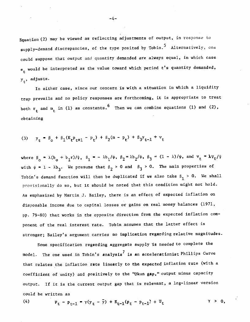
Equation (2) may be viewed as reflecting adjustments of output, in response. to

supply—demand discrepancies, of the type posited by Tobin.5 Alternatively, on

could suppose that output and quantity demanded are always equal, in which case

e would be interpreted as the value toward which period t's quantity demanded,

adjusts.

In either case, since our concern is with a situation in which a liquidity

trap prevails and no policy responses are forthcoming, it is appropriate to treat

both rt and m in (1) as constants.6 Then we can combine equations (1) and (2),

obtaining

= o + i(Etp+i — + (m — p) + 3t—l ÷

where f3. = X(b0 + b1r)/$,= — Xb1/,

2=Ab2/,= (1 — X)/, and v

with = 1 —Ab3.

We presume that 2 > 0 and > 0. The main properties of

Tobin's demand function will then be duplicated if we also take > 0. We shall

provisionally do so, but it should be noted that this condition might not hold.

As emphasized by Martin J. Bailey, there is an effect of expected inflation on

disposable income due to capital losses or gains on real money balances (1971,

pp. 79—80) that works in the opposite direction from the expected inflation com-

ponent of the real interest rate. Tobin assumes that the latter effect is

stronger; Bailey's argument carries no implication regarding relative magnitudes.

Some specification regarding aggregate supply is needed to complete the

model. The one used in Tobin's analysis7 is an accelerationist Phillips Curve

that relates the inflation rate linearly to the expected inflation rate (with a

coefficient of unity) and positively to the "Okun gap," output minus capacity

output. If it is the current output gap that is relevant, a log—linear version

could be written as

— nt—i = i(y — ) + Et...i(pt — + U r > 0,

—5—

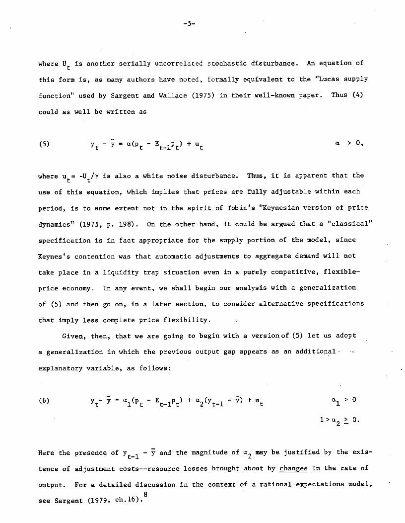
where U is another serially uncorrelated stochastic disturbance. An equation of

this form is, as many authors have noted, formally equivalent to the "Lucas supply

function" used by Sargent and Wallace (1975) in their well—known paper. Thus (4)

could as well be written as

— = a(p — EiPt) + u >

where u= -u" is also a white noise disturbance. Thus, it is apparent that the

use of this equation, which implies that prices are fully adjustable within each

period, is to some extent not in the spirit of Tobin's "Keynesian version of price

dynamics" (1975, p. 198). On the other hand, it could be argued that a "classical"

specification is in fact appropriate for the supply portion of the model, since

Keynes's contention was that automatic adjustments to aggregate demand will not

take place in a liquidity trap situation even in a purely competitive, flexible—

price economy. In any event, we shall begin our analysis with a generalization

of (5) and then go on, in a later section, to consider alternative specifications

that imply less complete price flexibility.

Given, then, that we are going to begin with a version of (5) let us adopt

a generalization in which the previous output gap appears as an additional

explanatory variable, as follows:

(6). yt—= a1(p

— Eip) + c2(yi — Y) + u a1 > 0

l>a2>O.

Here the presence of — y and the magnitude of a2 may be justified by the exis-

tence of adjustment costs——resource losses brought about by changes in the rate of

output. For a detailed discussion in the context of a rational expectations model,

see Sargent (1979, ch.16).8

—6—

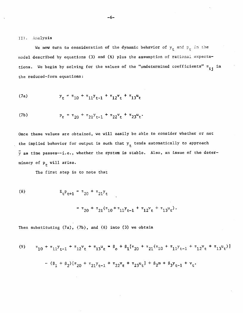
Jil. Analysis

We now turn to consideration of the dynamic behavior of y and p in the

model described by equations (3) and (6) plus the assumption of rational expecta-

tions. We begin by solving for the values of the "undetermined coefficients" in

the reduced—form equations:

(7a) = + + irv +

(7b) Pt = 2O + 2lt—l + 22t +

Once these values are obtained, we will easily be able to consider whether or not

the implied behavior for output is such that y tends automatically to approach

y as time passes——i.e., whether the system is stable. Also, an issue of the deter—

minacy of Pt will arise.

The first step is to note that

(8) Etpt+l r20 +

=2O + 2l iOlit—i ÷ ir12v + 1r13u).

Then substituting (7a), (7b), and (8) into (3) we obtain

(9) lO + llt—l + l2t + l3t = 8o+ + 2llO + 1ltl + 12v + 13u)}

+ 2)N20 + 1y1 + 22v + 23u] ÷ 2m + 3t1 + v.

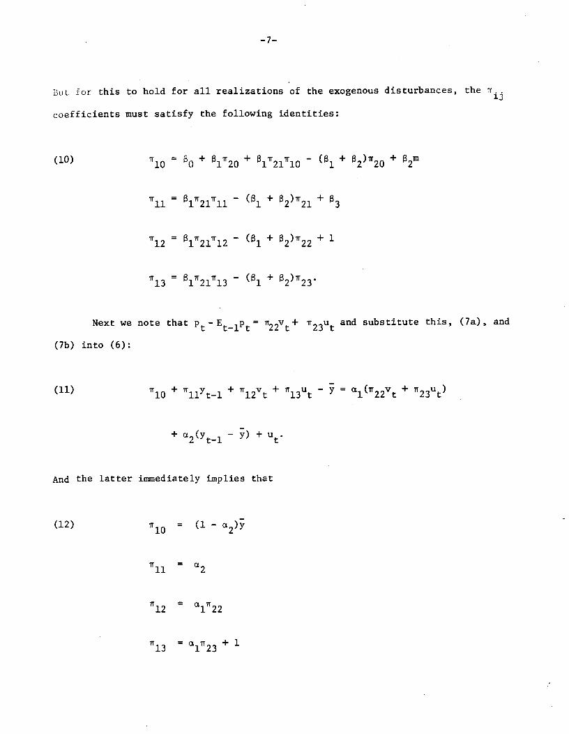
—7—

But. for this to hold for all realizations •of the exogenous disturbances, the

coefficients must satisfy the following identities:

(10) Tf10 o + l2O + 8l2llO — l + 22O + 2m

'ill = l2lll — 1 + 22l +

l2 = ]Y2fTl2- l + 82)r22 + 1

l3 = l2ll3 — l + 223

Next we note that pt_Et_1pt 22\+ r23u. and substitute this, (7a), and

(7b) into (6):

(11) l0 + llt-1 + l2t + 13u — = ai(22v + 23u)

+ 2t—l — + Ut.

And the latter immediately implies that

(12) = (1 —

11 =

12 = 122

l3 = + 1

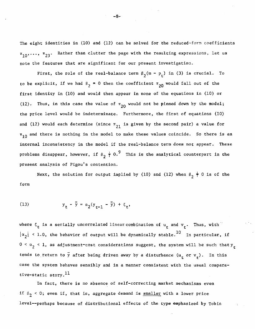
—8—

The eight identities in (10) and (12) can be solved for the reduced—form coefficients

lO'"' 23 Rather than clutter the page with the resulting expressions, let us

note the features that are significant for our present investigation.

First, the role of the real—balance term 132(m — in (3) is crucial. To

to be explicit, if we had 2 = 0 then the coefficient 2O would fall out of the

first identity in (10) and would then appear in none of the equations in (10) or

(12). Thus, in this case the value of 2O would not be pinned down by the model;

the price level would be indeterminate. Furthermore, the first of equations (10)

and (12) would each determine (since 2l is given by the second pair) a value for

lO and there is nothing in the model to make these values coincide. So there is an

internal inconsistency in the model if the real—balance term does not appear. These

problems disappear, however, if 2 + This is the analytical counterpart in the

present analysis of Pigou's contention.

Next, the solution for output implied by (10) and (12) when 2 + 0 is of the

form

(13) = a2y — ) + ,

where is a serially uncorrelated linear combination of u and v. Thus, with

1a21 < 1.0, the behavior of output will be dynamically stable.1° In particular, if

0 < 2 < 1, as adjustment—cost considerations suggest, the system will be such thaty

tends to,return to y after being driven away by a disturbance (u or vt). In this

case the system behaves sensibly and in a manner consistent with the usual compara-

tive—static story.11

In fact, there is no absence of self—correcting market mechanisms even

2 < 0; even if, that is, aggregate demand is smaller with a lower price

level——perhaps because of distributional effects of the type emphasized by Tobin

— 9-.

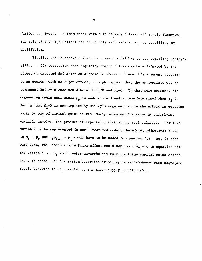
(1980a, pp. 9—11). In this model with a relatively "classical" supply function,

the role of the Pigou effect has to do only with existence, not stability, of

equilibrium.

Finally, let us consider what the present model has to say regarding Bailey's

(1971, p. 80) suggestion that liquidity trap problems may be eliminated by the

effect of expected deflation on disposable income. Since this argument pertains

to an economy with no Pigou effect, it might appear that the appropriate way to

represent Bailey's case would be with ]<0 and 2=0 If that were correct, his

suggestion would fail since Pt IS undetermined and overdetermined when I2=0.

But in fact 2=0 is not implied by Bailey's argument: since the effect in question

works by way of capital gains on real money balances, the relevant underlying

variable involves the product of expected inflation and real balances. For this

variable to be represented in our linearized model, therefore, additional terms

in m - and Etpt÷i - would have to be added to equation (1). But if that

were done, the absence of a Pigou effect would not imply 2 = 0 in equation (3):

the variable m - p would enter nevertheless to reflect the capital gains effect.

Thus, it seems that the system described by Bailey is well-behaved when aggregate

supply behavior is represented by the Lucas supply function (6).

—10—

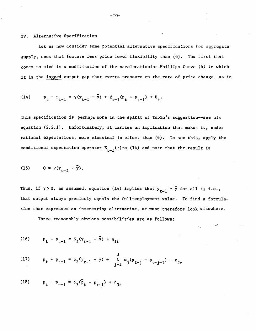
IV. Alternative Specification

Let us now consider some potential alternative specifications for aggregate

supply, ones that feature less price level flexibility than (6). The first that

comes to mind is a modification of the accelerationist Phillips Curve (4) in which

it is the lagged output gap that exerts pressure on the rate of price change, as in

(14) Pt 1_l = t—l — + Ei(p — + U.

This specification is perhaps more in the spirit of Tobin's suggestion——see his

equation (2.2.1). Unfortunately, it carries an implication that makes it, under

rational expectations, more classical in effect than (6). To see this, apply the

conditional expectation operator Ei()to (14) and note that the result is

(15) 0 = t—l —

Thus, if y>O, as assumed, equation (14) implies that = y for all t; i.e.,

that output always precisely equals the full—employment value. To find a formula-

tion that expresses an interesting alternative, we must therefore look elsewhere.

Three reasonably obvious possibilities are as follows:

(16) Pt — -i = lt—l — + 11t

(17) Pt — Pti =62t—1

- +j1

— +

(18) Pt — t—l 63t — '—) +

-P11—

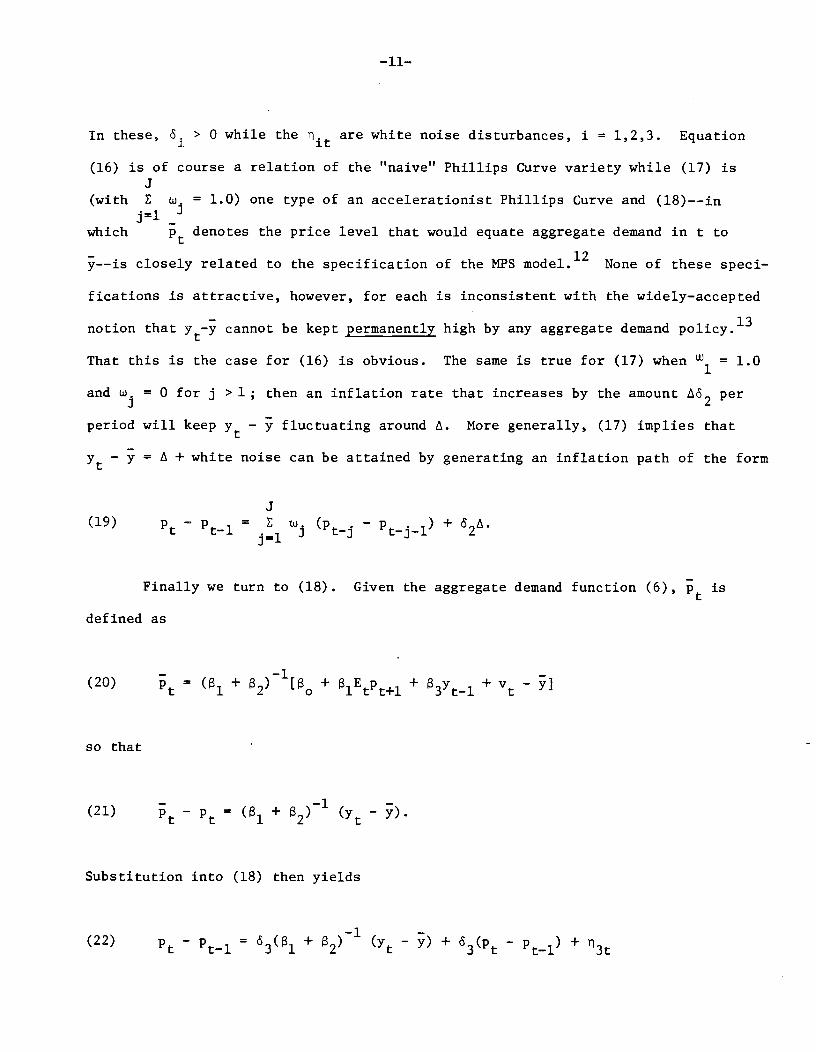
In these, 5. > 0 while the are white noise disturbances, i = 1,2,3. Equation

(16) is of course a relation of the 11naive Phillips Curve variety while (17) isJ

(with E w. = 1.0) one type of an accelerationist Phillips Curve and (18)—-jn

j=l•

which Pt denotes the price level that would equate aggregate demand in t to

——is closely related to the specification of the MPS model.12 None of these speci-

fications is attractive, however, for each is inconsistent with the widely—accepted

notion that cannot be kept permanently high by any aggregate demand policy.13

That this is the case for (16) is obvious. The same is true for (17) when = 1.0

and w. 0 for j > 1 ; then an inflation rate that increases by the amount s2 per

period will keep y — y fluctuating around . More generally, (17) implies that

— = + white noise can be attained by generating an inflation path of the form

(19) Pt — _ij=l

i t-j - t-J—l +

Finally we turn to (18). Given the aggregate demand function (6), p is

defined as

(20) = l + + iEP +i + 83_1 + v

so that

(21) -Pt

= + -

Substitution into (18) then yields

(22) Pt - t—l = 31 + 82)- y) + 3t - +

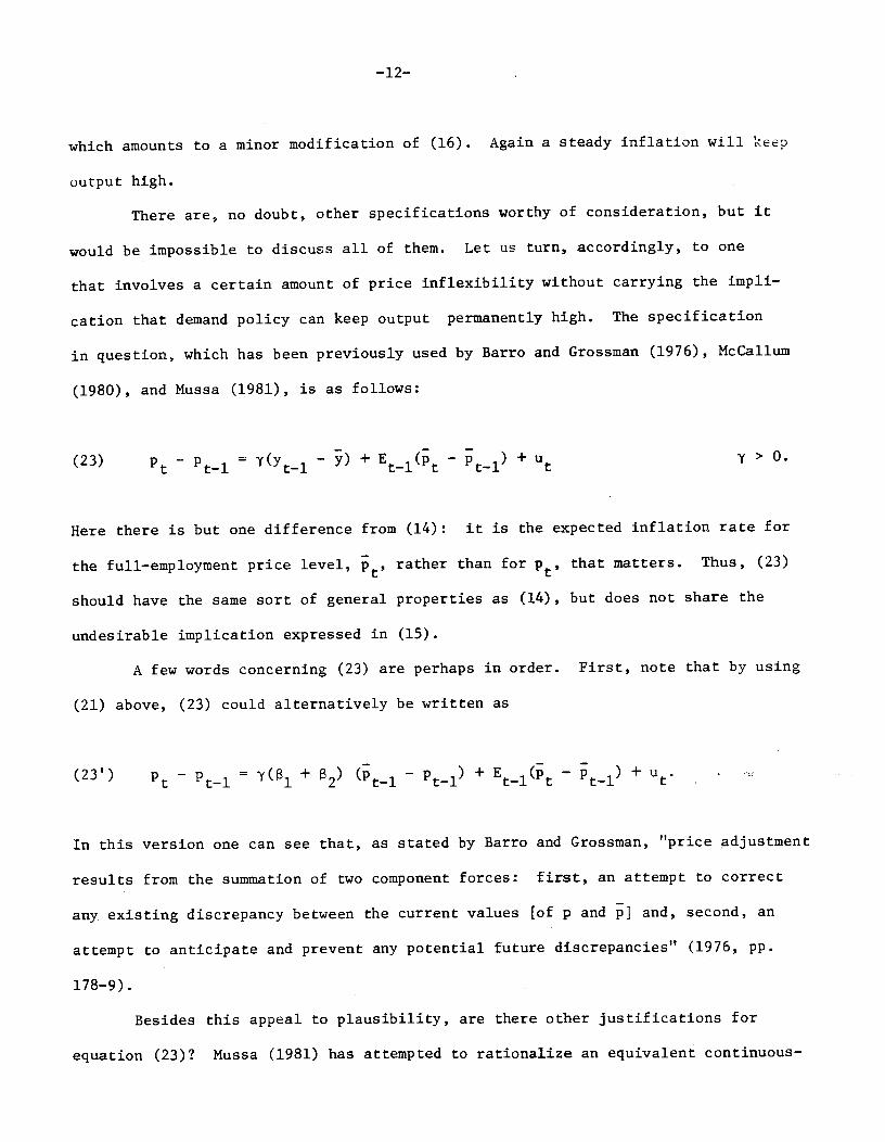
—12--

which amounts to a minor modification of (16). Again a steady inflation will keep

output high.

There are, no doubt, other specifications worthy of consideration, but it

would be impossible to discuss all of them. Let us turn, accordingly, to one

that involves a certain amount of price inflexibility without carrying the impli-

cation that demand policy can keep output permanently high. The specification

in question, which has been previously used by Barro and Grossman (1976), McCallum

(1980), and Mussa (1981), is as follows:

(23) Pt t—l = 't—l — y) + Ei(p t—1 + u y > 0.

Here there is but one difference from (14): it is the expected inflation rate for

the full—employment price level, p, rather than for p, that matters. Thus, (23)

should have the same sort of general properties as (14), but does not share the

undesirable implication expressed in (15).

A few words concerning (23) are perhaps in order. First, note that by using

(21) above, (23) could alternatively be written as

(23') Pt — Pti = "l + t—1 — + Ei(p — t—1 + u.

In this version one can see that, as stated by Barro and Grossman, "price djustment

results from the summation of two component forces: first, an attempt to correct

any, existing discrepancy between the current values [of p and and, second, an

attempt to anticipate and prevent any potential future discrepancies" (1976, pp.

178—9).

Besides this appeal to plausibility, are there other justifications for

equation (23)? Mussa (1981) has attempted to rationalize an equivalent continuous—

—13—

time specification in terms of profit maximizing behavior by firms that incur

significant lump—sum costs from changing prices, while McCallum (1980) has pro-

posed an alternative rationale that appeals to optimizing behavior on the part

of worker—firm agents that experience employment adjustment costs and must set

prices in advance. These arguments are open to certain objections,14 but never-

theless seem to place (23) on a firmer basis than most sticky—price specifications.

Accordingly, let us now consider the dynamic behavior of output in a model con-

sisting of equations (3) and (23), with rational expectations.

The first step is to rearrange (23) as follows:

(24) Pt — = "— — + 1_ — + u.

Next, from equation (20) and its counterpart with and y in place of

and y, we note that

(25) Pt — Etlt = l + z)[i(Etp+i — Etip+i) + v — —

Using (25) and (21) in (24) then yields, after rearrangement,15

(26) yt — = — + 1(Ep÷i — E 1+1 + v — ( +

where 1 — y(1 +

As in the analysis in Section III, solutions for y and Pt will be of the

form (7) while Etpt+i is again representable by (8). Reference to (8) shows, more-

over, that E = 7T20 + 21lo + rry so we easily obtain

—14—

(27) EtPt÷l= 21(12v i3u).

Substitution of (27) and (7a) into (26) then yields the identities

(28)= (1 —

1111=

it12 TT21T12 + 1

= lt2ltl3 - l +

The identities implied by the demand portion of the model remain the same as

before, so the relevant conclusions can be drawn from equations (7), (10), and

(28).

In several ways, these conclusions are as in Section III. Again, if

= 0 —— if the Pigou and capital gains effects are absent —— there will be no

solution for r20 and two for r10,so again the price level will be undetermined

and output overdetermined by the model.

Again, furthermore, output relative to capacity obeys a first—order auto-

regressive process, in this case

(29) = — +

with white noise. But now dynamic stability depends upon the magnitude of

= 1 — y(1 2' rather than a2. Let us first consider the standard case, in

which and 2' as well as y, are positive. Given the form of , these sign

conditions alone do not indicate whether stability will prevail. But the

—15—

Parameters are such that coherent thought about their quantitative magnitudes

is possible. Let us suppose that the model's time periods correspond to quarter—

years. Then the magnitude of y and will be very small, in comparison to 1.0,

so will almost certainly be a positive fractioJ6——which, of course, implies

that y is stable and tends to approach y as time passes. Since the model is

not recursive, Pt will therefore also be stable.

If either or is negative, however, it is possible that their sum will

be negative, in which case 4 will exceed 1.0 and the system will be unstable.

In the present context it is worth noting that both Tobin and Bailey have suggested

that 2 might not be positive —— because of distributional effects (Tobin) or the

dominance of capital gains over Pigou effects (Bailey). Thus, these suggestions

give some impetus to the idea that instability might prevail. But given the

widely—held belief that distributional, wealth, and capital—gains effects are

all quantitatively minor, it seems likely that the sign of + 82 will be deter-

mined by 81 and that will be positive because of the depressing effect of the

real interest rate on aggregate demand. All in all, then, the analysis of this

section provides little support for the idea that instability would prevail if

aggregate supply were not perfectly classical.

—16—

V. Conclusion

Our results can be briefly summarized as follows. In a macroeconomic

model with a liquidity trap, a Lucas—type "classical" aggregate supply function,

and rational expectations, the system is well—behaved and dynamically stable if

either the Pigou effect or the capital—gains effect of expected inflation on dis-

posable income is present. If both are absent, the model fails to determine the

price level and is internally inconsistent. If the Lucas—type supply function

is replaced with a "disequilibrium" specification that relates price changes to the

previous level of excess demand and to the expected change in the full—employment

price level, the system is again determinate if the Pigou or capital—gains effect

is operative. In this case dynamic stability cannot be guaranteed but instability

seems rather unlikely.

Re ferences

Bailey, Martin j National Income and the Price Level, 2nd. ed. (New York:

McGraw-Hill, 1971).

Barro, Robert J., and Herschel I. Grossman. Money, Employment, and Inflation.

(Cambridge: Cambridge University Press, 1976).

Blaug, Mark. Economic Theory in Retrospect, 2nd. ed. (Homewood, IL.,: Irwin,

1968).

Gordon, Robert J. Macroeconomics, 2nd. ed. (Boston: Little, Brown and Co., 1981).

Grossman, Herschel I. Review of Asset Accumulation and Economic Activity,

by James Tobin. Journal of Monetary Economics 9 (1982), forthcoming.

Keynes, John Maynard, The General Theory of Employment, Interest, and Money.

(London: Macmillan, 1936).

Leijonhufvud, Axel. On Keynesian Economics and the Economics of Keynes.

(New York: Oxford University Press, 1968).

Lucas, Robert E., Jr. Review of A Model of Macroeconomic Activity, Vol. 1,

by Ray C. Fair. Journal of Economic Literature 8 (Sept. 1975), 889—90.

___________________ "Tobin and Monetarism: A Review Article," Journal of

Economic Literature 19 (June 1981), 558-567.

McCallum, Bennett T. "Rational Expectations and Macroeconomic Stabilization

Policy: An Overview," Journal of Money, Credit, and Banking 12

(November 1980, Part 2), 716-746.

___________________ 'Monetarism, Rational Expectations, Oligopolistic Pricing,

and the MPS Econometric Model," Journal of Political Economy 87

(February 1979), 57-73.

__________________ "On Non-Uniqueness in Rational Expectations Models: An

Attempt at Perspective." NBER Working Paper No. 684, June 1981.

Mussa, Michael. "Sticky Individual Prices and the Dynamics of the General

Price Level." In Carnegie-Rochester Conference Series Vol. 15, edited

by K. Brunner and A. H. Meltzer. (Amsterdam: North Holland, 1981).

Okun, Arthur N. "Efficient Deflationary Policies," American Economic Review

Papers and Proceedings 68 (March 1978), 348-352.

Patinkin, Don. Mortey Interest, and Prices, 2nd. ed. (New York: Harper and

Row, 1965).

_____________ "Keynesian Economics Rehabilitated: A Rejoinder to Professor

Hicks," Economic Journal 69 (September 1959), 582-587.

Pigou, A. C. "The Classical Stationary State," Economic Journal 53 (December 1943),

343 -35 1.

___________ "Economic Progress in a Stable Economics 14

(August 1947), 180-188.

Sargent, Thomas J. Macroeconomic Theory (New York: Academic Press, 1979).

Sargent, Thomas J., and Neil Wallace. "Rational' Expectations, the Optimal

Monetary Instrument, and the Optimal Money Supply Rule," Journal of Political

Economy 83 (April 1975), 241-254.

TobirL, James. "Keynesian Models of Recession and Depression," American Economic

Review Papers and Proceedings 65 (May 1975), 195-202.

____________ Asset Accumulation and Economic Activity. (Chicago: University

of Chicago Press, 1980). (a)

____________ "Are New Classical Models Plausible Enough to Guide Policy?"

Journal of Money, Credit, and Banking 12 (November 1980, Part 2),

788-799. (b)

Footnotes

1. There is a second strand to the discussion in the General Theory that stresses

the importance of unions, relative wage concerns by individuals, and generally

the fact that money wages are set in a non—auction marketplace. But, as Tobin

points out, this strand "serves better to emphasize the difficulty and slowness

of melting frozen wage levels or wage—increase patterns than to establish that

they never melt at all" (p.3). It does not buttress Keynes's truly radical claim,

that there is no automatic tendency for full employment to be restored even .if

wages do adjust.

2. See, for example, Blaug (1968, p.648) Gordon (1981, pp. 160—3), Sargent (1979,

pp. 63—65), and Patinkin (1959) (1965). These authors mention, but do not

emphasize, the dynamic considerations with which the present paper is concerned.

3. The discussion here, and in what follows, is not meant to imply that the

"full employment" rate of employment or output is constant, smoothly growing, or

clearly discernable to econometricians. It might be better to use the term "mar-

ket—clearing," as in Barro and Grossman (1976). This paper will, however, retain

the more traditional terminology.

4. For discussions of the desirability of using rational expectations in macro-

economic analysis, see Lucas (1975) and McCallum (1980).

5. It would be possible to interpret Tobin's continuous—time equations as suggesting

—1—l

= A(ei — rather than (1). It seems inappropriate, however, to

make output in a period independent of that period's demand influences.

6. This treatment is consistent with Tobin's (1975).

7. Reference is to Tobin's WPK model, not his M model, as the former is the one

that he presents as representing aspects of Keynes's theory and in which he detects

the possibility of dynamic instability of output.

8. Tobiri (1980b) is on record as objecting to the inclusion of lagged output

terms in equations like (6). He is of course correct in claiming that the inclu—

sion has no relation (one way or the other) to rational expectations. Whether

it has "very thin intrinsic justification" (p. 791) is debatable. In what follows,

the exclusion of — y would not alter the main theoretical conclusions but

would impart a characteristic to the model——absence of unemployment persistence——

that seems counterfactual.

9. This last conclusion is similar to those reached by Bailey (1971, pp. 51—54)

and Sargent (1979, p. 63) in static contexts.

10. The same is true for p. Since the model is not fully recursive, the auto-

regressive parts in ARNA representations are the same for both endogenous variables

and stability depends only upon the autoregressive components.

11. This statement ignores the possibility of "bubble" or "bootstrap" paths, involv-

ing solution equations more general in form than (7), that can occur in dynamic

models with rational or irrational expectations. The issues raised by this

possibility of multiple solutions are only weakly related to those of concern in

the present paper. For an extensive discussion, see McCallum (1981).

12. On this point, see McCallum (1979).

13. The following discussion presumes that demand management (monetary and fiscal

policy) can be used to generate arbitrary price level paths.

14. The assumptions in McCallum (1980), for example, imply that it is prohibitively

costly to change prices within a period, but relatively costless to do so across

periods. In addition, it presumes that period length is determined exogenously.

15. Unlike the analogous equation (25) in McCallum (1980), expression (26) does

not support the controversial "policy ineffectiveness" proposition: monetary policy

rules may affect the magnitude of 2l in (27) below and thereby the variance of

— y. This difference results from differing assumptions regarding information

tvailable to agents in forming expectations about that are relevant to

perceptions of the real interest rate. For some discussion of the relevant

issue, see McCallum (1980, pp. 736—8).

16. Even if the time periods are years, the values of y and will be small

relative to 1.0. A value for y of 0.1, for example, reflects the well—known

rule—of—thumb that "the cost of a 1 point reduction in the basic inflation rate

is 10 percent of a year's GNP" (Okun, 1978, p. 348). While rational expectations

analysis leads one to doubt the validity of Okun's estimate of the unemployment

costs of a policy change, it does not suggest that the implied "estimate" of y is

seriously wrong.