100GbE in Datacenter Interconnects: When, Where?

1

Where?Bikash KoleyNetwork Architecture, Google

Sep 2009

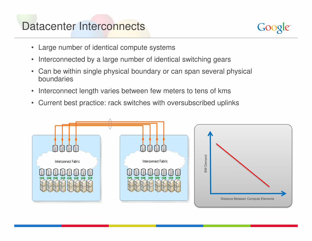
Datacenter Interconnects

• Large number of identical compute systems

• Interconnected by a large number of identical switching gears

• Can be within single physical boundary or can span several physical boundaries

• Interconnect length varies between few meters to tens of kms

• Current best practice: rack switches with oversubscribed uplinks

Distance Between Compute Elements

BW

Dem

and

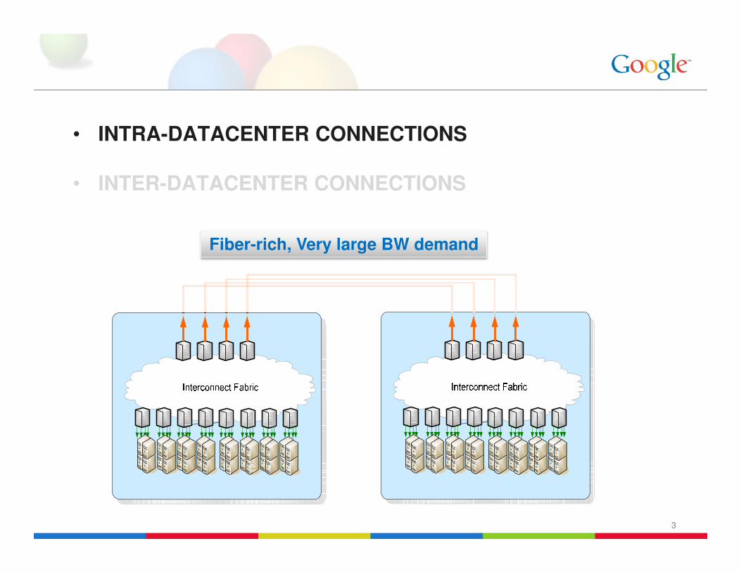
• INTRA-DATACENTER CONNECTIONS

• INTER-DATACENTER CONNECTIONS

Fiber-rich, Very large BW demand

3

Datacenter Interconnect Fabrics

• High performance computing/ super-computing architectures have often used various complex multi-stage fabric architectures such as Clos Fabric, Fat Tree or Torus [1, 2, 3, 4, 5]

• For this theoretical study, we picked the Fat Tree architecture described in [2, 3], and analyzed the impact of choice of interconnect speed and technology on overall interconnect cost

• As described in [2,3], Fat-tree fabrics are built with identical N-port switching elements

• Such a switch fabric architecture delivers a constant bisectional bandwidth (CBB)

N/2

Spines

A 2-stage Fat TreeA 3-stage Fat Tree

4

1. C. Clos, A study of non-blocking switching networks, Bell System Technical Journal, Vol. 32, 1953, pp. 406-424.2. Charles E. Leiserson: “Fat-Trees: Universal Networks for Hardware-Efficient Supercomputing.”, IEEE Transactionson Computers, Vol 34, October 1985, pp 892-9013. S. R. Ohring, M. Ibel, S. K. Das, M. J. Kumar, “On Generalized Fat-tree,” IEEE IPPS 1995.4 RUFT: Simplifying the Fat-Tree Topology, Gomez, C.; Gilabert, F.; Gomez, M.E.; Lopez, P.; Duato, J.; Parallel and Distributed Systems, 2008. ICPADS '08. 14th IEEE International

Conference on, 8-10 Dec. 2008 Page(s):153 – 1605. [Beowulf] torus versus (fat) tree topologies: http://www.beowulf.org/archive/2004-November/011114.html

Interconnect at What Port Speed?

• A switching node has a fixed switching capacity (i.e. CMOS gate-count) within the same space and power envelope

• Per node switching capacity can be presented at different port-speed:

– i.e. a 400Gbps node can be 40X10Gbps or 10X40Gbps or 4X100Gbps

3-stage Fat-tree Fabric Capacity

100

1,000

10,000

100,000

1,000,000

Maxim

al F

ab

ric C

ap

acit

y (

Gb

ps)

5

4X100Gbps

• Lower per-port speed allows building a much larger size maximal constant bisectional bandwidth fabric

• There are of course trade-offs with the number of fiber-connections needed to build the interconnect

• Higher port-speed may allow better utilization of the fabric capacity

1

10

0 100 200 300 400 500 600 700 800

Maxim

al F

ab

ric C

ap

acit

y (

Gb

ps)

Per Node Switching Capacity (Gbps)

Port Speed = 10 Gbps

Port Speed = 40Gbps

Port Speed = 100Gbps

Fabric Size vs Port Speed

Constant switching BW/node of 1Tbps and constant fabric cross-section BW of 10Tbps Assumed

No of Fabric Stages Needed for a 10T Fabric

0

2

4

6

8

10

12

14

No o

f F

abric S

tages N

eeded

Switching_BW/node=1Tbps

5

spines

6

0

0 100 200 300 400 500

Port Speed (Gbps)

No of Fabric Nodes Needed for a 10T Fabric

0

1000

2000

3000

4000

5000

6000

7000

0 50 100 150 200 250 300 350 400

Port Speed (Gbps)

No o

f N

odes N

eeded

Switching_BW/node=1Tbps

• Higher per port bandwidth reduces the number of available ports in a node with constant switching bandwidth•In order to support same cross-sectional BW

�more stages are needed in the fabric �More fabric nodes are needed

Power vs Port Speed

Per Port Power Consumption

40

60

80

100

120

140

Per-

po

rt P

ow

er

Co

nsu

mp

tio

n (

Watt

s)

Constant power/Gbps

4x power for 10x speed

20x power for 10x speed

Total Interconnect Power Consumption

100000

150000

200000

250000

300000

To

tal P

ow

er

Co

nsu

mp

tio

n (

Watt

s)

Constant power/Gbps

4x power for 10x speed

20x power for 10x speed

BLEEDING EDGE

POWER PARITY

BLEEDING EDGE

POWER PARITY

7

• Three power consumption curves for interface optical modules:

– Bleeding Edge: 20x power for 10x speed; e.g. if 10G is 1W/port, 100G is 20W/port

– Power Parity: Power parity on per Gbps basis; e.g. if 10G is 1W/port, 100G is 10W/port

– Mature: 4x power for 10x speed; e.g. if 10G is 1W/port, 100G is 4W/port

• Lower port speed provides lower power consumption

• For power consumption parity, power per optical module needs to follow the “mature” curve

0

20

0 50 100 150 200 250 300 350 400 450

Port Speed (Gbps)

Per-

po

rt P

ow

er

Co

nsu

mp

tio

n (

Watt

s)

0

50000

0 50 100 150 200 250 300 350 400

Port Speed (Gbps)

MATURE MATURE

PARITY

Cost vs Port Speed

Per Port Optics Cost

$20,000

$30,000

$40,000

$50,000

$60,000

$70,000

Per-

po

rt O

pti

cs C

ost

Constant cost/Gbps

4x cost for 10x speed

20x cost for 10x speed

Total Fabric Cost

$60,000,000

$80,000,000

$100,000,000

$120,000,000

$140,000,000

$160,000,000

To

tal F

ab

ric

Co

st

Constant cost/Gbps

4x cost for 10x speed

20x cost for 10x speedBLEEDING EDGE

COST PARITY

BLEEDING EDGE

COST PARITY

8

$0

$10,000

$20,000

0 50 100 150 200 250 300 350 400 450

Port Speed (Gbps)

$0

$20,000,000

$40,000,000

0 50 100 150 200 250 300 350 400

Port Speed (Gbps)

MATUREMATURE

COST PARITY

• Three cost curves for optical interface modules:– Bleeding Edge: 20x cost for 10x speed

– Cost Parity: Cost parity on per Gbps basis

– Mature: 4x cost for 10x speed;

• Fiber cost is assumed to be constant per port (10% of 10G port cost)

• For fabric cost parity, cost of optical modules need to increase by < 4x for 10x increase in interface speed

• INTRA-DATACENTER CONNECTIONS

• INTER-DATACENTER CONNECTIONS

Limited Fiber Availability, 2km+ reach

9

Beyond 100G: What data rate?

• 400Gbps? 1Tbps? Something “in-between”? How about all of the above?

•Current optical PMD specs are designed for absolute worst-case penalties

•Significant capacity is untapped within the statistical variation of various penalties

10

“Wasted

Link

Margin/

Capacity

Where is the Untapped Capacity?

-60

-50

-40

-30

-20

-10

0

Receiver Performance

Sen

sit

ivit

y (

dB

m)

Optical Channel Capacity

M. Nakazawa: ECOC 2008

11

-80

-70

1.00E-02 1.00E-01 1.00E+00 1.00E+01 1.00E+02 1.00E+03

Quantum limit of

Sensitivity

Bit Rate (Gbps)

• Unused Link Margin ≡ Untapped SNR ≡ Untapped Capacity

• In ideal world, 3dB of link margin will allow link capacity to be doubled

• Need the ability to use additional capacity (speed up the link) when available (temporal or statistical) and scale-back to the base-line capacity (40G/100G?) when not

M. Nakazawa: ECOC 2008paper Tu.1.E.1

Rate Adaptive 100G+ Ethernet?

• There are existing standards within the IEEE802.3 family:

• IEEE 802.3ah 10PASS-TS: based on MCM-VDSL standard

• IEEE 802.3ah 2BASE-TL: based on SHDSL standard

• Needed when channels are close to physics-limit : We are getting there with 100Gbps+ Ethernet

• Shorter links ≡ Higher capacity (matches perfectly with datacenter bandwidth demand distribution, see slide # 3)

600

12

0

100

200

300

400

500

0 2 4 6 8 10 12 14 16 18

Bit

Ra

te (

Gb

ps)

SNR (dB)

mQAM

OOK

• How to get there?

• High-order modulation

• Multi-carrier-Modulation/OFDM

• Ultra-dense WDM

• Combination of all the above

Is There a Business Case?

0

0.05

0.1

0.15

0.2

0.25

0 10 20 30 40 50

Dis

trib

uti

on

Link Distance (km)

Example Link Distance Distribution

0

100

200

300

400

500

600

0 10 20 30 40 50

Po

ssib

le B

it R

tae

(G

bp

s)

Link Distance (km)

Example Adaptive Bit Rate Implementations

scheme-1

scheme-2

non-adaptive

13

Link Distance (km)Link Distance (km)

0

50

100

150

200

250

300

350

400

0 100 200 300 400 500 600

Tota

l Ca

pa

cit

y o

n 1

00

0 lin

ks

(Tb

ps)

Max Adaptive Bit Rate with 100Gbps base rate (Gbps)

Aggregate Capacity for 1000 Links • An example link-length distribution between datacenters is shown

• Can be supported by a 40km capable PMD

• Various rate-adaptive 100GbE+ options are considered

• Base rate is 100Gbps

• Max adaptive bit-rate varies from 100G to 500G

• Aggregate capacity for 1000 such links is computed

Q&A