FRE

EC

OP

Y10

Shortest PathsM

G

F

N

PK

S

QO

R

L

0

5

11

13

15

1718

1920

Distance to M

17

C

H

VJ

W

E

The problem of the shortest, quickest or cheapest path is ubiquitous. You solve itdaily. When you are in a location s and want to move to a location t, you ask for thequickest path from s to t. The fire department may want to compute the quickest routesfrom a fire station s to all locations in town – the single-source problem. Sometimeswe may even want a complete distance table from everywhere toeverywhere – theall-pairs problem. In a road atlas, you will usually find an all-pairs distance tablefor the most important cities.

Here is a route-planning algorithm that requires a city map and a lot of dexteritybut no computer. Lay thin threads along the roads on the city map. Make a knotwherever roads meet, and at your starting position. Now liftthe starting knot untilthe entire net dangles below it. If you have successfully avoided any tangles and thethreads and your knots are thin enough so that only tight threads hinder a knot frommoving down, the tight threads define the shortest paths. Theintroductory figure ofthis chapter shows the campus map of the University of Karlsruhe1 and illustratesthe route-planning algorithm for the source node M.

Route planning in road networks is one of the many applications of shortest-path computations. When an appropriate graph model is defined, many problemsturn out to profit from shortest-path computations. For example, Ahuja et al. [8]mentioned such diverse applications as planning flows in networks, urban housing,inventory planning, DNA sequencing, the knapsack problem (see also Chap. 12),production planning, telephone operator scheduling, vehicle fleet planning, approx-imating piecewise linear functions, and allocating inspection effort on a productionline.

The most general formulation of the shortest-path problem looks at a directedgraphG = (V,E) and a cost functionc that maps edges to arbitrary real-number

1 (c) Universität Karlsruhe (TH), Institut für Photogrammetrie und Fernerkundung.

FRE

EC

OP

Y192 10 Shortest Paths

costs. It turns out that the most general problem is fairly expensive to solve. So weare also interested in various restrictions that allow simpler and more efficient al-gorithms: nonnegative edge costs, integer edge costs, and acyclic graphs. Note thatwe have already solved the very special case of unit edge costs in Sect. 9.1 – thebreadth-first search (BFS) tree rooted at nodes is a concise representation of allshortest paths froms. We begin in Sect. 10.1 with some basic concepts that lead toa generic approach to shortest-path algorithms. A systematic approach will help usto keep track of the zoo of shortest-path algorithms. As our first example of a re-stricted but fast and simple algorithm, we look at acyclic graphs in Sect. 10.2. InSect. 10.3, we come to the most widely used algorithm for shortest paths: Dijkstra’salgorithm for general graphs with nonnegative edge costs. The efficiency of Dijk-stra’s algorithm relies heavily on efficient priority queues. In an introductory courseor at first reading, Dijkstra’s algorithm might be a good place to stop. But there aremany more interesting things about shortest paths in the remainder of the chapter.We begin with an average-case analysis of Dijkstra’s algorithm in Sect. 10.4 whichindicates that priority queue operations might dominate the execution time less thanone might think. In Sect. 10.5, we discussmonotone priority queues for integer keysthat take additional advantage of the properties of Dijkstra’s algorithm. Combiningthis with average-case analysis leads even to a linear expected execution time. Sec-tion 10.6 deals with arbitrary edge costs, and Sect. 10.7 treats the all-pairs problem.We show that the all-pairs problem for general edge costs reduces to one generalsingle-source problem plusn single-source problems with nonnegative edge costs.This reduction introduces the generally useful concept of node potentials. We closewith a discussion of shortest path queries in Sect. 10.8.

10.1 From Basic Concepts to a Generic Algorithm

We extend the cost function to paths in the natural way. The cost of a path is thesum of the costs of its constituent edges, i.e., ifp = 〈e1,e2, . . . ,ek〉, thenc(p) =

∑1≤i≤k c(ei). The empty path has cost zero.For a pairs andv of nodes, we are interested in a shortest path froms to v. We

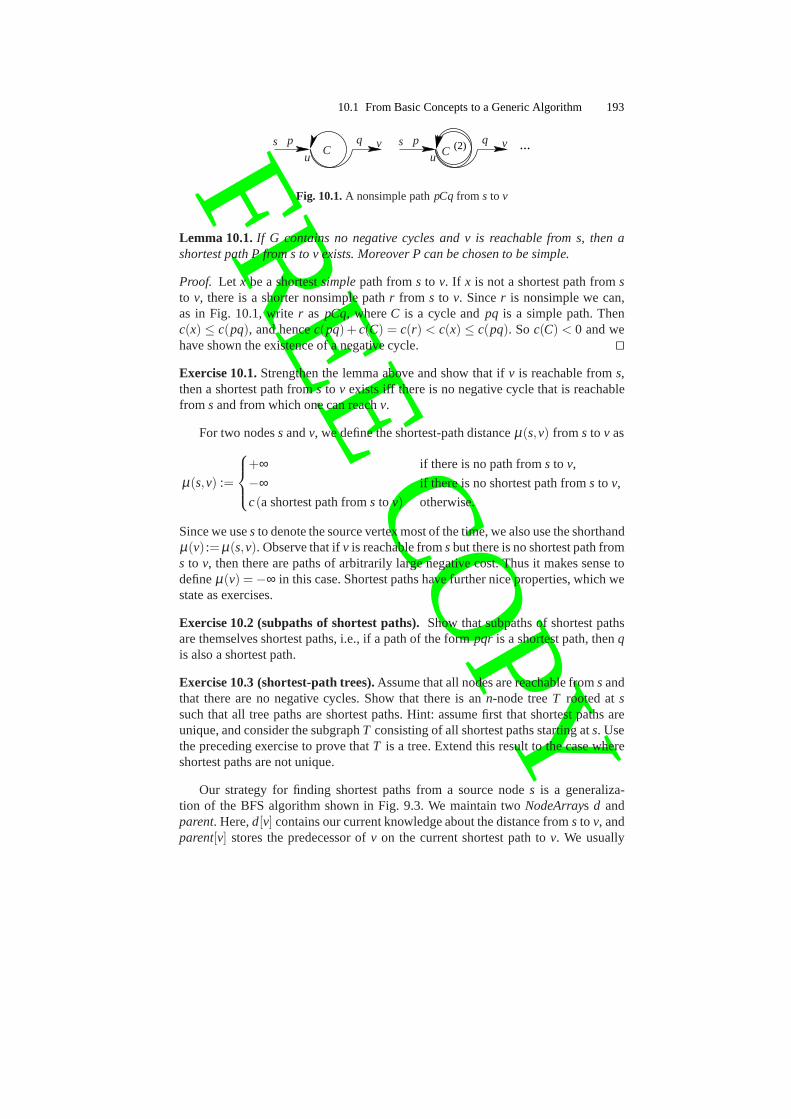
avoid the use of the definite article “the” here, since there may be more than oneshortest path. Does a shortest path always exist? Observe that the number of pathsfrom s to v may be infinite. For example, ifr = pCq is a path froms to v containing acycleC, then we may go around the cycle an arbitrary number of times and still havea path froms to v; see Fig. 10.1. More precisely,p is a path leading froms to u, C isa path leading fromu to u, andq is a path fromu to v. Consider the pathr(i) = pCiqwhich first usesp to go froms to u, then goes around the cyclei times, and finallyfollows q from u to v. The cost ofr(i) is c(p)+ i ·c(C)+c(q). If C is anegative cycle,i.e.,c(C) < 0, thenc(r(i+1)) < c(r(i)). In this situation, there is no shortest path froms to v. Assume otherwise: say,P is a shortest path froms to v. Thenc(r(i)) < c(P)for i large enough2, and soP is not a shortest path froms to v. We shall show nextthat shortest paths exist if there are no negative cycles.

2 i > (c(p)+c(q)−c(P))/|c(C)| will do.

FRE

EC

OP

Y10.1 From Basic Concepts to a Generic Algorithm 193

...(2)p ps sq qCC

v vuu

Fig. 10.1.A nonsimple pathpCqfrom s to v

Lemma 10.1.If G contains no negative cycles and v is reachable from s, then ashortest path P from s to v exists. Moreover P can be chosen to be simple.

Proof. Let x be a shortestsimplepath froms to v. If x is not a shortest path fromsto v, there is a shorter nonsimple pathr from s to v. Sincer is nonsimple we can,as in Fig. 10.1, writer as pCq, whereC is a cycle andpq is a simple path. Thenc(x) ≤ c(pq), and hencec(pq)+ c(C) = c(r) < c(x) ≤ c(pq). Soc(C) < 0 and wehave shown the existence of a negative cycle. ⊓⊔

Exercise 10.1.Strengthen the lemma above and show that ifv is reachable froms,then a shortest path froms to v exists iff there is no negative cycle that is reachablefrom sand from which one can reachv.

For two nodessandv, we define the shortest-path distanceµ(s,v) from s to v as

µ(s,v) :=

+∞ if there is no path froms to v,

−∞ if there is no shortest path froms to v,

c(a shortest path froms to v) otherwise.

Since we uses to denote the source vertex most of the time, we also use the shorthandµ(v) :=µ(s,v). Observe that ifv is reachable fromsbut there is no shortest path froms to v, then there are paths of arbitrarily large negative cost. Thus it makes sense todefineµ(v) = −∞ in this case. Shortest paths have further nice properties, which westate as exercises.

Exercise 10.2 (subpaths of shortest paths).Show that subpaths of shortest pathsare themselves shortest paths, i.e., if a path of the formpqr is a shortest path, thenqis also a shortest path.

Exercise 10.3 (shortest-path trees).Assume that all nodes are reachable fromsandthat there are no negative cycles. Show that there is ann-node treeT rooted atssuch that all tree paths are shortest paths. Hint: assume first that shortest paths areunique, and consider the subgraphT consisting of all shortest paths starting ats. Usethe preceding exercise to prove thatT is a tree. Extend this result to the case whereshortest paths are not unique.

Our strategy for finding shortest paths from a source nodes is a generaliza-tion of the BFS algorithm shown in Fig. 9.3. We maintain twoNodeArrays d andparent. Here,d[v] contains our current knowledge about the distance froms to v, andparent[v] stores the predecessor ofv on the current shortest path tov. We usually

FRE

EC

OP

Y194 10 Shortest Paths

42

0

0

0

0

52

2−1

−1−1−2

−2

−2−3

−3

+∞

−∞−∞ −∞

−∞

a b d f g

hijk s

Fig. 10.2.A graph with shortest-path distancesµ(v). Edge costs are shown as edge labels, andthe distances are shown inside the nodes. The thick edges indicate shortest paths

refer tod[v] as thetentative distanceof v. Initially, d[s] = 0 andparent[s] = s. Allother nodes have infinite distance and no parent.

The natural way to improve distance values is to propagate distance informationacross edges. If there is a path froms to u of costd[u], ande= (u,v) is an edge outof u, then there is a path froms to v of costd[u]+ c(e). If this cost is smaller thanthe best previously known distanced[v], we updated andparentaccordingly. Thisprocess is callededge relaxation:

Procedurerelax(e= (u,v) : Edge)if d[u]+c(e) < d[v] then d[v] :=d[u]+c(e); parent[v] :=u

Lemma 10.2.After any sequence of edge relaxations, if d[v] < ∞, then there is apath of length d[v] from s to v.

Proof. We use induction on the number of edge relaxations. The claimis certainlytrue before the first relaxation. The empty path is a path of length zero froms tos, and all other nodes have infinite distance. Consider next a relaxation of an edgee= (u,v). By the induction hypothesis, there is a pathp of lengthd[u] from s to uand a path of lengthd[v] from s to v. If d[u]+c(e) ≥ d[v], there is nothing to show.Otherwise,pe is a path of lengthd[u]+c(e) from s to v. ⊓⊔

The common strategy of the algorithms in this chapter is to relax edges until ei-ther all shortest paths have been found or a negative cycle isdiscovered. For example,the (reversed) thick edges in Fig. 10.2 give us theparentinformation obtained after asufficient number of edge relaxations: nodesf , g, i, andh are reachable fromsusingthese edges and have reached their respectiveµ(·) values 2,−3,−1, and−3. Nodesb, j, andd form a negative-cost cycle so that their shortest-path costis −∞. Nodeais attached to this cycle, and thusµ(a) = −∞.

What is a good sequence of edge relaxations? Letp = 〈e1, . . . ,ek〉 be a path froms to v. If we relax the edges in the ordere1 to ek, we haved[v] ≤ c(p) after thesequence of relaxations. Ifp is a shortest path froms to v, thend[v] cannot dropbelow c(p), by the preceding lemma, and henced[v] = c(p) after the sequence ofrelaxations.

Lemma 10.3 (correctness criterion). After performing a sequence R of edge re-laxations, we have d[v] = µ(v) if, for some shortest path p= 〈e1,e2, . . . ,ek〉 from

FRE

EC

OP

Y10.2 Directed Acyclic Graphs 195

s to v, p is a subsequence of R, i.e., there are indices t1 < t2 < · · · < tk such thatR[t1] = e1,R[t2] = e2, . . . ,R[tk] = ek. Moreover, the parent information defines a pathof lengthµ(v) from s to v.

Proof. The following is a schematic view ofRandp: the first row indicates the time.At time t1, the edgee1 is relaxed, at timet2, the edgee2 is relaxed, and so on:

1,2, . . . , t1, . . . , t2, . . . . . . ,tk, . . .R:= 〈 . . . ,e1, . . . , e2, . . . . . . ,ek, . . .〉p:= 〈e1, e2, . . . ,ek〉

We haveµ(v) = ∑1≤ j≤k c(ej). For i ∈ 1..k, let vi be the target node ofei , and wedefinet0 = 0 andv0 = s. Thend[vi ]≤∑1≤ j≤i c(ej) after timeti , as a simple inductionshows. This is clear fori = 0, sinced[s] is initialized to zero andd-values are onlydecreased. After the relaxation ofei = R[ti ] for i > 0, we haved[vi ]≤d[vi−1]+c(ei)≤∑1≤ j≤i c(ej). Thus, after timetk, we haved[v] ≤ µ(v). Sinced[v] cannot go belowµ(v), by Lemma 10.2, we haved[v] = µ(v) after timetk and hence after performingall relaxations inR.

Let us prove next that theparentinformation traces out shortest paths. We shalldo so under the additional assumption that shortest paths are unique, and leave thegeneral case to the reader. After the relaxations inR, we haved[vi ] = µ(vi) for 1≤i ≤ k. Whend[vi ] was set toµ(vi) by an operationrelax(u,vi), the existence of a pathof lengthµ(vi) from s to vi was established. Since, by assumption, the shortest pathfrom s to vi is unique, we must haveu = vi−1, and henceparent[vi ] = vi−1. ⊓⊔Exercise 10.4.Redo the second paragraph in the proof above, but without theas-sumption that shortest paths are unique.

Exercise 10.5.Let S be the edges ofG in some arbitrary order and letS(n−1) ben−1 copies ofS. Show thatµ(v) = d[v] for all nodesv with µ(v) 6= −∞ after therelaxationsS(n−1) have been performed.

In the following sections, we shall exhibit more efficient sequences of relaxationsfor acyclic graphs and for graphs with nonnegative edge weights. We come back togeneral graphs in Sect. 10.6.

10.2 Directed Acyclic Graphs

In a directed acyclic graph (DAG), there are no directed cycles and hence no negativecycles. Moreover, we have learned in Sect. 9.2.1 that the nodes of a DAG can betopologically sorted into a sequence〈v1,v2, . . . ,vn〉 such that(vi ,v j) ∈ E impliesi < j. A topological order can be computed in linear time O(m+n) using eitherdepth-first search or breadth-first search. The nodes on any path in a DAG increasein topological order. Thus, by Lemma 10.3, we can compute correct shortest-pathdistances if we first relax the edges out ofv1, then the edges out ofv2, etc.; seeFig. 10.3 for an example. In this way, each edge is relaxed only once. Since everyedge relaxation takes constant time, we obtain a total execution time of O(m+n).

FRE

EC

OP

Y196 10 Shortest Paths

3

9

s1

45

2 7

68

Fig. 10.3.Order of edge relaxations for the computation of the shortest paths from nodes in aDAG. The topological order of the nodes is given by theirx-coordinates

Theorem 10.4.Shortest paths in acyclic graphs can be computed in timeO(m+n).

Exercise 10.6 (route planning for public transportation). Finding the quickestroutes in public transportation systems can be modeled as a shortest-path problemfor an acyclic graph. Consider a bus or train leaving a placep at timet and reachingits next stopp′ at time t ′. This connection is viewed as an edge connecting nodes(p,t) and(p′,t ′). Also, for each stopp and subsequent events (arrival and/or depar-ture) atp, say at timest andt ′ with t < t ′, we have thewaiting link from (p,t) to(p,t ′). (a) Show that the graph obtained in this way is a DAG. (b) You need an ad-ditional node that models your starting point in space and time. There should alsobe one edge connecting it to the transportation network. What should this edge be?(c) Suppose you have computed the shortest-path tree from your starting node to allnodes in the public transportation graph reachable from it.How do you actually findthe route you are interested in?

10.3 Nonnegative Edge Costs (Dijkstra’s Algorithm)

We now assume that all edge costs are nonnegative.Thus thereare no negative cycles,and shortest paths exist for all nodes reachable froms. We shall show that if the edgesare relaxed in a judicious order, every edge needs to be relaxed only once.

What is the right order? Along any shortest path, the shortest-path distances in-crease (more precisely, do not decrease). This suggests that we should scan nodes (toscan a node means to relax all edges out of the node) in order ofincreasing shortest-path distance. Lemma 10.3 tells us that this relaxation order ensures the computationof shortest paths. Of course, in the algorithm, we do not knowthe shortest-path dis-tances; we only know thetentative distances d[v]. Fortunately, for an unscanned nodewith minimal tentative distance, the true and tentative distances agree. We shall provethis in Theorem 10.5. We obtain the algorithm shown in Fig. 10.4. This algorithm isknown as Dijkstra’s shortest-path algorithm. Figure 10.5 shows an example run.

Note that Dijkstra’s algorithm is basically the thread-and-knot algorithm we sawin the introduction to this chapter. Suppose we put all threads and knots on a tableand then lift the starting node. The other knots will leave the surface of the table inthe order of their shortest-path distances.

Theorem 10.5.Dijkstra’s algorithm solves the single-source shortest-path problemfor graphs with nonnegative edge costs.

FRE

EC

OP

Y10.3 Nonnegative Edge Costs (Dijkstra’s Algorithm) 197

Dijkstra’s Algorithmdeclare all nodes unscanned and initialized andparentwhile there is an unscanned node with tentative distance< +∞ do

u:= the unscanned node with minimal tentative distancerelax all edges(u,v) out of u and declareu scanned

s

scanned

u

Fig. 10.4.Dijkstra’s shortest-path algorithm for nonnegative edge weights

Operation Queueinsert(s) 〈(s,0)〉deleteMin; (s,0) 〈〉relax s

2→ a 〈(a,2)〉relax s

10→ d 〈(a,2),(d,10)〉deleteMin; (a,2) 〈(d,10)〉relax a

3→ b 〈(b,5),(d,10)〉deleteMin; (b,5) 〈(d,10)〉relax b

2→ c 〈(c,7),(d,10)〉relax b

1→ e 〈(e,6),(c,7),(d,10)〉deleteMin; (e,6) 〈(c,7),(d,10)〉relax e

9→ b 〈(c,7),(d,10)〉relax e

8→ c 〈(c,7),(d,10)〉relax e

0→ d 〈(d,6),(c,7)〉deleteMin; (d,6) 〈(c,7)〉relax d

4→ s 〈(c,7)〉relax d

5→ b 〈(c,7)〉deleteMin; (c,7) 〈〉

19

3 2

8

70

5

2 5 7

66

010

2

4

a

s

d e

b c

f

∞

Fig. 10.5.Example run of Dijkstra’s algorithmon the graph given on theright. The bold edgesform the shortest-path tree, and the numbers inbold indicate shortest-path distances. The tableon theleft illustrates the execution. Thequeuecontains all pairs(v,d[v]) with v reached andunscanned. A node is calledreachedif its ten-tative distance is less than+∞. Initially, s isreached and unscanned. The actions of the al-gorithm are given in the first column. The sec-ond column shows the state of the queue afterthe action

Proof. We proceed in two steps. In the first step, we show that all nodes reachablefrom sare scanned. In the second step, we show that the tentative and true distancesagree when a node is scanned. In both steps, we argue by contradiction.

For the first step, assume the existence of a nodev that is reachable froms, butnever scanned. Consider a shortest pathp = 〈s= v1,v2, . . . ,vk = v〉 from s to v, andlet i be minimal such thatvi is not scanned. Theni > 1, sinces is the first nodescanned (in the first iteration,s is the only node whose tentative distance is less than+∞) . By the definition ofi, vi−1 has been scanned. Whenvi−1 is scanned,d[vi ]is set tod[vi−1] + c(vi−1,vi), a value less than+∞. Sovi must be scanned at somepoint during the execution, since the only nodes that stay unscanned are nodesu withd[u] = +∞ at termination.

For the second step, consider the first point in timet, when a nodev is scannedwith µ [v] < d(v). As above, consider a shortest pathp =〈s= v1,v2, . . . ,vk = v〉 froms to v, and leti be minimal such thatvi is not scanned before timet. Theni > 1, sincesis the first node scanned andµ(s) = 0= d[s] whens is scanned. By the definition ofi,

FRE

EC

OP

Y198 10 Shortest Paths

Function Dijkstra(s : NodeId) : NodeArray×NodeArray // returns(d,parent)d = 〈∞, . . . ,∞〉 : NodeArrayof R∪∞ // tentative distance from rootparent =〈⊥, . . . ,⊥〉 : NodeArrayof NodeIdparent[s] :=s // self-loop signals rootQ : NodePQ // unscanned reached nodesd[s] :=0; Q.insert(s)while Q 6= /0 do

u:=Q.deleteMin // we haved[u] = µ(u)foreach edge e= (u,v) ∈ E do

s

scanned

u

if d[u]+c(e) < d[v] then // relaxd[v] :=d[u]+c(e)parent[v] :=u // update treeif v∈ Q then Q.decreaseKey(v)

elseQ.insert(v)u v

reachedreturn (d,parent)

Fig. 10.6.Pseudocode for Dijkstra’s algorithm

vi−1 was scanned before timet. Henced[vi−1] = µ(vi−1) whenvi−1 is scanned. Whenvi−1 is scanned,d[vi ] is set tod[vi−1]+c(vi−1,vi) = µ(vi−1)+c(vi−1,vi) = µ(vi). So,at timet, we haved[vi ] = µ(vi) ≤ µ(vk) < d[vk] and hencevi is scanned instead ofvk, a contradiction. ⊓⊔

Exercise 10.7.Let v1, v2, . . . be the order in which the nodes are scanned. Show thatµ(v1) ≤ µ(v2) ≤ . . ., i.e., the nodes are scanned in order of increasing shortest-pathdistance.

Exercise 10.8 (checking of shortest-path distances).Assume that all edge costs arepositive, that all nodes are reachable froms, and thatd is a node array of nonnegativereals satisfyingd[s] = 0 andd[v] = min(u,v)∈E d[u] + c(u,v) for v 6= s. Show thatd[v] = µ(v) for all v. Does the claim still hold in the presence of edges of cost zero?

We come now to the implementation of Dijkstra’s algorithm. We store all un-scanned reached nodes in an addressable priority queue (seeSect. 6.2) using theirtentative-distance values as keys. Thus, we can extract thenext node to be scannedusing the queue operationdeleteMin. We need a variant of a priority queue where theoperationdecreaseKeyaddresses queue items using nodes rather than handles. Givenan ordinary priority queue, such aNodePQcan be implemented using an additionalNodeArraytranslating nodes into handles. We can also store the priority queue itemsdirectly in aNodeArray. We obtain the algorithm given in Fig. 10.6. Next, we analyzeits running time in terms of the running times for the queue operations. Initializingthe arraysd andparentand setting up a priority queueQ = s takes time O(n).Checking forQ = /0 and loop control takes constant time per iteration of the whileloop, i.e., O(n) time in total. Every node reachable froms is removed from the queueexactly once. Every reachable node is alsoinserted exactly once. Thus we have atmostn deleteMinand insert operations. Since each node is scanned at most once,

FRE

EC

OP

Y10.4 *Average-Case Analysis of Dijkstra’s Algorithm 199

each edge is relaxed at most once, and hence there can be at most m decreaseKeyoperations. We obtain a total execution time of

TDijkstra = O(m·TdecreaseKey(n)+n · (TdeleteMin(n)+Tinsert(n))

),

whereTdeleteMin, Tinsert, and TdecreaseKeydenote the execution times fordeleteMin,insert, anddecreaseKey, respectively. Note that these execution times are a functionof the queue size|Q| = O(n).

Exercise 10.9.Design a graph and a nonnegative cost function such that the relax-ation ofm− (n−1) edges causes adecreaseKeyoperation.

In his original 1959 paper, Dijkstra proposed the followingimplementation ofthe priority queue: maintain the number of reached unscanned nodes, and two arraysindexed by nodes – an arrayd storing the tentative distances and an array storing,for each node, whether it is unscanned or reached. TheninsertanddecreaseKeytaketime O(1). A deleteMintakes time O(n), since it has to scan the arrays in order tofind the minimum tentative distance of any reached unscannednode. Thus the totalrunning time becomes

TDijkstra59 = O(m+n2) .

Much better priority queue implementations have been invented since Dijkstra’soriginal paper. Using the binary heap and Fibonacci heap priority queues describedin Sect. 6.2, we obtain

TDijkstraBHeap= O((m+n) logn)

and

TDijkstraFibonacci= O(m+nlogn) ,

respectively. Asymptotically, the Fibonacci heap implementation is superior exceptfor sparse graphs withm = O(n). In practice, Fibonacci heaps are usually not thefastest implementation, because they involve larger constant factors and the actualnumber ofdecreaseKeyoperations tends to be much smaller than what the worst casepredicts. This experimental observation will be supportedby theoretical analysis inthe next section.

10.4 *Average-Case Analysis of Dijkstra’s Algorithm

We shall show that the expected number ofdecreaseKeyoperations is O(nlog(m/n)).Our model of randomness is as follows. The graphG and the source nodes

are arbitrary. Also, for each nodev, we have an arbitrary setC(v) of indegree(v)nonnegative real numbers. So far, everything is arbitrary.The randomness comesnow: we assume that, for eachv, the costs inC(v) are assigned randomly to theedgesinto v, i.e., our probability space consists of∏v∈V indegree(v)! assignments of

FRE

EC

OP

Y200 10 Shortest Paths

edge costs to edges. We want to stress that this model is quitegeneral. In particular,it covers the situation where edge costs are drawn independently from a commondistribution.

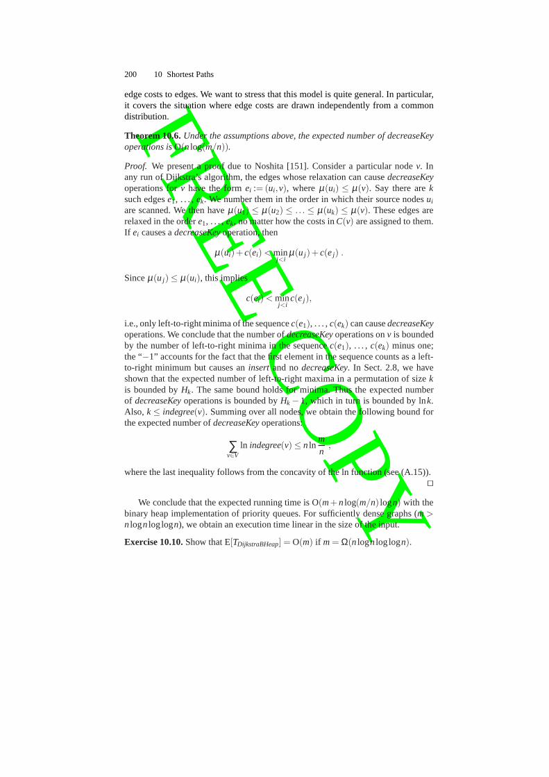
Theorem 10.6.Under the assumptions above, the expected number of decreaseKeyoperations isO(nlog(m/n)).

Proof. We present a proof due to Noshita [151]. Consider a particular nodev. Inany run of Dijkstra’s algorithm, the edges whose relaxationcan causedecreaseKeyoperations forv have the formei := (ui ,v), whereµ(ui) ≤ µ(v). Say there areksuch edgese1, . . . , ek. We number them in the order in which their source nodesui

are scanned. We then haveµ(u1) ≤ µ(u2) ≤ . . . ≤ µ(uk) ≤ µ(v). These edges arerelaxed in the ordere1, . . . ,ek, no matter how the costs inC(v) are assigned to them.If ei causes adecreaseKeyoperation, then

µ(ui)+c(ei) < minj<i

µ(u j)+c(ej) .

Sinceµ(u j) ≤ µ(ui), this implies

c(ei) < minj<i

c(ej),

i.e., only left-to-right minima of the sequencec(e1), . . . ,c(ek) can causedecreaseKeyoperations. We conclude that the number ofdecreaseKeyoperations onv is boundedby the number of left-to-right minima in the sequencec(e1), . . . , c(ek) minus one;the “−1” accounts for the fact that the first element in the sequencecounts as a left-to-right minimum but causes aninsert and nodecreaseKey. In Sect. 2.8, we haveshown that the expected number of left-to-right maxima in a permutation of sizekis bounded byHk. The same bound holds for minima. Thus the expected numberof decreaseKeyoperations is bounded byHk −1, which in turn is bounded by lnk.Also, k ≤ indegree(v). Summing over all nodes, we obtain the following bound forthe expected number ofdecreaseKeyoperations:

∑v∈V

ln indegree(v) ≤ nlnmn

,

where the last inequality follows from the concavity of the ln function (see (A.15)).⊓⊔

We conclude that the expected running time is O(m+nlog(m/n) logn) with thebinary heap implementation of priority queues. For sufficiently dense graphs (m>nlognlog logn), we obtain an execution time linear in the size of the input.

Exercise 10.10.Show that E[TDijkstraBHeap] = O(m) if m= Ω(nlognlog logn).

FRE

EC

OP

Y10.5 Monotone Integer Priority Queues 201

10.5 Monotone Integer Priority Queues

Dijkstra’s algorithm is designed to scan nodes in order of nondecreasing distancevalues. Hence, a monotone priority queue (see Chapter 6) suffices for its implemen-tation. It is not known whether monotonicity can be exploited in the case of generalreal edge costs. However, for integer edge costs, significant savings are possible. Wetherefore assume in this section that edge costs are integers in the range 0..C forsome integerC. C is assumed to be known when the queue is initialized.

Since a shortest path can consist of at mostn− 1 edges, the shortest-path dis-tances are at most(n− 1)C. The range of values in the queue at any one time iseven smaller. Letmin be the last value deleted from the queue (zero before the firstdeletion). Dijkstra’s algorithm maintains the invariant that all values in the queue arecontained inmin..min+C. The invariant certainly holds after the first insertion. AdeleteMinmay increasemin. Since all values in the queue are bounded byC plusthe old value ofmin, this is certainly true for the new value ofmin. Edge relaxationsinsert priorities of the formd[u]+c(e) = min+c(e) ∈ min..min+C.

10.5.1 Bucket Queues

A bucket queue is a circular arrayB of C+ 1 doubly linked lists (see Figs. 10.7and 3.8). We view the natural numbers as being wrapped aroundthe circular array;all integers of the formi +(C+1) j map to the indexi. A nodev∈ Q with tentativedistanced[v] is stored inB[d[v] mod(C+ 1)]. Since the priorities in the queue arealways inmin..min+C, all nodes in a bucket have thesamedistance value.

Initialization createsC + 1 empty lists. Aninsert(v) insertsv into B[d[v] modC+ 1]. A decreaseKey(v) removesv from the list containing it and insertsv intoB[d[v] modC+1]. Thus insert and decreaseKeytake constant time if buckets areimplemented as doubly linked lists.

A deleteMinfirst looks at bucketB[min modC+ 1]. If this bucket is empty, itincrementsmin and repeats. In this way, the total cost of alldeleteMinoperationsis O(n+nC) = O(nC), sincemin is incremented at mostnC times and at mostnelements are deleted from the queue. Plugging the operationcosts for the bucketqueue implementation with integer edge costs in 0..C into our general bound for thecost of Dijkstra’s algorithm, we obtain

TDijkstraBucket= O(m+nC) .

*Exercise 10.11 (Dinic’s refinement of bucket queues [57]).Assume that the edgecosts are positive real numbers in[cmin,cmax]. Explain how to find shortest paths intime O(m+ncmax/cmin). Hint: use buckets of widthcmin. Show that all nodes in thesmallest nonempty bucket haved[v] = µ(v).

10.5.2 *Radix Heaps

Radix heaps [9] improve on the bucket queue implementation by using buckets ofdifferent widths. Narrow buckets are used for tentative distances close tomin, and

FRE

EC

OP

Y202 10 Shortest Paths

b,30 30c,

e,33

d,31

a,29

f, 35

g,36

g,36 f, 35 e,33b,30 d,31 30c,a,29

01

23

456

7

89

min

−1

11101 11100 1111* 110** 10***

0 1 2 3

mod 10

Binary Radix Heap

content=

bucket queue withC = 9

4 = K

≥ 100000

〈(a,29),(b,30),(c,30),(d,31),(e,33),( f ,35),(g,36)〉 =

〈(a,11101),(b,11110),(c,11110),(d,11111),(e,100001),( f ,100011),(g,100100)〉

Fig. 10.7.Example of a bucket queue (upper part) and a radix heap (lower part). SinceC = 9,we haveK = 1+⌊logC⌋ = 4. The bit patterns in the buckets of the radix heap indicate the setof keys they can accommodate

wide buckets are used for tentative distances far away frommin. In this subsection,we shall show how this approach leads to a version of Dijkstra’s algorithm withrunning time

TDijkstraRadix:=O(m+nlogC) .

Radix heaps exploit the binary representation of tentativedistances. We needthe concept of themost significant distinguishing indexof two numbers. This is thelargest index where the binary representations differ, i.e., for numbersa andb withbinary representationsa= ∑i≥0 αi2i andb= ∑i≥0 βi2i , we define the most significantdistinguishing indexmsd(a,b) as the largesti with αi 6= βi , and let it be−1 if a = b.If a < b, thena has a zero bit in positioni = msd(a,b) andb has a one bit.

A radix heap consists of an array of bucketsB[−1], B[0], . . . , B[K], whereK =1+ ⌊logC⌋. The queue elements are distributed over the buckets according to thefollowing rule:

any queue elementv is stored in bucketB[i], wherei = min(msd(min,d[v]),K).

We refer to this rule as the bucket queue invariant. Figure 10.7 gives an example. Weremark that ifminhas a one bit in positioni for 0≤ i < K, the corresponding bucketB[i] is empty. This holds since anyd[v] with i = msd(min,d[v]) would have a zero bitin positioni and hence be smaller thanmin. But all keys in the queue are at least aslarge asmin.

How can we computei :=msd(a,b)? We first observe that fora 6= b, the bitwiseexclusive ORa⊕b of a andb has its most significant one in positioni and hencerepresents an integer whose value is at least 2i and less than 2i+1. Thusmsd(a,b) =

FRE

EC

OP

Y10.5 Monotone Integer Priority Queues 203

⌊log(a⊕b)⌋, since log(a⊕b) is a real number with its integer part equal toi and thefloor function extracts the integer part. Many processors support the computation ofmsdby machine instructions.3 Alternatively, we can use lookup tables or yet othersolutions. From now on, we shall assume thatmsdcan be evaluated in constant time.

We turn now to the queue operations. Initialization,insert, anddecreaseKeyworkcompletely analogously to bucket queues. The only difference is that bucket indicesare computed using the bucket queue invariant.

A deleteMinfirst finds the minimumi such thatB[i] is nonempty. Ifi = −1,an arbitrary element inB[−1] is removed and returned. Ifi ≥ 0, the bucketB[i] isscanned andmin is set to the smallest tentative distance contained in the bucket.Sincemin has changed, the bucket queue invariant needs to be restored. A crucialobservation for the efficiency of radix heaps is that only thenodes in bucketi areaffected. We shall discuss below how they are affected. Let us consider first thebucketsB[ j] with j 6= i. The bucketsB[ j] with j < i are empty. Ifi = K, there areno j ’s with j > K. If i < K, any keya in bucketB[ j] with j > i will still havemsd(a,min) = j, because the old and new values ofminagree at bit positions greaterthani.

What happens to the elements inB[i]? Its elements are moved to the appro-priate new bucket. Thus adeleteMintakes constant time ifi = −1 and takes timeO(i + |B[i]|) = O(K + |B[i]|) if i ≥ 0. Lemma 10.7 below shows that every node inbucketB[i] is moved to a bucket with a smaller index. This observation allows us toaccount for the cost of adeleteMinusing amortized analysis. As our unit of cost (onetoken), we shall use the time required to move one node between buckets.

We chargeK + 1 tokens for operationinsert(v) and associate theseK + 1 to-kens withv. These tokens pay for the moves ofv to lower-numbered buckets indeleteMinoperations. A node starts in some bucketj with j ≤ K, ends in bucket−1, and in between never moves back to a higher-numbered bucket. Observe that adecreaseKey(v) operation will also never move a node to a higher-numbered bucket.Hence, theK + 1 tokens can pay for all the node moves ofdeleteMinoperations.The remaining cost of adeleteMinis O(K) for finding a nonempty bucket. Withamortized costsK +1+O(1) = O(K) for an insertand O(1) for a decreaseKey, weobtain a total execution time of O(m+n · (K +K)) = O(m+nlogC) for Dijkstra’salgorithm, as claimed.

It remains to prove thatdeleteMinoperations move nodes to lower-numberedbuckets.

Lemma 10.7.Let i be minimal such that B[i] is nonempty and assume i≥ 0. Let minbe the smallest element in B[i]. Then msd(min,x) < i for all x ∈ B[i].

3 ⊕ is a direct machine instruction, and⌊logx⌋ is the exponent in the floating-point represen-tation ofx.

FRE

EC

OP

Y204 10 Shortest Paths

1

1

1

1

j 00

0

1

hCase i=K

mini 00

min

x

o

Casei<K

α

α

α

α

α

α

β

β

Fig. 10.8.The structure of the keys relevant to the proof of Lemma 10.7.In the proof, it isshown thatβ starts withj −K zeros

Proof. Observe first that the casex = min is easy, sincemsd(x,x) = −1 < i. For thenontrivial casex 6= min, we distinguish the subcasesi < K andi = K. Letmino be theold value ofmin. Figure 10.8 shows the structure of the relevant keys.

Casei < K. The most significant distinguishing index ofmino and anyx ∈ B[i] isi, i.e., mino has a zero in bit positioni, and allx ∈ B[i] have a one in bit positioni. They agree in all positions with an index larger thani. Thus the most significantdistinguishing index forminandx is smaller thani.

Case i = K. Consider anyx ∈ B[K]. Let j = msd(mino,min). Then j ≥ K, sincemin∈ B[K]. Let h = msd(min,x). We want to show thath < K. Let α comprise thebits in positions larger thanj in mino, and letA be the number obtained frommino bysetting the bits in positions 0 toj to zero. Thenα followed by j +1 zeros is the binaryrepresentation ofA. Since thej-th bit of mino is zero and that ofmin is one, we havemino < A+2 j andA+2 j ≤ min. Also,x≤ mino+C < A+2 j +C≤ A+2 j +2K . So

A+2 j ≤ min≤ x < A+2 j +2K,

and hence the binary representations ofmin and x consist ofα followed by a 1,followed by j −K zeros, followed by some bit string of lengthK. Thusmin andxagree in all bits with indexK or larger, and henceh < K.

In order to aid intuition, we give a second proof for the casei = K. We firstobserve that the binary representation ofmin starts withα followed by a one. Wenext observe thatx can be obtained frommino by adding someK-bit number. Sincemin≤ x, the final carry in this addition must run into positionj. Otherwise, thej-thbit of x would be zero and hencex < min. Sincemino has a zero in positionj, thecarry stops at positionj. We conclude that the binary representation ofx is equal toα followed by a 1, followed byj −K zeros, followed by someK-bit string. Sincemin≤ x, the j−K zeros must also be present in the binary representation ofmin. ⊓⊔

*Exercise 10.12.Radix heaps can also be based on number representations withbaseb for anyb ≥ 2. In this situation we have bucketsB[i, j] for i = −1,0,1, . . . ,K and0≤ j ≤ b, whereK = 1+ ⌊logC/ logb⌋. An unscanned reached nodex is stored inbucketB[i, j ] if msd(min,d[x]) = i and thei-th digit of d[x] is equal to j. We alsostore, for eachi, the number of nodes contained in the buckets∪ jB[i, j ]. Discussthe implementation of the priority queue operations and show that a shortest-path

FRE

EC

OP

Y10.5 Monotone Integer Priority Queues 205

algorithm with running time O(m+n(b+ logC/ logb)) results. What is the optimalchoice ofb?

If the edge costs are random integers in the range 0..C, a small change to Dijk-stra’s algorithm with radix heaps guarantees linear running time [139, 76]. For everynodev, let cin

min(v) denote the minimum cost of an incoming edge. We divideQ intotwo parts, a setF which contains unscanned nodes whose tentative-distance labelis known to be equal to their exact distance froms, and a partB which contains allother reached unscanned nodes.B is organized as a radix heap. We also maintain avaluemin. We scan nodes as follows.

WhenF is nonempty, an arbitrary node inF is removed and the outgoing edgesare relaxed. WhenF is empty, the minimum node is selected fromB andmin is setto its distance label. When a node is selected fromB, the nodes in the first nonemptybucketB[i] are redistributed ifi ≥ 0. There is a small change in the redistributionprocess. When a nodev is to be moved, andd[v] ≤ min+ cin

min(v), we movev to F .Observe that any future relaxation of an edge intov cannot decreased[v], and henced[v] is known to be exact at this point.

We call this algorithm ALD (average-case linear Dijkstra).The algorithm ALDis correct, since it is still true thatd[v] = µ(v) whenv is scanned. For nodes removedfrom F , this was argued in the previous paragraph, and for nodes removed fromB,this follows from the fact that they have the smallest tentative distance among allunscanned reached nodes.

Theorem 10.8.Let G be an arbitrary graph and let c be a random function from Eto 0..C. The algorithm ALD then solves the single-source problem in expected timeO(m+n).

Proof. We still need to argue the bound on the running time. To do this, we modifythe amortized analysis of plain radix heaps. As before, nodes start out inB[K]. Whena nodev has been moved to a new bucket but not yet toF , d[v] > min+cin

min(v), andhencev is moved to a bucketB[i] with i ≥ logcin

min(v). Hence, it suffices ifinsertpaysK − logcin

min(v)+1 tokens into the account for nodev in order to cover all costs dueto decreaseKeyanddeleteMinoperations operating onv. Summing over all nodes,we obtain a total payment of

∑v

(K − logcinmin(v)+1) = n+∑

v(K − logcin

min(v)) .

We need to estimate this sum. For each vertex, we have one incoming edge contribut-ing to this sum. We therefore bound the sum from above if we sumover all edges,i.e.,

∑v

(K − logcinmin(v)) ≤ ∑

e(K− logc(e)) .

K− logc(e) is the number of leading zeros in the binary representation of c(e) whenwritten as aK-bit number. Our edge costs are uniform random numbers in 0..C, andK = 1+ ⌊logC⌋. Thus prob(K− logc(e) = i) = 2−i . Using (A.14), we conclude that

FRE

EC

OP

Y206 10 Shortest Paths

E

[

∑e

(k− logc(e))

]

= ∑e

∑i≥0

i2−i = O(m) .

Thus the total expected cost of thedeleteMinanddecreaseKeyoperations is O(m+n).The time spent outside these operations is also O(m+n). ⊓⊔

It is a little odd that the maximum edge costC appears in the premise but not inthe conclusion of Theorem 10.8. Indeed, it can be shown that asimilar result holdsfor random real-valued edge costs.

**Exercise 10.13.Explain how to adapt the algorithm ALD to the case wherec isa random function fromE to the real interval(0,1]. The expected time should stillbe O(m+n). What assumptions do you need about the representation of edge costsand about the machine instructions available? Hint: you mayfirst want to solve Ex-ercise 10.11. The narrowest bucket should have a width of mine∈E c(e). Subsequentbuckets have geometrically growing widths.

10.6 Arbitrary Edge Costs (Bellman–Ford Algorithm)

For acyclic graphs and for nonnegative edge costs, we got away with m edge re-laxations. For arbitrary edge costs, no such result is known. However, it is easy toguarantee the correctness criterion of Lemma 10.3 using O(n ·m) edge relaxations:the Bellman–Ford algorithm [18, 63] given in Fig. 10.9 performsn− 1 rounds. Ineach round, it relaxes all edges. Since simple paths consistof at mostn−1 edges,every shortest path is a subsequence of this sequence of relaxations. Thus, after therelaxations are completed, we haved[v] = µ(v) for all v with −∞ < d[v] < ∞, byLemma 10.3. Moreover,parentencodes the shortest paths to these nodes. Nodesvunreachable fromswill still have d[v] = ∞, as desired.

It is not so obvious how to find the nodesv with µ(v) = −∞. Consider any edgee = (u,v) with d[u] + c(e) < d[v] after the relaxations are completed. We can setd[v] :=−∞ because if there were a shortest path froms to v, we would have found itby now and relaxingewould not lead to shorter distances anymore. We can now alsosetd[w] = −∞ for all nodesw reachable fromv. The pseudocode implements thisapproach using a recursive functioninfect(v). It sets thed-value ofv and all nodesreachable from it to−∞. If infect reaches a nodew that already hasd[w] = −∞,it breaks the recursion because previous executions ofinfect have already exploredall nodes reachable fromw. If d[v] is not set to−∞ during postprocessing, we haved[x]+c(e)≥ d[y] for any edgee= (x,y) on any pathp froms to v. Thusd[s]+c(p)≥d[v] for any pathp from s to v, and henced[v]≤ µ(v). We conclude thatd[v] = µ(v).

Exercise 10.14.Show that the postprocessing runs in time O(m). Hint: relateinfectto DFS.

Exercise 10.15.Someone proposes an alternative postprocessing algorithm: setd[v]to−∞ for all nodesv for which following parents does not lead tos. Give an examplewhere this method overlooks a node withµ(v) = −∞.

FRE

EC

OP

Y10.7 All-Pairs Shortest Paths and Node Potentials 207

Function BellmanFord(s : NodeId) : NodeArray×NodeArrayd = 〈∞, . . . ,∞〉 : NodeArrayof R∪−∞,∞ // distance from rootparent =〈⊥, . . . ,⊥〉 : NodeArrayof NodeIdd[s] :=0; parent[s] := s // self-loop signals rootfor i :=1 to n−1 do

forall e∈ E do relax(e) // roundi

forall e= (u,v) ∈ E do // postprocessingif d[u]+c(e) < d[v] then infect(v)

return (d,parent)

Procedure infect(v)if d[v] > −∞ then

d[v] :=−∞foreach (v,w) ∈ E do infect(w)

Fig. 10.9.The Bellman–Ford algorithm for shortest paths in arbitrarygraphs

Exercise 10.16 (arbitrage). Consider a set of currenciesC with an exchange rateof r i j between currenciesi and j (you obtainr i j units of currencyj for one unit ofcurrencyi). A currency arbitrageis possible if there is a sequence of elementarycurrency exchange actions (transactions) that starts with one unit of a currency andends with more than one unit of the same currency. (a) Show howto find out whethera matrix of exchange rates admits currency arbitrage. Hint:log(xy)= logx+ logy. (b)Refine your algorithm so that it outputs a sequence of exchange steps that maximizesthe average profitper transaction.

Section 10.10 outlines further refinements of the Bellman–Ford algorithm thatare necessary for good performance in practice.

10.7 All-Pairs Shortest Paths and Node Potentials

The all-pairs problem is tantamount ton single-source problems and hence can besolved in time O

(n2m

). A considerable improvement is possible. We shall show

that it suffices to solve one general single-source problem plus n single-sourceproblems with nonnegative edge costs. In this way, we obtaina running time ofO(nm+n(m+nlogn)) = O

(nm+n2 logn

). We need the concept of node potentials.

A (node) potential functionassigns a numberpot(v) to each nodev. For an edgee= (v,w), we define itsreduced costc(e) as

c(e) = pot(v)+c(e)−pot(w) .

Lemma 10.9. Let p and q be paths from v to w. Thenc(p) = pot(v)+c(p)−pot(w)andc(p)≤ c(q) iff c(p)≤ c(q). In particular, the shortest paths with respect toc arethe same as those with respect to c.

FRE

EC

OP

Y208 10 Shortest Paths

All-Pairs Shortest Paths in the Absence of Negative Cyclesadd a new nodesand zero length edges(s,v) for all v // no new cycles, time O(m)computeµ(v) for all v with Bellman–Ford // time O(nm)setpot(v) = µ(v) and compute reduced costs ¯c(e) for e∈ E // time O(m)forall nodesx do // time O(n(m+nlogn))

use Dijkstra’s algorithm to compute the reduced shortest-path distancesµ(x,v)using sourcex and the reduced edge costs ¯c

// translate distances back to original cost function // time O(m)forall e= (v,w) ∈V ×V do µ(v,w) := µ(v,w)+pot(w)−pot(v) // use Lemma 10.9

Fig. 10.10.Algorithm for all-pairs shortest paths in the absence of negative cycles

Proof. The second and the third claim follow from the first. For the first claim, letp = 〈e0, . . . ,ek−1〉, whereei = (vi ,vi+1), v = v0, andw = vk. Then

c(p) =k−1

∑i=0

c(ei) = ∑0≤i<k

(pot(vi)+c(ei)−pot(vi+1))

= pot(v0)+ ∑0≤i<k

c(ei)−pot(vk) = pot(v0)+c(p)−pot(vk) . ⊓⊔

Exercise 10.17.Node potentials can be used to generate graphs with negativeedgecosts but no negative cycles: generate a (random) graph, assign to every edgee a(random) nonnegative costc(e), assign to every nodev a (random) potentialpot(v),and set the cost ofe = (u,v) to c(e) = pot(u)+ c(e)− pot(v). Show that this ruledoes not generate negative cycles.

Lemma 10.10.Assume that G has no negative cycles and that all nodes can bereached from s. Let pot(v) = µ(v) for v∈V. With these node potentials, the reducededge costs are nonnegative.

Proof. Since all nodes are reachable froms and since there are no negative cycles,µ(v)∈R for all v. Thus the reduced costs are well defined. Consider an arbitrary edgee= (v,w). We haveµ(v)+c(e)≥ µ(w), and thus ¯c(e) = µ(v)+c(e)−µ(w)≥ 0. ⊓⊔

Theorem 10.11.The all-pairs shortest-path problem for a graph without negativecycles can be solved in timeO

(nm+n2 logn

).

Proof. The algorithm is shown in Fig. 10.10. We add an auxiliary nodes and zero-cost edges(s,v) for all nodes of the graph. This does not create negative cyclesand does not changeµ(v,w) for any of the existing nodes. Then we solve the single-source problem for the sources, and setpot(v) = µ(v) for all v. Next we compute thereduced costs and then solve the single-source problem for each nodex by means ofDijkstra’s algorithm. Finally, we translate the computed distances back to the originalcost function. The computation of the potentials takes timeO(nm), and then shortest-path calculations take time O(n(m+nlogn)). The preprocessing and postprocessingtake linear time. ⊓⊔

FRE

EC

OP

Y10.8 Shortest-Path Queries 209

The assumption thatG has no negative cycles can be removed [133].

Exercise 10.18.Thediameter Dof a graphG is defined as the largest distance be-tween any two of its nodes. We can easily compute it using an all-pairs compu-tation. Now we want to consider ways toapproximatethe diameter of a stronglyconnected graph using a constant number of single-source computations. (a) Forany starting nodes, let D′(s) := maxu∈V µ(u). Show thatD′(s) ≤ D ≤ 2D′(s) forundirected graphs. Also, show that no such relation holds for directed graphs. LetD′′(s) :=maxu∈V µ(u,s). Show that max(D′(s),D′′(s)) ≤D ≤ D′(s)+D′′(s) for bothundirected and directed graphs. (b) How should a graph be represented to supportboth forward and backward search? (c) Can you improve the approximation by con-sidering more than one nodes?

10.8 Shortest-Path Queries

We are often interested in the shortest path from a specific source nodes to a spe-cific target nodet; route planning in a traffic network is one such scenario. We shallexplain some techniques for solving suchshortest-path queriesefficiently and arguefor their usefulness for the route-planning application.

We start with a technique calledearly stopping. We run Dijkstra’s algorithm tofind shortest paths starting ats. We stop the search as soon ast is removed from thepriority queue, because at this point in time the shortest path tot is known. This helpsexcept in the unfortunate case wheret is the node farthest froms. On average, earlystopping saves a factor of two in scanned nodes in any application. In practical routeplanning, early stopping saves much more because modern carnavigation systemshave a map of an entire continent but are mostly used for distances up to a fewhundred kilometers.

Another simple and general heuristic isbidirectional search, from s forward andfrom t backward until the search frontiers meet. More precisely, we run two copiesof Dijkstra’s algorithm side by side, one starting froms and one starting fromt (andrunning on the reversed graph). The two copies have their ownqueues, sayQs andQt , respectively. We grow the search regions at about the same speed, for exampleby removing a node fromQs if min Qs ≤ minQt and a node fromQt otherwise.

It is tempting to stop the search once the first nodeu has been removed fromboth queues, and to claim thatµ(t) = µ(s,u)+ µ(u,t). Observe that execution ofDijkstra’s algorithm on the reversed graph with a starting nodet determinesµ(u,t).This is not quite correct, but almost so.

Exercise 10.19.Give an example whereu is not on the shortest path froms to t.

However, we have collected enough information once some node u has beenremoved from both queues. Letds anddt denote the tentative-distance labels at thetime of termination in the runs with sources and sourcet, respectively. We showthat µ(t) < µ(s,u) + µ(u,t) implies the existence of a nodev ∈ Qs with µ(t) =ds[v]+dt[v].

FRE

EC

OP

Y210 10 Shortest Paths

Let p = 〈s= v0, . . . ,vi ,vi+1, . . . ,vk = t〉 be a shortest path froms to t. Let i bemaximal such thatvi has been removed fromQs. Thends[vi+1] = µ(s,vi+1) andvi+1 ∈ Qs when the search stops. Also,µ(s,u)≤ µ(s,vi+1), sinceu has already beenremoved fromQs, butvi+1 has not. Next, observe that

µ(s,vi+1)+ µ(vi+1,t) = c(p) < µ(s,u)+ µ(u,t) ,

sincep is a shortest path froms to t. By subtractingµ(s,vi+1), we obtain

µ(vi+1,t) < µ(s,u)− µ(s,vi+1)︸ ︷︷ ︸

≤0

+µ(u,t) ≤ µ(u,t)

and hence, sinceu has been scanned fromt, vi+1 must also have been scanned fromt, i.e.,dt [vi+1] = µ(vi+1,t) when the search stops. So we can determine the shortestdistance froms to t by inspecting not only the first node removed from both queues,but also all nodes in, say,Qs. We iterate over all such nodesv and determine theminimum value ofds[v]+dt [v].

Dijkstra’s algorithm scans nodes in order of increasing distance from the source.In other words, it grows a circle centered on the source node.The circle is defined bythe shortest-path metric in the graph. In the route-planning application for a road net-work, we may also consider geometric circles centered on thesource and argue thatshortest-path circles and geometric circles are about the same. We can then estimatethe speedup obtained by bidirectional search using the following heuristic argument:a circle of a certain diameter has twice the area of two circles of half the diameter.We could thus hope that bidirectional search will save a factor of two compared withunidirectional search.

Exercise 10.20 (bidirectional search).(a) Consider bidirectional search in a gridgraph with unit edge weights. How much does it save over unidirectional search? (*b)Try to find a family of graphs where bidirectional search visits exponentially fewernodes on average than does unidirectional search. Hint: consider random graphs orhypercubes. (c) Give an example where bidirectional searchin a real road networktakeslonger than unidirectional search. Hint: consider a densely inhabitated citywith sparsely populated surroundings. (d) Design a strategy for switching betweenforward and backward search such that bidirectional searchwill neverinspect morethan twice as many nodes as unidirectional search.

We shall next describe two techniques that are more complex and less generallyapplicable: however, if they are applicable, they usually result in larger savings. Bothtechniques mimic human behavior in route planning.

10.8.1 Goal-Directed Search

The idea is to bias the search space such that Dijkstra’s algorithm does not growa disk but a region protruding toward the target; see Fig. 10.11. Assume we knowa function f : V → R that estimates the distance to the target, i.e.,f (v) estimates

FRE

EC

OP

Y10.8 Shortest-Path Queries 211

µ(v,t) for all nodesv. We use the estimates to modify the distance function. Foreache = (u,v), let4 c(e) = c(e) + f (v)− f (u). We run Dijkstra’s algorithm withthe modified distance function. We know already that node potentials do not changeshortest paths, and hence correctness is preserved. Tentative distances are related viad[v] = d[v] + f (v)− f (s). An alternative view of this modification is that we runDijkstra’s algorithm with the original distance function but remove the node withminimal valued[v]+ f (v) from the queue. The algorithm just described is known asA∗-search.

ss tt

Fig. 10.11. The standard Dijkstra search grows a circular region centered on the source; goal-directed search grows a region protruding toward the target

Before we state requirements on the estimatef , let us see one specific example.Assume, in a thought experiment, thatf (v) = µ(v,t). Thenc(e) = c(e)+ µ(v,t)−µ(u,t) and hence edges on a shortest path froms to t have a modified cost equal tozero and all other edges have a positive cost. Thus Dijkstra’s algorithm only followsshortest paths, without looking left or right.

The function f must have certain properties to be useful. First, we want themodified distances to be nonnegative. So, we needc(e)+ f (v) ≥ f (u) for all edgese= (u,v). In other words, our estimate of the distance fromu should be at most ourestimate of the distance fromv plus the cost of going fromu to v. This property iscalled consistency of estimates. We also want to be able to stop the search whentis removed from the queue. This works iff is a lower bound on the distance to thetarget, i.e.,f (v) ≤ µ(v,t) for all v ∈ V. Then f (t) = 0. Consider the point in timewhent is removed from the queue, and letp be any path froms to t. If all edges ofphave been relaxed at termination,d[t]≤ c(p). If not all edges ofp have been relaxedat termination, there is a nodev on p that is contained in the queue at termination.Thend(t)+ f (t) ≤ d(v)+ f (v), sincet was removed from the queue butv was not,and hence

d[t] = d[t]+ f (t)≤ d[v]+ f (v) ≤ d[v]+ µ(v,t)≤ c(p) .

In either case, we haved[t] ≤ c(p), and hence the shortest distance froms to t isknown as soon ast is removed from the queue.

What is a good heuristic function for route planning in a roadnetwork? Routeplanners often give a choice betweenshortestand fastestconnections. In the case

4 In Sect. 10.7, we added the potential of the source and subtracted the potential of the target.We do exactly the opposite now. The reason for changing the sign convention is that inLemma 10.10, we usedµ(s,v) as the node potential. Now,f estimatesµ(v,t).

FRE

EC

OP

Y212 10 Shortest Paths

of shortest paths, a feasible lower boundf (v) is the straight-line distance betweenvandt. Speedups by a factor of roughly four are reported in the literature. For fastestpaths, we may use the geometric distance divided by the speedassumed for the bestkind of road. This estimate is extremely optimistic, since targets are frequently in thecenter of a town, and hence no good speedups have been reported. More sophisticatedmethods for computing lower bounds are known; we refer the reader to [77] for athorough discussion.

10.8.2 Hierarchy

Road networks usually contain a hierarchy of roads: throughways, state roads, countyroads, city roads, and so on. Average speeds are usually higher on roads of higherstatus, and therefore the fastest routes frequently followthe pattern that one startson a road of low status, changes several times to roads of higher status, drives thelargest fraction of the path on a road of high status, and finally changes down tolower-status roads near the target. A heuristic approach may therefore restrict thesearch to high-status roads except for suitably chosen neighborhoods of the sourceand target. Observe, however, that the choice of neighborhood is nonobvious, andthat this heuristic sacrifices optimality. You may be able tothink of an example fromyour driving experience where shortcuts over small roads are required even far awayfrom the source and target. Exactness can be combined with the idea of hierarchies ifthe hierarchy is defined algorithmically and is not taken from the official classifica-tion of roads. We now outline one such approach [165], calledhighway hierarchies.It first defines a notion of locality, say anything within a distance of 10 km fromeither the source or the target. An edge(u,v) ∈ E is ahighway edgewith respect tothis notion of locality if there is a source nodes and a target nodet such that(u,v)is on the fastest path froms to t, v is not within the local search radius ofs, anduis not within the local (backward) search radius oft. The resulting network is calledthehighway network. It usually has many vertices of degree two. Think of a fast roadto which a slow road connects. The slow road is not used on any fastest path outsidethe local region of a nearby source or nearby target, and hence will not be in thehighway network. Thus the intersection will have degree three in the original roadnetwork, but will have degree two in the highway network. Twoedges joined by adegree-two node may be collapsed into a single edge. In this way, thecore of thehighway network is determined. Iterating this procedure offinding a highway net-work and contracting degree-two nodes leads to a hierarchy of roads. For example,in the case of the road networks of Europe and North America, ahierarchy of upto ten levels resulted. Route planning using the resulting highway hierarchy can beseveral thousand times faster than Dijkstra’s algorithm.

10.8.3 Transit Node Routing

Using another observation from daily life, we can get even faster [15]. When youdrive to somewhere “far away”, you will leave your current location via one of onlya few “important” traffic junctions. It turns out that in real-world road networks about

FRE

EC

OP

Y10.9 Implementation Notes 213

Fig. 10.12.Finding the optimal travel time between two points (the flags) somewhere be-tween Saarbrücken and Karlsruhe amounts to retrieving the 2×4 access nodes(diamonds),performing 16 table lookups between all pairs of access nodes, and checking that the two disksdefining thelocality filter do not overlap. The small squares indicate further transit nodes

99% of all quickest paths go through about O(√

n) importanttransit nodesthat can beautomatically selected, for example using highway hierarchies. Moreover, for eachparticular source or target node, all long-distance connections go through one ofabout ten of these transit nodes – theaccess nodes. During preprocessing, we com-pute a complete distance table between the transit nodes, and the distances from allnodes to their access nodes. Now, suppose we have a way to tellthat a sources anda targett are sufficiently far apart.5 There must then be access nodesas andat suchthat µ(t) = µ(as)+ µ(as,at)+ µ(at ,t). All these distances have been precomputedand there are only about ten candidates foras and forat , respectively, i.e., we need(only) about 100 accesses to the distance table. This can be more than 1 000 000times faster than Dijkstra’s algorithm. Local queries can be answered using someother technique that will profit from the closeness of the source and target. We canalso cover local queries using additional precomputed tables with more local infor-mation. Figure 10.12 from [15] gives an example.

10.9 Implementation Notes

Shortest-path algorithms work over the set of extended reals R∪ +∞,−∞. Wemay ignore−∞, since it is needed only in the presence of negative cycles and, eventhere, it is needed only for the output; see Sect. 10.6. We canalso get rid of+∞ bynoting thatparent(v) = ⊥ iff d[v] = +∞, i.e., whenparent(v) = ⊥, we assume thatd[v] = +∞ and ignore the number stored ind[v].

5 We may need additional preprocessing to decide this.

FRE

EC

OP

Y214 10 Shortest Paths

A refined implementation of the Bellman–Ford algorithm [187, 131] explicitlymaintains a current approximationT of the shortest-path tree. Nodes still to bescanned in the current iteration of the main loop are stored in a setQ. Considerthe relaxation of an edgee= (u,v) that reducesd[v]. All descendants ofv in T willsubsequently receive a newd-value. Hence, there is no reason to scan these nodeswith their currentd-values and one may remove them fromQ andT. Furthermore,negative cycles can be detected by checking whetherv is an ancestor ofu in T.

10.9.1 C++

LEDA [118] has a special priority queue classnode_pq that implements priorityqueues of graph nodes. Both LEDA and the Boost graph library [27] have imple-mentations of the Dijkstra and Bellman–Ford algorithms andof the algorithms foracyclic graphs and the all-pairs problem. There is a graph iterator based on Dijkstra’salgorithm that allows more flexible control of the search process. For example, onecan use it to search until a given set of target nodes has been found. LEDA also pro-vides a function that verifies the correctness of distance functions (see Exercise 10.8).

10.9.2 Java

JDSL [78] provides Dijkstra’s algorithm for integer edge costs. This implementationallows detailed control over the search similarly to the graph iterators of LEDA andBoost.

10.10 Historical Notes and Further Findings

Dijkstra [56], Bellman [18], and Ford [63] found their algorithms in the 1950s. Theoriginal version of Dijkstra’s algorithm had a running timeO

(m+n2

)and there

is a long history of improvements. Most of these improvements result from betterdata structures for priority queues. We have discussed binary heaps [208], Fibonacciheaps [68], bucket heaps [52], and radix heaps [9]. Experimental comparisons canbe found in [40, 131]. For integer keys, radix heaps are not the end of the story. Thebest theoretical result is O(m+nloglogn) time [194]. Interestingly, forundirectedgraphs, linear time can be achieved [190]. The latter algorithm still scans nodes oneafter the other, but not in the same order as in Dijkstra’s algorithm.

Meyer [139] gave the first shortest-path algorithm with linear average-case run-ning time. The algorithm ALD was found by Goldberg [76]. For graphs with boundeddegree, the∆ -stepping algorithm [140] is even simpler. This uses bucketqueues andalso yields a good parallel algorithm for graphs with bounded degree and small di-ameter.

Integrality of edge costs is also of use when negative edge costs are allowed.If all edge costs are integers greater than−N, a scaling algorithmachieves a timeO(m

√nlogN) [75].

FRE

EC

OP

Y10.10 Historical Notes and Further Findings 215

In Sect. 10.8, we outlined a small number of speedup techniques for route plan-ning. Many other techniques exist. In particular, we have not done justice to ad-vanced goal-directed techniques, combinations of different techniques, etc. Recentoverviews can be found in [166, 173]. Theoretical performance guarantees beyondDijkstra’s algorithm are more difficult to achieve. Positive results exist for specialfamilies of graphs such as planar graphs and when approximate shortest paths suf-fice [60, 195, 192].

There is a generalization of the shortest-path problem thatconsiders several costfunctions at once. For example, your grandfather might wantto know the fastestroute for visiting you but he only wants routes where he does not need to refuel hiscar, or you may want to know the fastest route subject to the condition that the roadtoll does not exceed a certain limit. Constrained shortest-path problems are discussedin [86, 135].

Shortest paths can also be computed in geometric settings. In particular, thereis an interesting connection to optics. Different materials have different refractiveindices, which are related to the speed of light in the material. Astonishingly, thelaws of optics dictate that a ray of light always travels along a shortest path.

Exercise 10.21.An ordered semigroup is a setS together with an associative andcommutative operation+, a neutral element 0, and a linear ordering≤ such that forall x, y, andz, x ≤ y impliesx+ z≤ y+ z. Which of the algorithms of this chapterwork when the edge weights are from an ordered semigroup? Which of them workunder the additional assumption that 0≤ x for all x?

FRE

EC

OP

Y