Embed Size (px)
Citation preview

10Retaining Walls: Analysis and Design
Alaa Ashmawy
CONTENTS10.1 Introduction ................................................................................................................... 42710.2 Lateral Earth Pressure.................................................................................................. 42910.3 Basic Design Principles................................................................................................ 436
10.3.1 Effect of Water Table...................................................................................... 43810.3.2 Effect of Compaction on Nonyielding Walls ............................................. 439
10.4 Gravity Walls................................................................................................................. 43910.5 Cantilever Walls............................................................................................................ 44610.6 MSE Walls ...................................................................................................................... 449
10.6.1 Internal Stability Analysis and Design........................................................ 45010.6.2 Reinforced Earth Walls .................................................................................. 45210.6.3 Geogrid-Reinforced Walls ............................................................................. 45410.6.4 Geotextile-Reinforced Walls.......................................................................... 454
10.7 Sheet-Pile and Tie-Back Anchored Walls ................................................................. 45510.7.1 Cantilever Sheet Piles..................................................................................... 45510.7.2 Anchored Sheet Piles...................................................................................... 458
10.7.2.1 Redundancy in Design .................................................................. 46010.7.3 Braced Excavations......................................................................................... 46010.7.4 Tie-Back Anchored Walls .............................................................................. 461
10.8 Soil Nail Systems .......................................................................................................... 46210.9 Drainage Considerations ............................................................................................. 46310.10 Deformation Analysis .................................................................................................. 46410.11 Performance under Seismic Loads ............................................................................ 46510.12 Additional Examples.................................................................................................... 466Glossary....................................................................................................................................... 482References ................................................................................................................................... 482
10.1 Introduction
Retaining walls are soil-structure systems intended to support earth backfills. Construc-tion of retaining walls is typically motivated by the need to eliminate slopes in roadwidening projects, to support bridges and similar overpass and underpass elements, or toprovide a level ground for shallow foundations. Retaining walls belong to a broader classof civil engineering structures, earth retaining structures, which also encompass temporarysupport elements such as sheet-pile walls, concrete slurry walls, and soil nails. Evidence
Gunaratne / The Foundation Engineering Handbook 1159_C010 Final Proof page 427 22.11.2005 2:56am
427
© 2006 by Taylor & Francis Group, LLC

of stone blocks and rockfill retaining walls is found at archeological sites around theworld. The western (wailing) wall in Jerusalem was built by King Herod as a retainingwall for the city, and the hanging gardens of Babylon are believed to have been steppedterraces supported by brick and stone walls.
Retaining walls have traditionally been constructed with plain or reinforced concrete,with the purpose of sustaining the soil pressure arising from the backfill. From an analysisand design standpoint, classical references categorize such walls into two types: gravitywalls and cantilever walls (Figure 10.1). The basic difference lies in the mechanisms andforces contributing to the wall stability; gravity walls rely on their own weight to providestatic equilibrium while cantilever walls derive a portion of their stabilizing forces andmoments from the backfill soil above the heel. From a construction standpoint, gravitywalls are typically made of plain (unreinforced) concrete or stone blocks, whereas canti-lever walls require the use of steel reinforcement to resist the large moments and shearstresses.
With the advent of reinforced earth technologies in the 1960s and geosynthetic mater-ials in the 1980s, gravity and cantilever walls are becoming largely obsolete. New tech-nologies such as mechanically stabilized earth (MSE) walls and soil nailing are becomingincreasingly popular due to their high efficiency, adaptability, and low cost. Figure 10.2shows typical cross sections in such earth retaining structures. Where larger and deeper
structures of choice. Although such integrated soil-inclusion systems have only begun tobe used in conventional civil engineering projects in recent years, the concept of soil
(a)
Backfill
Toe Heel
Backfill
(b)
FIGURE 10.1Conventional types of retaining walls: (a) gravity, (b) cantilever.
(a) (b)
FIGURE 10.2Cross section in (a) mechanically stabilized earth (MSE) wall and (b) soil-nailed wall.
Gunaratne / The Foundation Engineering Handbook 1159_C010 Final Proof page 428 22.11.2005 2:56am
428 The Foundation Engineering Handbook
© 2006 by Taylor & Francis Group, LLC
excavations are needed, sheet piles and tie-back anchored walls (Figure 10.3) are the

reinforcement has surprisingly been around for thousands of years. The ‘‘ziggurats’’ builtby the Babylonians, in what is modern day Iraq, were constructed from an outer wall offired brick, with the inside filled with clay reinforced with cedar beams. Despite the lowdurability of the bricks and clay, archeological remains of many of the ziggurats are still inexistence today, which reflects the high strength and durability of such systems.
The migration to MSE systems was initiated by the introduction of Reinforced Earth1, aproprietary technology that relies on reinforcing the backfill with galvanized steel strips.Since then, a broad range of similar technologies have emerged, relying on the samereinforcement mechanisms while utilizing other types of materials. The basic idea is toreinforce the soil with horizontal inclusions that extend back into the earth fill to form amonolithic mass that acts as a self-contained earth support system. Today, reinforcementelements include products ranging from natural fibers (e.g., coir and bamboo) to geosyn-thetics (e.g., geogrids and geotextiles). With progress made over the past decades inpolymer science and engineering, new species of polymers have become available thatexhibit relatively high strength and modulus, and excellent durability. As a result, MSEwalls, specifically those reinforced with geosynthetics, have become increasingly popularin transportation and geotechnical earthworks such as slope stabilization, highway ex-pansion, and, more recently, bridge abutments. Such bridge abutments can supporthigher surcharges, and loads concentrated near the facing of the wall.
10.2 Lateral Earth Pressure
In order to design earth retaining structures, it is necessary to have a thorough under-standing of lateral earth pressure concepts and theory. Although a comprehensive reviewof lateral earth pressure theories is beyond the scope of this chapter, we will present anoverview of the classical and commonly accepted theories. Because soils possess shearstrength, the magnitude of stress acting at a point may be different depending on thedirection. For instance, the horizontal pressure at a point within a soil mass is typicallydifferent from the vertical pressure. This is unlike fluids, where the pressure at a point is
0h
and the vertical effective stress, s0v is known as the coefficient of lateral earth pressure, K.
(a) (b)
FIGURE 10.3Alternative earth retaining systems: (a) sheet pile with a tie-back anchor, (b) tie-back anchored retaining wall.
Gunaratne / The Foundation Engineering Handbook 1159_C010 Final Proof page 429 22.11.2005 2:56am
Retaining Walls: Analysis and Design 429
© 2006 by Taylor & Francis Group, LLC
independent of direction (Figure 10.4). The ratio between horizontal effective stress, s ,

K ¼ s0hs0v
(10:1)
Typically, vertical stresses in a soil mass can be reliably calculated by multiplying the unitweight of the soil by the depth. In contrast, the horizontal stresses cannot be accuratelypredicted. The magnitude of the coefficient of lateral earth pressure depends not only onthe soil physical properties, but also on construction or deposition processes, stresshistory, and time among others. For a given vertical stress value, the ability of a soil toresist shear stresses results in a range of possible horizontal stresses (range of K values)where the soil remains stable. From a retaining earth structures design perspective, twolimits or conditions exist where the soil fails: active and passive. The correspondingcoefficients of lateral earth pressure are denoted Ka and Kp, respectively. Under ‘‘natural’’in situ conditions, the actual value of the lateral earth pressure coefficient is known as thecoefficient of lateral earth pressure at rest, K0.
According to Rankine’s (1857) theory, an active lateral earth pressure condition occurswhen the horizontal stress, s0h, decreases to the minimum possible value required for soilstability. In contrast, a passive condition takes place when s0h increases to a point wherethe soil fails due to excessive lateral compression. Figure 10.5 shows practical situationswhere active and passive failures may occur. To further illustrate the relationship be-tween the coefficient of lateral earth pressure and the soil’s shear strength, we consider
s h ≠ s v
s
s
s v
FIGURE 10.4Illustration of the concept of lateral earth pressure. The diagram to the left shows a difference between verticaland horizontal earth pressures (sv 6¼ sh). The diagram to the right illustrates an equal fluid pressure in alldirections.
Wallmovement
Wallmovement
Activ
e fa
ilure
pla
ne
Passive failure plane
(a) (b)
FIGURE 10.5Idealized lateral earth pressure conditions leading to failure due to (a) active and (b) passive earth pressure.
Gunaratne / The Foundation Engineering Handbook 1159_C010 Final Proof page 430 22.11.2005 2:56am
430 The Foundation Engineering Handbook
© 2006 by Taylor & Francis Group, LLC
the retaining wall shown in Figure 10.6. Assuming the friction between the soil and the

wall to be negligible, the vertical effective stress, s0v, at a depth z behind the wall is equalto gz. It follows that the horizontal effective stress is equal to Ks0v (Equation 10.1). Underat-rest conditions, the soil is far from failure, and the stress condition is represented inMohr’s stress space by circle A. Here, the coefficient of earth pressure at rest, K0, is equalto the ratio between s0h0 and s0v. Next, we assume that the wall ‘‘deforms’’ or moves awayfrom the backfill, thereby gradually reducing the horizontal pressure. Throughout thisprocess, the vertical pressure remains constant (s0v ¼ gz) since no changes are made invertical loading conditions. The horizontal stress may be reduced up to the point wherethe stress conditions correspond to circle B in Mohr space. At this point, the soil will havefailed under active conditions. The corresponding coefficient of lateral earth pressure, Ka,is related to the soil’s angle of internal friction, w, through the following equation:
Ka ¼1� sin w
1þ sin w¼ tan2 45� � w
2
� �(10:2)
The angle of the shear plane with respect to horizontal is (458þ w/2), measured from theheel of the wall.
Now, let us consider the opposite scenario where, starting from at-rest conditions, thewall moves toward the backfill. While the vertical stress remains constant, the horizontalstress will gradually increase, until it reaches a value of s0hp at which the soil fails underpassive conditions. The corresponding stresses are represented by Mohr circle C, and thecoefficient of lateral earth pressure, Kp, is equal to the inverse of Ka:
Kp ¼1þ sin w
1� sin w¼ tan2 45� þ w
2
� �(10:3)
In this case, the angle of the shearing plane measured from the heel with respect tohorizontal is (458 � w/2).
The illustrative example given above is a very powerful tool in understanding theconcepts of lateral earth pressure. In conjunction, a number of important observationsare noted:
1. The mobilized angle of internal friction at rest, w0, is related to the in situhorizontal and vertical stresses, and thus is a function of the coefficient ofearth pressure at rest:
Retaining wall
Unit weight = g
z
Passive failure
Active failures 9v
s 9hs 9ha
s 9v
s 9ho
s 9hp
jo
j
j
s
B
A
C
I
I
II
τ
FIGURE 10.6Schematic illustration of the relationship between lateral earth pressure and shear strength.
Gunaratne / The Foundation Engineering Handbook 1159_C010 Final Proof page 431 22.11.2005 2:56am
Retaining Walls: Analysis and Design 431
© 2006 by Taylor & Francis Group, LLC

w0 ¼ sin�1 1� K0
1þ K0
� �¼ 2 45� � tan�1
ffiffiffiffiffiffiK0
ph i(10:4)
2. Although the soil remains within the failure limits between active and passiveconditions, deformation does occur in conjunction with any changes in loadingconditions.
3. Because active failure is reached through a ‘‘shorter’’ stress path compared to apassive condition, smaller deformations are associated with active failure.
4. When transitioning from active to passive and vice versa, a K ¼ 1 conditionmust occur where the horizontal and vertical stresses are equal, and Mohr circlecollapses into a point. At that instance, the soil is at its most stable condition.
It is very difficult to determine the in situ coefficient of lateral earth pressure at restthrough measurement. Therefore, it is not uncommon to rely on typical values andempirical formulas for that purpose. A commonly used empirical formula for expressingK0 in uncemented sands and normally consolidated clays as a function of w was devel-oped by Jaky (1948):
K0 ¼ 1� sin w (10:5)
Equation (10.5) was modified by Schmidt (1966) to include the effect of overconsolidationas follows:
K0 ¼ (1� sin w)OCRsin w (10:6)
where OCR is the overconsolidation ratio. The coefficient of lateral earth pressure at rest,K0, has also been correlated with the liquidity index of clays (Kulhawy and Mayne, 1990),the dilatometer horizontal stress index (Marchetti, 1980; Lacasse and Lunne, 1988), andthe Standard Penetration Test N-value (Kulhawy et al., 1989). Table 10.1 lists typicalvalues of K0 for various soils.
For design purposes, two classical lateral earth pressure theories are commonly used toestimate active and passive earth pressures. Rankine’s theory was described above, andrelies on calculating the earth pressure coefficients based on the Mohr–Coulomb shearstrength of the backfill soil. Although approximate solutions have been proposed in theliterature for inclined backfill, they violate the frictionless wall–soil interface assumptionand are therefore not presented here.
TABLE 10.1
Deformation (Dx) Corresponding to Active and Passive Earth Pressure,as a Function of Wall Height, H
Dx/H
Soil Type Active Passive
Dense sand 0.001 0.01Medium-dense sand 0.002 0.02Loose sand 0.004 0.04Compacted silt 0.002 0.02Compacted clay 0.01 0.05
Gunaratne / The Foundation Engineering Handbook 1159_C010 Final Proof page 432 22.11.2005 2:56am
432 The Foundation Engineering Handbook
© 2006 by Taylor & Francis Group, LLC

Coulomb’s theory, on the other hand, dates back to the 18th century (Coulomb, 1776)and considers the stability of a soil wedge behind a retaining wall (Figure 10.7). In theoriginal theory, line AB is arbitrarily selected, and the weight of the wedge, W, iscalculated knowing the unit weight of the soil. The directions of the soil resistance, R,and the wall reaction, PA, are determined based on the soil’s internal friction angle, w, andthe soil–wall interface angle, d. The stability of the wedge ABC is satisfied by drawing thefree-body diagram, and the magnitudes of R and PA are determined accordingly. In orderto determine the most critical condition, the direction of line AB is varied until a max-imum value of PA is obtained. The theory only gives the total magnitude of the resultantforce on the wall, but the lateral earth pressure may be assumed to increase linearly fromthe top to the bottom of the wall. Therefore, it becomes possible to calculate an equivalentcoefficient of lateral earth pressure for such conditions as follows:
PA ¼1
2KAgH2 (10:7)
where g is the unit weight of the backfill soil, H is the wall height, and KA is Coulomb’sactive earth pressure coefficient. For simple geometries, such as the one shown inFigure 10.7, the inclination angle resulting in the maximum value of PA under activeconditions can be determined analytically, and the coefficient of active earth pressure maybe calculated from the following expression:
KA ¼sin (a� w)= sin a
ffiffiffiffiffiffiffiffiffiffiffiffiffiffiffiffiffiffiffiffiffiffisin (aþ d)
pþ
ffiffiffiffiffiffiffiffiffiffiffiffiffiffiffiffiffiffiffiffiffiffiffiffiffiffiffiffiffiffiffiffiffiffiffiffiffiffiffiffiffiffiffiffiffisin (wþ d) sin (w� b)
sin (a� b)
s
0BBBB@
1CCCCA
2
(10:8)
Similarly, Coulomb’s coefficient of passive earth pressure, KP, is expressed as:
KP ¼sin (aþ w)= sin a
ffiffiffiffiffiffiffiffiffiffiffiffiffiffiffiffiffiffiffiffiffiffisin (a� d)
p�
ffiffiffiffiffiffiffiffiffiffiffiffiffiffiffiffiffiffiffiffiffiffiffiffiffiffiffiffiffiffiffiffiffiffiffiffiffiffiffiffiffiffiffiffiffisin (wþ d) sin (wþ b)
sin (a� b)
s
0BBBB@
1CCCCA
2
(10:9)
C
W
PA
PA
W
RR
a
j
b
A
B
d
FIGURE 10.7Coulomb’s active earth pressure deter-mination from the stability wedge.
Gunaratne / The Foundation Engineering Handbook 1159_C010 Final Proof page 433 22.11.2005 2:56am
Retaining Walls: Analysis and Design 433
© 2006 by Taylor & Francis Group, LLC
For horizontal backfills ( b ¼ 0), vertical walls (a ¼ 908), and smooth soil–wall interface(d ¼ 0), Coulomb’s earth pressure coefficients, as expressed by Equations (10.8) and(10.9), reduce to their corresponding Rankine equivalents (Equations 10.2 and 10.3).
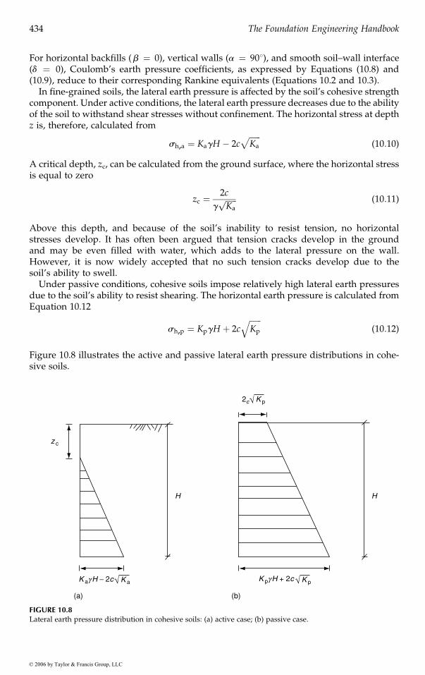
In fine-grained soils, the lateral earth pressure is affected by the soil’s cohesive strengthcomponent. Under active conditions, the lateral earth pressure decreases due to the abilityof the soil to withstand shear stresses without confinement. The horizontal stress at depthz is, therefore, calculated from
sh,a ¼ KagH � 2cffiffiffiffiffiffiKa
p(10:10)
A critical depth, zc, can be calculated from the ground surface, where the horizontal stressis equal to zero
zc ¼2c
gffiffiffiffiffiffiKa
p (10:11)
Above this depth, and because of the soil’s inability to resist tension, no horizontalstresses develop. It has often been argued that tension cracks develop in the groundand may be even filled with water, which adds to the lateral pressure on the wall.However, it is now widely accepted that no such tension cracks develop due to thesoil’s ability to swell.
Under passive conditions, cohesive soils impose relatively high lateral earth pressuresdue to the soil’s ability to resist shearing. The horizontal earth pressure is calculated fromEquation 10.12
sh,p ¼ KpgH þ 2cffiffiffiffiffiffiKp
q(10:12)
Figure 10.8 illustrates the active and passive lateral earth pressure distributions in cohe-sive soils.
z c
2c
H H
K agH − 2c√ K a
√ K p
(a) (b)
K pgH + 2c √ K p
FIGURE 10.8Lateral earth pressure distribution in cohesive soils: (a) active case; (b) passive case.
Gunaratne / The Foundation Engineering Handbook 1159_C010 Final Proof page 434 22.11.2005 2:56am
434 The Foundation Engineering Handbook
© 2006 by Taylor & Francis Group, LLC

Example 10.1
Calculate the lateral earth pressure against the retaining wall shown in Figure 10.9 underboth active and passive conditions. The backfill consists of coarse sand with a unit weightof 17.5 kN/m3 and an internal friction angle of 308. The angle of interface friction, d,between the wall and the soil is 158.
SolutionSince the wall–soil interface is rough, Coulomb’s theory must be used since Rankine’ssolution is limited to smooth interfaces. We first calculate Coulomb’s coefficients of activeand passive earth pressure from Equations (10.8) and (10.9), respectively:
KA ¼sin (90� � 30�)= sin 90�
ffiffiffiffiffiffiffiffiffiffiffiffiffiffiffiffiffiffiffiffiffiffiffiffiffiffiffiffiffiffisin (90� þ 15�)
pþ
ffiffiffiffiffiffiffiffiffiffiffiffiffiffiffiffiffiffiffiffiffiffiffiffiffiffiffiffiffiffiffiffiffiffiffiffiffiffiffiffiffiffiffiffiffiffiffiffiffiffiffiffiffiffiffiffiffiffiffiffisin (30� þ 15�) sin (30� � 10�)
sin (90� � 10�)
s
0BBBB@
1CCCCA
2
¼ 0:343
KP ¼sin (90� þ 30�)= sin 90�
ffiffiffiffiffiffiffiffiffiffiffiffiffiffiffiffiffiffiffiffiffiffiffiffiffiffiffiffiffiffisin (90� � 15�)
p�
ffiffiffiffiffiffiffiffiffiffiffiffiffiffiffiffiffiffiffiffiffiffiffiffiffiffiffiffiffiffiffiffiffiffiffiffiffiffiffiffiffiffiffiffiffiffiffiffiffiffiffiffiffiffiffiffiffiffiffiffisin (30� þ 15�) sin (30� þ 10�)
sin (90� � 10�)
s
0BBBB@
1CCCCA
2
¼ 8:14
A
Sand
B
Pa
Passive
997 kPa
Pp
Active
42 kPa
b = 10�
g = 17.5 kN/m3
j = 30�
d = 15�
15�
15�
FIGURE 10.9Illustration for Example 10.1.
Gunaratne / The Foundation Engineering Handbook 1159_C010 Final Proof page 435 22.11.2005 2:56am
Retaining Walls: Analysis and Design 435
© 2006 by Taylor & Francis Group, LLC

Next, we calculate the vertical effective stress at points A and B. Here, since there is nowater table behind the wall, the total and effective stresses are equal. At the top of thewall, since there is no surcharge, the vertical stress is equal to zero. At point B, the verticalstress is calculated by multiplying the unit weight of the soil by the height of the wall
svð ÞA ¼ 0
svð ÞB ¼ gH ¼ 17:5� 7 ¼ 122:5 kPa
Multiplying the vertical stress by the corresponding coefficient of lateral earth pressure,we obtain the active and passive lateral earth pressure
sh,active
� �A¼ sh,passive
� �A¼ 0
sh,active
� �B¼ svð ÞA � KA ¼ 122:5� 0:343 ¼ 42 kPa
sh,passive
� �B¼ svð ÞA � KP ¼ 122:5� 8:14 ¼ 997 kPa
Because of the friction that develops between the wall and the soil, the active and passivepressures act at downward and upward 158 angles, respectively, measured from hori-zontal. The pressure increases linearly with depth. Accordingly, the resultant force acts ata distance of H/ 3 from the bottom of the wall. The resultant force per unit width of thewall can be calculated by computing the area of the triangular pressure distribution
PA ¼1
2sh,active
� �BH ¼ 0:5� 42� 7 ¼ 147 kN=m
PP ¼1
2sh,passive
� �BH ¼ 0:5� 997� 7 ¼ 3490 kN=m
10.3 Basic Design Principles
In resisting lateral earth pressure, a variety of mechanisms may act independently or incombination to provide the stability of the earth retaining structure. Gravity and canti-
structure counteracting the external forces acting on the wall surface (Figure 10.10a).Tie-back anchorage, developing along the grouted portion of the anchor, provides thebulk of the resistance in walls and sheet piles, as illustrated in Figure 10.10(b). MSE wallsare monolithic internally stable reinforced earth structures that derive their strength fromthe tensile forces mobilized along the reinforcement strips (Figure 10.10c). It is importantto stress that for MSE walls, the role of the facing units is mainly aesthetic, with secondaryfunctions such as erosion control.
Most design methods are based on limiting equilibrium considerations, with little orno consideration given to the deformation of the system. Most commonly used is theallowable stress design (ASD) method, in which the forces acting on or within the systemare analyzed at equilibrium. A global factor of safety, FS, is typically calculated based onthe generic equation:
FS ¼ Stabilizing forces or moments
Applied forces or moments(10:13)
Gunaratne / The Foundation Engineering Handbook 1159_C010 Final Proof page 436 22.11.2005 2:56am
436 The Foundation Engineering Handbook
© 2006 by Taylor & Francis Group, LLC
lever walls (Figure 10.10) rely on their own weight for stability, with the self-weight of the
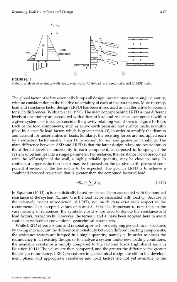
The global factor of safety essentially lumps all design uncertainties into a single quantity,with no consideration to the relative uncertainty of each of the parameters. More recently,load and resistance factor design (LRFD) has been introduced as an alternative to accountfor such differences (Withiam et al., 1998). The main concept behind LRFD is that differentlevels of uncertainty are associated with different load and resistance components withina given system. For instance, consider the gravity retaining wall shown in Figure 10.10(a).Each of the load components, such as active earth pressure and surface loads, is multi-plied by a specific load factor, which is greater than 1.0, in order to amplify the distressand account for uncertainties in loads. Similarly, the resisting forces are multiplied eachby a reduction factor smaller than 1.0 to account for soil and geometric variability. Themain difference between ASD and LRFD is that the latter design takes into considerationthe different levels of uncertainty in each component, as opposed to lumping all thesystem uncertainties into a single parameter. For instance, the resistance factor associatedwith the self-weight of the wall, a highly reliable quantity, may be close to unity. Incontrast, a larger reduction factor may be imposed on the passive earth pressure com-ponent if erosion of the toe soil is to be expected. The goal in LRFD is to achieve acombined factored resistance that is greater than the combined factored load:
hRn �X
liQi (10:14)
In Equation (10.14), h is a statistically based resistance factor associated with the nominalresistance of the system, Rn, and li is the load factor associated with load Qi. Because ofthe relatively recent introduction of LRFD, not much data exist with respect to therecommended or accepted values of h and li. It is also important to note that, in thevast majority of references, the symbols w and gi are used to denote the resistance andload factors, respectively. However, the terms h and li have been adopted here to avoidconfusion with other conventional geotechnical parameters.
While LRFD offers a sound and rational approach for designing geotechnical structuresby taking into account the difference in reliability between different loading components,the resistance factors are lumped in a single quantity, namely h. In order to assess theredundancy in an existing design, or to analyze a system under new loading conditions,the available resistance is simply compared to the factored loads (right-hand term inEquation 10.14). The values are then compared, and the greater the difference the greaterthe design redundancy. LRFD procedures in geotechnical design are still in the develop-ment phase, and appropriate resistance and load factors are not yet available to the
(a) (b) (c)
W
Earthpressure
F1
T1
T2
T3
F2
FIGURE 10.10Stability analysis of retaining walls: (a) gravity walls, (b) tie-back anchored walls, and (c) MSE walls.
Gunaratne / The Foundation Engineering Handbook 1159_C010 Final Proof page 437 22.11.2005 2:56am
Retaining Walls: Analysis and Design 437
© 2006 by Taylor & Francis Group, LLC

geotechnical engineer. ASD is still widely accepted among the geotechnical community,and is the specified method in most current design codes. Therefore, in this chapter, wewill focus the attention on the ASD method in solving example problems.
10.3.1 Effect of Water Table
In many instances, the soil behind an earth retaining structure is submerged. Examplesinclude seawalls, sheet-pile walls in dewatering projects, and offshore structures. Anotherreason for saturation of backfill material is poor drainage, which leads to an undesirablebuildup of water pressure behind the retaining wall. Drainage failure often results insubsequent failure and collapse of the earth retaining structure.
In cases where the design considers the presence of a water table, the lateral earthpressure is calculated from the effective soil stress. Oddly enough, this leads to a reductionin effective horizontal earth pressure since the effective stresses are lower than their totalcounterpart. However, the total stresses on the wall increase due to the presence of thehydrostatic water pressure. In other words, while the effective horizontal stress decreases,the total horizontal stress increases. The next example illustrates this concept.
Example 10.2Due to clogging of the drainage system, the water table has built up to a depth of 4 mbelow the ground surface behind the retaining wall shown in Figure 10.11. The soil abovethe water table is partially saturated and has a unit weight of 17 kN/m3. Below the watertable, the soil is saturated and has a unit weight of 19 kN/m3. Calculate the total andeffective vertical and horizontal stresses at point A under active conditions.
SolutionFirst, we calculate the total and effective vertical stress at point A
Total vertical stress ¼ svð ÞA¼ 17� 4þ 19� 2 ¼ 106 kPa
Pore water pressure ¼ uA ¼ gwzw ¼ 9:8� 2 ¼ 19:6 kPa
Effective vertical stress ¼ s0v� �
A¼ 106� 19:6 ¼ 86:4 kPa
Next, we calculate the coefficient of lateral earth pressure using Equation (10.2)
Ka ¼1� sin 33�
1þ sin 33�¼ 0:295
4 m
GWT
g = 17 kN/m3
j = 338
gsat = 19 kN/m32 mA
FIGURE 10.11Illustration for Example 10.2.
Gunaratne / The Foundation Engineering Handbook 1159_C010 Final Proof page 438 22.11.2005 2:56am
438 The Foundation Engineering Handbook
© 2006 by Taylor & Francis Group, LLC

We then calculate the effective horizontal stress using Equation (10.1)
Effective horizontal stress ¼ s0h� �
A¼ Ka s0v
� �A¼ 0:295� 86:4 ¼ 25:5 kPa
The total horizontal stress is calculated by adding the pore water pressure to the effectivehorizontal stress
Total horizontal stress ¼ shð ÞA¼ s0h� �
Aþ uA ¼ 25:5þ 19:6 ¼ 45:1 kPa
It is important to note that the total horizontal stress cannot be correctly calculated bymultiplying the total vertical stress by the coefficient of lateral earth pressure
shð ÞA 6¼ Ka svð ÞA
Such calculation will result in significant underestimation of the horizontal stresses actingon a retaining structure under active conditions.
10.3.2 Effect of Compaction on Nonyielding Walls
In the case of rigid (nonyielding) walls, at-rest conditions are considered in the structuraldesign. In addition, locked-in passive earth pressures can develop near the top of the wallif heavy compaction equipment is used. The passive condition, caused by a line load Pfrom the roller, develops from the ground surface up to a depth of zp and remainsconstant to a depth of zr where:
zp ¼
ffiffiffiffiffiffiffiffiffiffiffiffiffiffiffiffi2PKaK0
pg
s, zr ¼
ffiffiffiffiffiffiffiffiffiffiffiffiffiffiffiffiffi2P
pgKaK0
s
Below a depth of zr, at-rest earth pressure conditions prevail. In the case of flexible walls,such conditions are not believed to occur due to wall displacement. Instead, activeconditions are assumed. In addition, light compaction equipment is typically used tocompact the backfill behind most retaining walls in order to reduce the lateral earthpressures. As a result, the additional earth pressure due to compaction may not need tobe considered, depending on the construction method.
10.4 Gravity Walls
In the past, gravity and cantilever walls constituted the vast majority of earth retainingstructures. However, in recent years, these structures have given way to MSE walls,which are more economical, easier to construct, and better performing. A small numberof projects, however, still rely on gravity walls and their closely related support system ofmodular block walls. Traditionally, gravity walls are cast in place of plain or reinforcedconcrete structures that rely on their own weight for stability. They may be constructed in
Modular block walls, on the other hand, are constructed by stacking rows of interlock-ing blocks and compacting the soil in successive layers. Masonry or cinder blocks can alsobe used in conjunction with mortar binding to form limited height walls, typically no
Gunaratne / The Foundation Engineering Handbook 1159_C010 Final Proof page 439 22.11.2005 2:56am
Retaining Walls: Analysis and Design 439
© 2006 by Taylor & Francis Group, LLC
a wide range of geometries, some of which are illustrated in Figure 10.12.

taller than 2 m. Interlocking blocks are available commercially in a wide variety of shapesand materials, some of which are proprietary. They provide a greater level of stabilitythan masonry walls and are sometimes manufactured so that the resulting facing isbattered (see Figure 10.13).
In designing gravity walls, external stability, which is the equilibrium of all externalforces, is more critical than the internal structural stability of the wall. This is mostly dueto the massive nature of the structure, which usually results in conservative designs forinternal stability. In analyzing or designing for external stability, all the forces acting onthe structure are considered. These forces include lateral earth pressures, the self-weightof the structure, and the reaction from the foundation soil. The stability of the wall is thenevaluated by considering the relevant forces for each potential failure mechanism.
The four potential failure mechanisms typically considered in design or analysis are
FIGURE 10.12Typical geometries of gravity retaining walls.
FIGURE 10.13Modular block wall with battered facing.
Gunaratne / The Foundation Engineering Handbook 1159_C010 Final Proof page 440 22.11.2005 2:56am
440 The Foundation Engineering Handbook
© 2006 by Taylor & Francis Group, LLC
shown in Figure 10.14 and are summarized next:

1. Sliding resistance. The net horizontal forces must be such that the wall is pre-vented from sliding along its foundation. The factor of safety against sliding iscalculated from:
FSsliding ¼P
Resisting forcesPSliding forces
(10:15)
The minimum acceptable limit for FSsliding is 1.5. The most significant sliding forcecomponent usually comes from the lateral earth pressure acting on the active(backfill) side of the wall. Such force may be intensified by the presence of verticalor horizontal loads on the backfill surface. In the unlikely event where a watertable is present within the backfill, the water pressure may reduce the lateral earthpressure due to the reduction in effective stresses, but greater lateral forces aregenerated on the wall from the hydrostatic pressure of the water itself. The maincomponent resisting the sliding is the friction along the wall base. Due to thepotential for erosion, the passive earth pressure in front of the toe of the wall isconservatively ignored in design. If such passive earth pressure is included, thenthe minimum acceptable limit for FSsliding increases to 2.0.
Sliding
Bearing capacity
Global instability
Overturning
FIGURE 10.14Potential failure modes due to external instability of gravity walls.
Gunaratne / The Foundation Engineering Handbook 1159_C010 Final Proof page 441 22.11.2005 2:56am
Retaining Walls: Analysis and Design 441
© 2006 by Taylor & Francis Group, LLC

2. Overturning resistance. The righting moments must be greater than the over-turning moments to prevent rotation of the wall around its toe. The rightingmoments result mainly from the self-weight of the structure, whereas the mainsource of overturning moments is the active earth pressure. The factor of safetyagainst overturning is calculated from:
FSoverturning ¼P
Righting momentsPOverturning moments
(10:16)
The factor of safety against overturning must be equal to or greater than 1.5.
3. Bearing capacity. The bearing capacity of the foundation soil must be largeenough to resist the stresses acting along the base of the structure. The factorof safety against bearing capacity failure, FSBC, is calculated from:
FSBC ¼qult
qmax(10:17)
where qult is the ultimate bearing capacity of the foundation soil, and qmax is themaximum contact pressure at the interface between the wall structure and thefoundation soil. The minimum acceptable value for FSBC is 3.0. In addition to‘‘traditional’’ bearing capacity considerations, the movement of the wall due toexcessive settlement of the underlying soil must also be limited. The componentsof the foundation settlement include immediate, consolidation, and creep settle-ment, depending on soil type.
4. Global stability. Overall stability of the wall system within the context of slopestability must also be assessed to ensure that no failure occurs either in thebackfill or the native soil. As such, a separate analysis for slope stability must beperformed on the zone in the vicinity of the wall using conventional limitequilibrium slope stability methods.
When considering the active and passive earth pressures on either side of the wall forsliding and overturning calculations, caution must be exercised. The wall movementneeded to fully mobilize an active condition on one side of the wall is much smaller thanthat needed to mobilize the passive pressure on the other side. For sands, a horizontaldeformation of approximately 0.0025 to 0.0075 of the wall height is required to reach theminimum earth pressure on the active side, with lower displacement corresponding to stiff(dense) sand. The horizontal displacement needed to develop the full passive resistance isapproximately 10 times that amount, which raises the issue of displacement compatibility.Even though the soil on the passive side is typically looser due to the lack of overburdenconfinement, a fully passive condition rarely develops within typical acceptable displace-ment ranges in retaining walls. This lack of displacement compatibility may even be moresignificant if the rotation mechanism of the wall is considered. It is, therefore, advised toneglect the passive earth pressure in wall stability calculations.
If a design proves to be inadequate, remedial action must be taken to increase the
additional soil may be compacted in front of the wall toe, but provisions are needed toensure that such soil does not erode with time. Another solution is the inclusion of a
Gunaratne / The Foundation Engineering Handbook 1159_C010 Final Proof page 442 22.11.2005 2:56am
442 The Foundation Engineering Handbook
© 2006 by Taylor & Francis Group, LLC
corresponding factor of safety (see Figure 10.15). In the case of potential sliding failure,
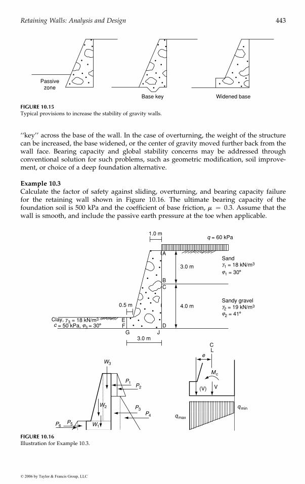
‘‘key’’ across the base of the wall. In the case of overturning, the weight of the structurecan be increased, the base widened, or the center of gravity moved further back from thewall face. Bearing capacity and global stability concerns may be addressed throughconventional solution for such problems, such as geometric modification, soil improve-ment, or choice of a deep foundation alternative.
Example 10.3Calculate the factor of safety against sliding, overturning, and bearing capacity failurefor the retaining wall shown in Figure 10.16. The ultimate bearing capacity of thefoundation soil is 500 kPa and the coefficient of base friction, m ¼ 0.3. Assume that thewall is smooth, and include the passive earth pressure at the toe when applicable.
Passivezone
Base key Widened base
FIGURE 10.15Typical provisions to increase the stability of gravity walls.
1.0 mq = 60 kPa
3.0 m
Sand
Sandy gravel
g1 = 18 kN/m3
g2 = 19 kN/m3
Clay, g 3 = 18 kN/m3
c = 50 kPa, j3 = 308
j1 = 308
j2 = 418
4.0 m
3.0 m
0.5 m
A
BC
DJG
W3
Mc
V(V)
qmax
qmin
e
CL
W2
W1
P1P2
P3
P6P5
P4
EF
FIGURE 10.16Illustration for Example 10.3.
Gunaratne / The Foundation Engineering Handbook 1159_C010 Final Proof page 443 22.11.2005 2:56am
Retaining Walls: Analysis and Design 443
© 2006 by Taylor & Francis Group, LLC

Solution
the right and left side of the wall, respectively. Accordingly, we calculate the coefficientsof active earth pressure for the sand and the sandy gravel layers, and passive earthpressure for the clay layer:
Ka1 ¼1� sin 30�
1þ sin 30�¼ 0:333
Ka2 ¼1� sin 41�
1þ sin 41�¼ 0:208
Kp3 ¼1þ sin 10�
1� sin 10�¼ 1:42
We then calculate the vertical and horizontal stresses at points A through F. Within eachsoil layer, the horizontal stresses increase linearly since the soil is uniform and homoge-neous. It is also important to note that the horizontal stress at point B is different frompoint C since there is an ‘‘abrupt’’ change in the coefficient of lateral earth pressure at thatlocation. It is also noted that the passive pressure at points E and F is calculated fromEquation (10.12) due to the presence of cohesion in the clay.
The next step is to calculate the resultant vertical and horizontal forces by subdividingthe lateral earth pressure diagram and the wall cross section into rectangles and triangles.The earth pressure forces are calculating from the area of the diagram, while the weightsof the concrete wall are calculated by multiplying the area by the unit weight of concrete(23.5 kN/m3). It is also prudent at this stage to compute the moment arm associated witheach force (measured from the wall toe F) in anticipation of the overturning stabilitycalculations.
Point s0v (kPa) K s0h (kPa)
A 60 0.333 60 � 0.333 ¼ 20B 60 þ 18 � 3 ¼ 114 0.333 114 � 0.333 ¼ 38C 114 0.208 114 � 0.208 ¼ 23.7D 114 þ 19 � 4 ¼ 190 0.208 190 � 0.208 ¼ 39.5E 0 1.42 2 � 50 � (1.42)0.5 ¼ 119.2F 16 � 1 ¼ 16 1.42 119 þ 16 � 1.42 ¼ 141.7
Force Magnitude (kN/m) Moment Arm (m)
P1 20 � 3 ¼ 60 4 þ 3/2 ¼ 5.5P2
12 (38 � 20) � 3 ¼ 27 4 þ 3/3 ¼ 5
P3 23.7 � 4 ¼ 94.8 4/2 ¼ 2P4
12 (39.5 � 23.7) � 4 ¼ 31.6 4/3 ¼ 1.33
P5 119.2 � 1 ¼ 119.2 1/2 ¼ 0.5P6
12 (141.7 � 119.2) � 1 ¼ 11.25 1/3 ¼ 0.33
W1 3 � 1 � 23.5 ¼ 70.5 3/2 ¼ 1.5W2
12 � 1.5 � 6 � 23.5 ¼ 105.8 0.5 þ 1.5 � 2/3 ¼ 1.5
W3 1 � 7 � 23.5 ¼ 164.5 2.5Fb SWim ¼ (70.5 þ 105.8 þ 164.5) � 0.3 ¼ 102.2 0
Gunaratne / The Foundation Engineering Handbook 1159_C010 Final Proof page 444 22.11.2005 2:56am
444 The Foundation Engineering Handbook
© 2006 by Taylor & Francis Group, LLC
Based on the conditions shown in Figure 10.16, active and passive earth pressures act on

The factor of safety against sliding is calculated from Equation (10.15):
FSsliding ¼P5 þ P6 þ Fb
P1 þ P2 þ P3 þ P4¼ 232:7
213:4¼ 1:09
The factor of safety against overturning is calculated from Equation (10.16):
FSoverturning ¼119:2�0:5þ11:25�0:33þ70:5�1:5þ105:8�1:5þ164:5�2:5
60�5:5þ27�5þ94:8�2þ31:6�1:33¼ 739
697¼ 1:06
In calculating the resisting moments, the passive earth pressure at the toe of the wallwas included in this example. This should only be done in cases where it is guaranteedthat such soil will not erode. Otherwise, the moments resulting from the passive earthpressure at the toe of the wall should be ignored.
In order to calculate the factor of safety against bearing capacity failure, it is necessaryto determine the maximum and minimum base contact pressures. Due to the eccentricitygenerated by the moment, the maximum pressure will typically occur at the toe of thewall (point G) while the minimum will occur at the heel (point J). The total vertical force,V ¼ SW, and the moment, Mc, about the center of the base are equivalent to a verticalforce V acting at an eccentric distance e from the center of the base. An easy method forcalculating e relies on the righting and overturning moments about the toe, which areavailable from the FSoverturning calculations:
e ¼ b
2�MR �MO
V
where b is the width of the base, MR and MO are the righting and overturning moments,respectively, and V ¼ SW is the summation of the vertical forces. Therefore,
e ¼ 3
2� 739� 697
70:5þ 105:8þ 164:5¼ 1:38 m
The maximum and minimum pressures are then calculated from basic mechanics ofmaterials concepts:
qmax ¼V
b1þ 6
e
b
� �, qmin ¼
V
b1� 6
e
b
� �
As such,
qmax ¼340:8
31þ 6� 1:38
3
� �¼ 427:1 kPa
The factor of safety against bearing capacity failure is calculated from Equation (10.17):
FSBC ¼qult
qmax¼ 500
427:1¼ 1:2
It is evident in this problem that the wall is marginally safe, since the factors of safetyagainst sliding, overturning, and bearing capacity are slightly above 1.0. However, thesevalues are much lower than the recommended values of 2.0, 1.5, and 3.0, respectively.Therefore, the design modifications should be introduced to increase the factors of safetyto their minimum acceptable limits.
Gunaratne / The Foundation Engineering Handbook 1159_C010 Final Proof page 445 22.11.2005 2:56am
Retaining Walls: Analysis and Design 445
© 2006 by Taylor & Francis Group, LLC

10.5 Cantilever Walls
Like gravity walls, cantilever retaining walls have also become largely obsolete, but areconstructed in cases where MSE walls are not feasible. They also rely on their self-weightto resist sliding and overturning, but derive part of their stability from the weight of thebackfill above the heel of the wall. Cantilever walls are made of reinforced concrete, andcome in different geometries. They are often easier to erect than gravity wall, since theycan be prefabricated in sections and transported directly to the site. Figure 10.17 showsisometric views of simple cantilever walls and counterfort walls.
In addition to the external stability, cantilever walls must also satisfy internal structural
withstand the shear stresses and bending moments resulting from the lateral earthpressure as well as the difference in pressure between the top and bottom faces of thebase. To this end, steel reinforcement is placed as shown in the figure. The size anddensity of the reinforcement are decided by the structural engineer, based on the struc-tural design of the cross section. Counterforts are used to reduced shear forces andbending moments at the critical section where higher walls are needed.
When considering the external stability of the wall, the backfill section above the canti-lever wall heel is assumed to be part of the wall, with Rankine or Coulomb conditions
tion is largely accurate, provided that the width of the heel is larger than [H tan(458� w/2)],which is typically true except for tall walls. The weight of the soil block above the heel isthen added to the weight of the reinforced concrete wall in all stability calculations. Allprocedures for stability checks are identical to those described for gravity walls.
Example 10.4
b, required to ensure stability of the wall against overturning. In addition, determine theangle, u, of the potential active shear plane with respect to horizontal.
(a) (b)
FIGURE 10.17General view of (a) cantilever retaining wall and (b) counterfort wall.
Gunaratne / The Foundation Engineering Handbook 1159_C010 Final Proof page 446 22.11.2005 2:56am
446 The Foundation Engineering Handbook
© 2006 by Taylor & Francis Group, LLC
stability requirements. As shown in Figure 10.18, the wall section should be able to
acting along the vertical line originating at the heel (line AB in Figure 10.19). This assump-
For the cantilever retaining wall shown in Figure 10.20, calculate the width of the heel,

SolutionIn order to facilitate the calculation process, we divide the cantilever wall into sections. Wethen calculate the weight per unit width (Wi) and moment arm (xi) for each block:
W1 ¼ 23:5� 0:5� 0:7 ¼ 8:23 kN (per meter)
W2 ¼ 23:5� 5� 0:5 ¼ 58:75 kN
W3 ¼ 23:5� 0:5� b ¼ 11:75b kN
W4 ¼ (17� 2:5þ 19� 2)b ¼ 80:5b kN
Pressuredistribution Shear
stresses
Bendingmoments
FIGURE 10.18Schematic of shear and bending moment diagrams of cantilever wall.
Rigidsoil
block
Activeearth
pressure
B
A
FIGURE 10.19Rigid soil block assumption for design of cantilever retaining wall.
Gunaratne / The Foundation Engineering Handbook 1159_C010 Final Proof page 447 22.11.2005 2:56am
Retaining Walls: Analysis and Design 447
© 2006 by Taylor & Francis Group, LLC

x1 ¼ 0:35 m
x2 ¼ 0:95 m
x3 ¼ 1:20þ b=2
x4 ¼ 1:20þ b=2
We then calculate the active earth pressure and the water pressure on the wall. For lateralearth pressure calculations, we use Ka ¼ tan2(45 � 35/2) ¼ 0.271
s0h1 ¼ 17� 2:5� 0:271 ¼ 11:52 kPa
s0h2 ¼ ð17� 2:5þ f19� 9:8g � 2:5Þ � 0:271 ¼ 17:75 kPa
u ¼ 9:8� 2:5 ¼ 24:5 kPa
The corresponding forces (per meter), P1 to P4, together with their moment arms, y1 to y4,are calculated as follows:
0.5 m
2.5 m
0.5 m
GWT
Sand
Sand
g = 17 kN/m3
gsat = 19 kN/m3
j = 358
j = 358
s �h1
s �h2
0.7 m
W2W4
P1
P2
P3
u
P4W3
W1
Sand 0.5 m
bq
FIGURE 10.20Illustration for Example 10.4.
Gunaratne / The Foundation Engineering Handbook 1159_C010 Final Proof page 448 22.11.2005 2:56am
448 The Foundation Engineering Handbook
© 2006 by Taylor & Francis Group, LLC
P1 ¼ 0:5� 11:52� 2:5 ¼ 14:4 kN
P2 ¼ 17:75� 2:5 ¼ 44:38 kN
P3 ¼ 0:5� (17:75� 11:52)� 2:5 ¼ 7:79 kN
P4 ¼ 0:5� 24:5� 2:5 ¼ 30:63 kN
y1 ¼ 2:5þ 2:5=3 ¼ 3:33 m
y2 ¼ 2:5=2 ¼ 1:25 m
y3 ¼ y4 ¼ 2:5=3 ¼ 0:83 m
The factor of safety against overturning is calculated from
FSoverturning ¼P4
i¼1 WixiP4i¼1 Piyi
¼ 8:23� 0:35þ 58:75� 0:95þ 11:75b� (1:2þ b=2)þ 80:5b� (1:2þ b=2)
14:4� 3:33þ 44:38� 1:25þ 7:79� 0:83þ 30:63� 0:83
In order to ensure stability, the factor of safety must be at least equal to 1.5. Accordingly,we solve the equation above for b and obtain:
b ¼ 1 m
The angle, u, that the potential active failure surface makes with respect to horizontal issimply equal to 45 þ w/2 ¼ 45 þ 35/2 ¼ 62.5.
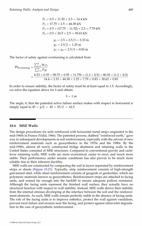
10.6 MSE Walls
The design procedures for soils reinforced with horizontal metal strips originated in themid-1960s in France (Vidal, 1966). The patented process, dubbed ‘‘reinforced earth,’’ gaveway to subsequent developments in soil reinforcement, especially with the advent of newreinforcement materials such as geosynthetics in the 1970s and the 1980s. By themid-1990s, almost all newly constructed bridge abutment and retaining walls in theUnited States consisted of MSE structures. Compared to conventional gravity and canti-lever retaining walls, MSE walls are more economical, easier to erect, and much morestable. Their performance under seismic conditions has also proven to be much morereliable due to their inherent ductility.
MSE walls are constructed by compacting the soil in layers separated by reinforcement
galvanized steel, while sheet reinforcement consists of geogrids or geotextiles, which arepolymeric materials known as geosynthetics. Reinforcement strips are attached to facingunits, and extend far enough into the backfill to ensure adequate pullout resistance.Although the facing units represent the finished wall surface, they actually have nostructural function with respect to wall stability. Instead, MSE walls derive their stabilityfrom the internal stresses developing at the interface between the soil and the reinforce-ment elements. As such, MSE walls remain perfectly stable in the absence of facing units.The role of the facing units is to improve esthetics, protect the wall against vandalism,prevent local failure and erosion near the facing, and protect against ultraviolet degrada-tion in the case of geosynthetic reinforcement.
Gunaratne / The Foundation Engineering Handbook 1159_C010 Final Proof page 449 22.11.2005 2:56am
Retaining Walls: Analysis and Design 449
© 2006 by Taylor & Francis Group, LLC
strips or sheets (Figure 10.21). Typically, strip reinforcement consists of high-strength

Originally, all external stability requirements (sliding, overturning, bearing capacity,and global stability) needed to be checked for MSE wall design. However, it has beenfound that, due to their monolithic nature, MSE walls are not prone to overturning. Inaddition, MSE walls must be designed to ensure internal stability, which includes checksagainst yielding and pullout of reinforcement. The design must also ensure adequateconnection strength between reinforcement and facing in the case of timber or concretepanels.
10.6.1 Internal Stability Analysis and Design
The internal stability requirements for MSE walls dictate the extent of the reinforcementelements into the backfill, as well as their vertical and (if strips are used) horizontal spacing.
assumed vertical spacing, the vertical stresses are calculated at each reinforcement depth (z).The corresponding horizontal stress, sh,z, is then computed accordingly, assuming activeearth pressure conditions. The horizontal earth pressure at depth z is calculated from:
sh,z ¼ Kasv,z (10:18)
In the absence of any surcharge loading, the vertical stress is equal to the unit weight ofthe soil times the depth. Additional stresses resulting from surcharges at the surface maybe calculated from a variety of methods such as elastic solutions and charts whenapplicable. The maximum tensile force in the reinforcement layer is calculated by multi-plying the horizontal stress by the cross sectional ‘‘area of influence’’ of the reinforcementelement. In the case of reinforcement strips, the area of influence is equal to sv � sh, wheresv and sh are the vertical and horizontal spacing between the reinforcement strips,respectively. In the case of geogrid and geotextile reinforcement, a unit width of thereinforcement is considered in lieu of the horizontal spacing, sh. In this case, the calcula-tion output is a force per unit length.
The factor of safety against yielding of the reinforcement is then calculated for eachlayer by dividing the yield strength of the reinforcement material by the maximum tensilestrength:
FSyielding ¼Fmax
sh,z � sv � sh� 1:5 (10:19)
FIGURE 10.21General view of MSE wall.
Gunaratne / The Foundation Engineering Handbook 1159_C010 Final Proof page 450 22.11.2005 2:56am
450 The Foundation Engineering Handbook
© 2006 by Taylor & Francis Group, LLC
Figure 10.22 represents a generic cross section of an MSE wall. Based on the existing or

where Fmax is the maximum design tensile resistance of the reinforcement element. In thecase of galvanized steel, the yield strength may be used. However, in the case of geosyn-thetic reinforcement, the yield strength must be multiplied by a number of reductionfactors to account for environmental conditions. As such, the maximum design strengthof geosynthetic reinforcement is calculated from:
Fmax ¼ Fyield � RFCR � RFID � RFCD � RFBD (10:20)
where RFCR, RFID, RFCD, and RFBD are reduction factors for creep deformation, installa-tion damage, chemical degradation, and biological degradation, respectively. These val-ues depend on the properties of the geosynthetic as well as the environmental conditionsduring operation and can vary within a very significant range. It is not uncommon forthese factors to amount to an overall reduction factor of 10 or 20.
The second component of internal stability is the resistance to pullout, which dictates theextent of the reinforcement into the backfill. For design purposes, a potential Rankine-typefailure wedge (u ¼ 45þ w/2) is considered to originate at the toe of the wall (Figure 10.22).The length of reinforcement within the Rankine wedge, LR, is calculated from
LR ¼ (H � z) tan (45� w=2) (10:21)
Experimental evidence has shown that a Rankine wedge may not be representative of theactual potential failure surface, so more sophisticated design procedures may considermore realistic surfaces, such as curved or bilinear failure wedges. Since the failure wedgeis assumed to be rigid, no internal deformations develop, and the length of reinforcementwithin this zone (LR) does not contribute to resisting pullout. Instead, the effective lengthof reinforcement (Le) is measured from the back end of the Rankine wedge. The factor ofsafety against pullout resistance is calculated by dividing the available pullout resistanceby the maximum tensile force in the reinforcement for each reinforcement layer:
FSpullout ¼2� w� sv,z � tan wi � Le
sh,z � sv � sh� 1:5 (10:22)
LR Le
Sv
H
Backfill
Native soil
Rankin
e
Z
45 + f /2
FIGURE 10.22Cross section of MSE wall.
Gunaratne / The Foundation Engineering Handbook 1159_C010 Final Proof page 451 22.11.2005 2:56am
Retaining Walls: Analysis and Design 451
© 2006 by Taylor & Francis Group, LLC

where w is the width of the reinforcement element and wi is the interface friction anglebetween the soil and the reinforcement. It is noted that a multiplier of 2 is included in thenumerator to account for frictional stresses developing on both top and bottom faces ofthe embedded reinforcement. The total length, LT, of the reinforcement for each layer isthen calculated by adding the Rankine length, LR, to the effective length, Le.
For reinforcement elements distributed at uniform spacing, it is inevitable that designcalculations will result in different required yield strength and length for each layer ofreinforcement. However, from a constructability perspective, it is imperative to specify aconstant set of values, corresponding to the most critical layer. As a result, the finisheddesign ends up being overly conservative and extremely redundant in safety. In largeprojects where tall MSE walls are constructed, and when strict quality control measuresare implemented in the field, it is possible to specify multiple sets of parameters overcertain heights of the wall. For instance, it is not uncommon to use tighter verticalreinforcement spacing within the bottom half of a wall, where tensile forces are highest.
10.6.2 Reinforced Earth Walls
Reinforced earth walls are earth retaining structures that consist of steel strips connectedto uniquely shaped concrete or metal facing panels. The most common facing design isthe prefabricated concrete panel system shown in Figure 10.23, although other designshave also been used. Reinforcement elements consist of galvanized steel strips, approxi-mately 0.1 m wide and 5 mm thick, with a patterned surface to enhance frictionalinteraction with the soil. Four strips are connected to each facing unit. Among the mostcritical issues concerning the response of these walls is corrosion of the steel strips,especially in marine environments. In such cases, the use of geosynthetic reinforcementmay be warranted.
FIGURE 10.23Reinforced earth wall facing panel system.
Gunaratne / The Foundation Engineering Handbook 1159_C010 Final Proof page 452 22.11.2005 2:56am
452 The Foundation Engineering Handbook
© 2006 by Taylor & Francis Group, LLC

Design of reinforced earth walls and similar MSE systems starts by determining thereinforcement vertical and horizontal spacing. These values are typically predeterminedfrom the geometry of the prefabricated concrete facing panels. Typical values of verticaland horizontal spacing are 0.75 and 0.5 m, respectively. A suitable reinforcement materialis then chosen based on Equation (10.19), and the reinforcement length is determined. Inaddition, the connection at the facing must be able to sustain the maximum tensile forcesin the reinforcement, although, in reality, the forces at the connection are much smaller.
Example 10.5An MSE wall is reinforced with galvanized steel strips, spaced at 0.75 m vertically and0.5 m horizontally. The strips are 0.10 m wide, and the yield strength of the galvanizedsteel is 240 MPa. The wall height is 9 m, and the backfill consists of select granularmaterial with w ¼ 358 and g ¼ 18 kN/m3. The soil–steel interface friction angle is 258.A surcharge of 200 kPa is applied at the top of the wall. Calculate the minimum requiredthickness of the steel strips and the total embedment length.
SolutionSince the wall height is 9 m, and the vertical spacing between the reinforcement layers is0.75 m, the total number of reinforcement layers is 12, with the first layer embedded at0.375 m from the top. Typically, it is advisable to perform all calculations in a tabulated(spreadsheet) format, with each row corresponding to a soil layer. In this particularexample, because a uniform surcharge is applied at the top, the maximum horizontalstresses will develop at the bottom layer, where z ¼ 8.625 m
sh,z ¼ Ka(qþ gz) ¼ 1� sin 35�
1þ sin 35�� (200þ 18� 8:625) ¼ 96:3 kPa
From Equation (10.19) and assuming FSyielding ¼ 1.5, we determine Fmax
Fmax ¼ 1:5� 96:3� 0:75� 0:5 ¼ 54:2 kN
The thickness of the steel strip is determined from the width and yield strength of the steelstrips:
t ¼ Fmax
syield � w¼ 54:2
240,000� 0:1¼ 2:3� 10�3 m ¼ 2:3 mm
A minimum of 2 mm is typically added as a sacrificial thickness since corrosion is all butcertain. Therefore, the total thickness is equal to 4.3 mm, which is rounded to the nearestpractical thickness of 5 mm.
The effective length of reinforcement, Le, is calculated from Equation (10.22), by assum-ing a factor of safety of 1.5. Since the ratio between sh,z and sv,z is equal to Ka, the value ofLe is independent of depth, and is calculated from
Le ¼1:5� Ka � sv � sh
2� w� tan wi
¼ 1:5� 0:271� 0:75� 0:5
2� 0:1� tan 25�¼ 1:63 m
The maximum value of LR (Rankine length) will occur at the top layer, where z ¼ 0.375.From Equation (10.21), LR ¼ (9 � 0.375) tan(45 � 35/2) ¼ 4.49 m. The total length, LT, isequal to
LT ¼ Le þ LR ¼ 1:63þ 4:49 ¼ 6:12 m
The value of LT is rounded to the nearest practical length of 6.25 m.
Gunaratne / The Foundation Engineering Handbook 1159_C010 Final Proof page 453 22.11.2005 2:56am
Retaining Walls: Analysis and Design 453
© 2006 by Taylor & Francis Group, LLC

10.6.3 Geogrid-Reinforced Walls
With the increased availability of high-strength geogrid materials in the 1990s, geogrid-reinforced walls were introduced as an alternative to metallic strip reinforcement. Theyprovide increased interface area (since the coverage area can be continuous), betterinterlocking with the backfill (due to the geometry of the openings), resistance to corro-sive environments, and lower cost. The most common type of geogrids used in earthreinforcement is the uniaxial type, owing to its high strength and stiffness in the maindirection. Facing panel units may be connected to the geogrid using a steel bar inter-woven into the grid (known as a Bodkin connector) or, more recently, through specialplastic clamps that tie into a geogrid section embedded in the concrete panel.
Among the concerns associated with the use of geogrids in heavily loaded walls (such asbridge abutments) are the time-dependent stress relaxation (creep deformation), installa-tion damage, and chemical degradation. It is, therefore, crucial to determine the designstrength of the geogrid considering the various reduction factors described in Equation(10.20). In addition, it is extremely important to ensure that the geogrid is fully stretchedduring installation and compaction of the subsequent soil layer. Otherwise, significantdeformation is needed before tensile stresses and interface friction is mobilized. A closelyrelated problem that has been identified is the difficulty in keeping the facing elementsplumb during installation, especially when close tolerance is needed in tall walls.
Design and construction procedures for geogrid-reinforced walls are almost identicalto reinforced earth walls. One distinct exception is that the strength of the geogrid isexpressed in terms of force per unit length, and the associated horizontal spacing, sh, istaken as the unit length in all calculations. Another difference is that, because of theeffective interlocking of the soil particles within the geogrid openings, the interfacefriction angle is usually equal to the internal friction angle of the soil.
10.6.4 Geotextile-Reinforced Walls
Unlike metallic and geogrid reinforcement, typical geotextile-reinforced wall designs donot require facing elements. Instead, the geotextile layer is wrapped around the com-pacted soil at the front to form the facing (Figure 10.24). The finished wall must becovered with shotcrete, bitumen, or Gunite to prevent ultraviolet radiation from reachingand damaging the geotextile. Such walls are usually constructed as temporary structures,or where aesthetics are not of prime importance. However, it is possible to cover the wallwith a permanent ‘‘faux finish’’ that blends with the surrounding environment.
Geotextile
reinforcement
FIGURE 10.24Geotextile-reinforced wall with wrapped-around facing.
Gunaratne / The Foundation Engineering Handbook 1159_C010 Final Proof page 454 22.11.2005 2:56am
454 The Foundation Engineering Handbook
© 2006 by Taylor & Francis Group, LLC

The design procedures for geotextile-reinforced walls are also identical to those de-scribed earlier for steel and geogrid reinforcement. The interface friction angle betweenthe soil and the geotextile sheet is typically equal to (1/2)w to (2/3)w. In addition, theoverlap length, Lo must be determined from the following equation:
Lo ¼sv � sh,z
2sv,z � tan wi
� FSoverlap (10:23)
The minimum acceptable overlap length is 1 m.
10.7 Sheet-Pile and Tie-Back Anchored Walls
Sheet-pile walls provide temporary or permanent support when excavations are to becarried out. They consist of steel, concrete, and sometimes timber sections, typicallydriven in the ground using percussion, vibration, or jetting. More recently,fiber-reinforced polymers (FRPs) have been used successfully in a number of projectswhere the sheet piles are driven to shallow depths. FRPs have the advantage of resisting awide range of chemically aggressive environments. Typical cross sections of sheet piles(in plan view) are shown in Figure 10.25.
Once driven in the ground, excavation proceeds on one side, with the sheet pile provid-ing the necessary earth support. For shallow depths (less than 6 m), cantilever-type sheet
the excavation level can deliver the moment required to resist the lateral earth pressure onthe active side. For larger excavation depths, it becomes necessary to supplementthe embedment resistance with a tie-rod anchor at a shallow depth. Such tie-rod anchorsare often installed by excavating and re-compacting the soil. If multiple rows of anchors arerequired, a tie-back anchored retaining wall is constructed by driving the anchors andgrouting them in place.
10.7.1 Cantilever Sheet Piles
A conceptual representation of the lateral earth pressure acting on a cantilever sheet pile
surface to the depth of excavation. Below the excavation depth, passive conditions areassumed to act on Side B of the sheet pile, while active conditions persist on Side A, up topoint O, where a reversal of conditions occurs. Point O can be viewed roughly as the pointof rotation of the sheet pile in the ground. Such rotation is necessary in order to achievestatic equilibrium of the system. Below point O, active conditions develop on Side B whilepassive earth pressures are present on Side A.
(a) (b)
FIGURE 10.25Typical cross sections of sheet-pile materials: (a) steel, and (b) concrete.
Gunaratne / The Foundation Engineering Handbook 1159_C010 Final Proof page 455 22.11.2005 2:56am
Retaining Walls: Analysis and Design 455
© 2006 by Taylor & Francis Group, LLC
piles are adequate (Figure 10.26). In this case, the embedment depth of the sheet pile below
is shown in Figure 10.27. Only active pressure is present on Side A, from the ground

Cantilever sheet-pile design typically involves the determination of the embedmentdepth, D, given other geometric constraints of the problem as well as soil properties.Therefore, the first step is to calculate the magnitude of the horizontal stresses sA, sB, andsC. The value of sA is readily calculated as the active earth pressure acting at depth H. Themagnitudes of sO and sB must be calculated as a function of the embedment depth, D,and the depth to the rotation point, D1, both of which are unknown. The value of sO iscalculated assuming passive conditions on Side B and active conditions on Side A.Similarly, sB is calculated with passive earth pressure on Side A and active earth pressureon Side B. Two equilibrium conditions are to be satisfied: the sum of the horizontal forcesand the sum of the moments in the system must be equal to zero. By solving bothequilibrium equations, the two unknowns, D and D1, can be determined.
As force and moment calculations become complex, it is often convenient to determinethe value of sC, which is the hypothetical lateral earth pressure at depth D that corres-ponds to passive earth pressure on Side B and active earth pressure on Side A. As will beshown in the Example 10.6, the forces and their line of action are found easier through thisprocedure.
Tie-rodanchor
(a) (b) (c)
Ld
FIGURE 10.26Typical sheet-pile support mechanisms: (a) cantilever sheet pile, (b) tie-rod anchored sheet pile, and (c) tie-backanchored wall.
H
Side B Side A
Bottom of excavation
D
C
O
D1
sO
sB sC
sA
FIGURE 10.27Conceptual representation of lateral earth pressure on a cantilever sheet-pile wall.
Gunaratne / The Foundation Engineering Handbook 1159_C010 Final Proof page 456 22.11.2005 2:56am
456 The Foundation Engineering Handbook
© 2006 by Taylor & Francis Group, LLC

Example 10.6
For the sheet-pile wall shown in Figure 10.28, determine the minimum depth of exc-avation required to achieve equilibrium.
SolutionFor the clay layer, Ka (from Equation 10.2) is equal to 0.406. The depth horizontal stress atpoint A is determined from Equation (10.10) and the critical depth zc from Equation(10.11):
sA ¼ 0:406� 16� 5� 2� 20�ffiffiffiffiffiffiffiffiffiffiffi0:406p
¼ 7:0 kPa
zc ¼2� 20
16ffiffiffiffiffiffiffiffiffiffiffi0:406p ¼ 3:92 m
The coefficients of active and passive lateral earth pressure, Ka and Kp, for the sand layerare equal to 0.333 and 3.0, respectively. The horizontal stress at the top of the sandlayer (point B) is thus equal to
sB ¼ 0:333� 16� 5 ¼ 26:7 kPa
The horizontal stress at point F is equal to the difference between passive pressure to theleft side of the sheet pile and active pressure to the right:
sF ¼ 3� 17�D� 0:333� (16� 5þ 17�D) ¼ 45:34D� 26:7 kPa
Similarly, the lateral earth pressure at G is equal to the difference between passiveconditions on the right side of the sheet pile and active conditions on the left:
sG ¼ 3� (16� 5þ 17�D)� 0:333� 17�D ¼ 45:34Dþ 240 kPa
It is possible to determine the lateral forces in the sheet piles by calculating the areas oftriangles RNA, BRC, CEM, and MGQ. However, such calculations become cumbersomedue to the fact that depths D and D1 are unknown. Instead, it is possible to consider anequivalent set of forces, P1 to P4, such that the net earth pressure is the same:
1. P1 is equal to the area of triangle RNA.
2. P2 is equal to the area of rectangle RBJQ.
H = 5 m
D
D1P3 P4
P1
zo
P2
F
E
C
N
Q J G
M
AB
Sand
Clayg = 16 kN/m3
g = 17 kN/m3
j = 25�
j = 30�
c = 20 kPa
FIGURE 10.28Illustration for Example 10.6.
Gunaratne / The Foundation Engineering Handbook 1159_C010 Final Proof page 457 22.11.2005 2:56am
Retaining Walls: Analysis and Design 457
© 2006 by Taylor & Francis Group, LLC

3. P3 is equal to the area of triangle BJF.
4. P4 is equal to the area of triangle EFG.
We then calculate the forces, Pi, and their corresponding moment arms, yi, from point R
P1 ¼ (1=2)(5:0� 3:92)(7:0) ¼ 3:78 kN
P2 ¼ (D)(26:7) ¼ 26:7D
P3 ¼ �(1=2)(D)(26:7þ 45:34D� 26:7) ¼ �22:67D2
P4 ¼ (1=2)(D1)(45:34D� 26:7þ 45:34Dþ 240) ¼ (D1)(45:34Dþ 106:7)
y1 ¼ 13ð5:0� 3:92Þ ¼ 0:36 m
y2 ¼ �12 D
y3 ¼ �23D
y4 ¼ �ðD� 13D1Þ
The next step is to satisfy the equations of equilibrium, in terms of horizontal forces andmoments about point R
X4
i¼1
Pi ¼ 0
3:78þ 26:7D� 22:67D2 þD1(45:34Dþ 106:7) ¼ 0
X4
i¼1
Piyi ¼ 0
(3:78)(0:36)� (26:7D)(12D)þ (22:67D)(2
3D)� (D1)(45:34Dþ 106:7)(D� 13D1) ¼ 0
Solving the two equations above simultaneously, we obtain:
D ¼ 2:1 m (and D1 ¼ 0:2 m)
The actual embedment depth is calculated by multiplying the theoretical depth by a factorof safety of 1.2. Therefore, the actual embedment depth is equal to 1.2D ¼ 2.5 m.
10.7.2 Anchored Sheet Piles
For large excavation depths the inclusion of an anchor tie rod is necessary in order toreduce the moment on the sheet-pile wall. Otherwise, unreasonably large cross sectionsmay be needed in order to resist the moment. Anchored sheet piles may be analyzedusing either the free-earth support or the fixed-earth support method. Under free-earth
and rotate in the ground. Only active earth pressures develop on the tie-back side, whilepassive pressures act on the other side. No stress reversal of rotation points exist down theembedded depth of the sheet pile. In contrast, the tip of fixed-earth support sheet piles isassumed to be restricted from rotation. Stress reversal occurs down the embedded depth,and the sheet pile is analyzed as a statically indeterminate structure.
To design free-earth support sheet piles, typically the depth of the anchor tie rod needsto be known. Equilibrium conditions are checked in terms of horizontal forces andmoments, and the force in the tie rod as well as the depth of embedment are calculatedaccordingly. Alternatively, the maximum allowable force in the tie rod may be given, with
Gunaratne / The Foundation Engineering Handbook 1159_C010 Final Proof page 458 22.11.2005 2:56am
458 The Foundation Engineering Handbook
© 2006 by Taylor & Francis Group, LLC
support conditions, the tip of the sheet pile (Figure 10.29) is assumed to be free to displace

the depth of the tie rod and the embedment depth of the sheet pile as unknowns. It isusually convenient to sum the system moments about the connection of the tie rod withthe sheet pile to eliminate the tensile force in the tie rod from the equation.
The necessary anchor resistance in the tie rod is supplied through an anchor plate ordeadman located at the far end of the tie rod (Figure 10.29a). In order to ensure stability, theanchor plate must be located outside the active wedge behind the sheet pile, which isdelineated by line AB from the tip. In addition, this active wedge must not interfere with thepassive wedge through which the tension in the tie rod is mobilized, which is bounded bythe ground surface and line BC. Therefore, the length of the tie rod, Lt is calculated from
Lt ¼ (H þD) tan (45� � w=2)þDt tan (45� þ w=2) (10:24)
Example 10.7For the sheet-pile wall shown in Figure 10.29(a), determine the depth of embedment, D,and the force in the tie rod. The soil on both sides of the sheet pile is well-graded sand,
A
No rotation
H1
H
Pa
(a)
(b)
T
D t
45−j /2
45+j /2
B
Anchorplate
Anchorplate
D Pp
O
FIGURE 10.29Conceptual representation of lateral earth pressure on tie-rod anchored sheet-pile walls: (a) free-earth support,and (b) fixed-earth support.
Gunaratne / The Foundation Engineering Handbook 1159_C010 Final Proof page 459 22.11.2005 2:56am
Retaining Walls: Analysis and Design 459
© 2006 by Taylor & Francis Group, LLC

with a unit weight g ¼ 19 kN/m3 and an internal friction angle of 348. The tie rods arespaced at 3 m horizontally, and are embedded at a depth H1 ¼ 1 m. The height of theexcavation H ¼ 15 m.
SolutionThe active force, Pa, on the right side is calculated from
Pa ¼ (1=2)Kag(H þD) ¼ (1=2)� 0:283� 19� (15þD) ¼ 40:328þ 2:689D
The passive force, Pp, on the right side is calculated from
Pp ¼ (1=2)KpgD ¼ (1=2)� 3:537� 19�D ¼ 33:60D
The sum of the moments about point O is
(40:328þ 2:689D)(23f15þDg � 1)� (33:60D)(15þ 2
3D) ¼ 0
Solving for D, we obtain:
D ¼ 0.77 mThe tension in the tie rods per meter width of the sheet-pile wall is then calculated fromthe equilibrium of the horizontal forces:
T (per meter) ¼ (40:328þ 2:689� 0:77)� (33:60� 0:77) ¼ 16:53 kN=m
The force in each tie rod is calculated by multiplying the result by the horizontal spacing:
T ¼ 3� 16:53 ¼ 50 kN
The theoretical depth, D, is multiplied by a safety factor of 1.2, thereby giving a totalembedment depth of 0.92 m, which is rounded to 1.0 m.
10.7.2.1 Redundancy in Design
It is important to note that, when the theoretical depth of embedment of the sheet pile ismultiplied by a safety factor of 1.2, the resulting depth does not satisfy equilibriumconditions. In reality, when the depth of embedment is extended, full passive conditionsdo not develop. Therefore, if an analysis of the stability of an existing sheet pile is carriedout, it would be incorrect to consider the earth pressure diagrams used in design. Instead,it is common practice to redesign the sheet-pile structure and then check the redundancyby calculating the factor of safety as
FS ¼ Actual embedment depth
Theoretical embedment depth(10:25)
10.7.3 Braced Excavations
Excavations in urban environments are constrained by the lack of adjacent space forinstalling tie rods or ground anchors. Where cantilever sheet piles are impractical, itbecomes imperative to provide support to the sheet piles through internal bracing and
to ensure that the bracing system is stiff enough to prevent or minimize adjacent ground
Gunaratne / The Foundation Engineering Handbook 1159_C010 Final Proof page 460 22.11.2005 2:56am
460 The Foundation Engineering Handbook
© 2006 by Taylor & Francis Group, LLC
struts. Examples of typical braced excavations are shown in Figure 10.30. It is important

movement, and strong enough to resist the earth pressure associated with such restricteddeformations. Construction is usually initiated by driving the sheet piles or lateralsupport system, then excavating gradually from the ground level down. Rows of bracingor lateral support are installed as the excavation progresses down.
The earth pressure developing in the case of braced excavations is different from thetheoretical linear increase with depth described earlier for conventional retaining walls. Inbraced excavations, the lateral earth pressure is dictated by the sequence of excavation,soil type, stiffness of the wall and struts, and movement allowed prior to installing thestruts. Although accurate determination of the distribution of earth pressure in bracedcuts is almost impossible, Terzaghi et al. (1996) provide approximate methods based onactual observations for use in strut design (Figure 10.31). In the case of sands, theenvelope of the apparent earth pressure is constant and equal to 0.65KagH, where H isthe depth of the excavation. In the case of soft/medium clays, and stiff fissured clays, thediagrams shown in Figure 10.31(b) and (c) are used, respectively. It is imperative, how-ever, to monitor the development of forces in the struts and deformations along the depthof the braced cut during construction. Forces in the struts and deformations must becontinuously adjusted to comply with design specifications.
10.7.4 Tie-Back Anchored Walls
In cases where adequate land adjacent to an excavated site is available, the use of tie-backanchors is preferred over braced cuts. Tie-back anchors do not interfere with the spaceavailable for construction equipment mobilization in the excavation, and can be used as
FIGURE 10.30Examples of braced excavations.
Forcesfrom
struts
Forcesfrom
struts
Forcesfrom
strutsH
(a) (b) (c)
0.65KagH (0.2 to 0.4) g KagH
1/4H 1/4H
1/4H
3/4H
3/4H
FIGURE 10.31Approximate earth pressure diagrams for use in designing braced excavations: (a) sand, (b) soft to medium clay,and (c) stiff fissured clay.
Gunaratne / The Foundation Engineering Handbook 1159_C010 Final Proof page 461 22.11.2005 2:56am
Retaining Walls: Analysis and Design 461
© 2006 by Taylor & Francis Group, LLC
permanent earth retaining systems. Construction proceeds by first driving soldier pilesinto the ground. Soldier piles are individual sections, typically steel I-beams that aredriven in the ground at close spacing (1 or 2 m). Excavation is then carried out in stages, 1to 2 m deep at a time, with timber lagging placed in between the soldier piles to preventsoil collapse. Tie-back anchors are subsequently installed at different levels, and locked in
sists of directionally drilling in the soil, typically at a 158 angle, then sliding a PVC ormetal perforated casing into the hole. A steel anchor cable or rod is then inserted into thecasing, and grout is injected to fill the casing around the cable and permeate through thecasing perforations into the surrounding soil. The grouted zone must be fully locatedoutside the active wedge (458 þ w/2) measured from the bottom of the excavation. Thetension at each level can be adjusted by tightening or loosening a lock nut at theconnection between the tie-back anchor and the wall. Walls very large in height can beconstructed using this technique. An alternative procedure for building tie-back anchoredwalls involves the construction of a concrete wall by slurry replacement, followed by asimilar excavation and tie-back anchoring procedure, as described above.
When determining the maximum pullout resistance of a tie-back anchor, it is importantto determine the soil type, and whether the structure is temporary or permanent. Forpermanent walls in clays, the use of effective stress analysis concepts is essential incalculating the long-term pullout capacity. On the other hand, total stress analysis (un-drained conditions) may be adopted for short-term evaluation of tie-back anchor capacity.For tie-back anchors in sand, the maximum capacity, Tult, is calculated from
Tult ¼ pdpgL tan w (10:26)
where d is the diameter of the grouted bulb, pg is the earth pressure on the grout, L is thegrouted length, and w is the friction angle of the soil. The value of pg may be taken as K0s0vfor shallow depths, where arching is not expected in the soil. Alternatively, based on fieldmeasurements of typical grouted anchors, the value of pdpg may be taken to be equal to500 kN/m for coarse granular materials, and 150 kN/m for fine sands. For undrainedanalysis in clays, Tult, is calculated from
Tult ¼ 0:3pdLSu (10:27)
where Su is the undrained shear strength (undrained cohesion) of the clay.The factor of safety for pullout resistance is typically taken to be 3 or 4 for long-term
analysis and 2 for short-term analysis. Tie-back anchors are tested in the field, postcon-struction, at 1.5 times their desired capacity. In case of failure, the anchor is regrouted andretested.
10.8 Soil Nail Systems
Soil nailing is a technique for stabilizing steep slopes and vertical cuts. The techniquerelies on driving soil nails, which are steel rods 25 to 50 mm in diameter, into a vertical or
may be installed through drilling and grouting. Conceptually, the method differs fromtie-back anchored walls in that no prior driving or installation of an earth retaining wall(sheet pile, soldier piles, or slurry wall) is conducted. Instead, the exposed soil surface is
Gunaratne / The Foundation Engineering Handbook 1159_C010 Final Proof page 462 22.11.2005 2:56am
462 The Foundation Engineering Handbook
© 2006 by Taylor & Francis Group, LLC
place to support the retaining structure (Figure 10.31c). The installation procedure con-
steep cut at a 158 angle as excavation proceeds (Figure 10.32). Alternatively, the soil nails

kept from caving in by installing a wire mesh on which the soil nails are connected throughface plates. The technique works best in cohesive soils, since significant unraveling mayoccur in sandy soils. The wire mesh is then covered with shotcrete, and excavation isproceeded to the next level. Soil nail walls are typically used as temporary earth retainingsystems, although they have been used successfully as permanent structures.
When analyzing soil nail systems, global stability is considered. Conventional methodsfor slope stability analysis are used, with the tension in the soil nails contributing to thestability of the slope. Typically, the method of slices is chosen, and the forces actingon each slice, including the tensile resistance of the soil nail are included. The globalstability of the reinforced soil mass is then assessed, and a factor of safety is calculated.The length of the soil nails is determined accordingly, so as to satisfy equilibrium of theslope or vertical cut.
10.9 Drainage Considerations
Proper drainage of backfill materials is a crucial component of retaining wall design.In general, cohesive backfills are highly undesirable because of their poor drainage, loss ofstrength and increase in density upon wetting, and high coefficient of active earthpressure. This is particularly important in the case of MSE walls, where only selectbackfill material may be used. Acceptable soil types for such purpose are SW(well-graded sand), GW (well-graded gravel), and SP (poorly graded sand). The vastmajority of current design codes prohibit the use of cohesive materials as backfill in MSEwalls.
In addition, proper drainage provisions must be included in the design. This entails the
Shotcretefacing
FIGURE 10.32Construction of soil-nailed wall.
Gunaratne / The Foundation Engineering Handbook 1159_C010 Final Proof page 463 22.11.2005 2:56am
Retaining Walls: Analysis and Design 463
© 2006 by Taylor & Francis Group, LLC
inclusion of drains and filters in the cross section, such as those shown in Figure 10.33.

While graded sand constituted the majority of filters and drains in the past, geosynthetics(geotextiles, geonets, and geocomposites) are used in almost all projects today. In order toselect the proper filter material, the acceptable apparent opening size (O95) of the geosyn-thetic must be first determined. Current guidelines require that O95 be smaller than2.5D85, where D85 is the grain size corresponding to 85 percentile on the grain sizedistribution of the soil. Geonets selected for drainage must have a maximum flow ratethat is greater than the anticipated flow rate in the structure.
10.10 Deformation Analysis
Recently, the recognition of the importance of limiting deformation levels in retainingwalls has led to the emergence of deformation-based design approaches. Because all suchmethods require accurate estimation of the stress–strain behavior of soils, by itself adifficult task, deformation-based design is limited to large projects where, for instance,soil parameters can be determined accurately from extensive laboratory tests. Finiteelement analyses can then be performed to determine the anticipated levels of deforma-tion under a given set of boundary conditions, and the wall design is modified accord-ingly to result in acceptable deformations.
In projects where deformation is critical, such as bridge approaches and abutments,deformations are typically monitored during construction to ensure they remain withinthe acceptable range. In situations where tie-back anchored sheet-pile walls are con-structed, the tension within the tie-backs may be adjusted at the connection between thefacing and the tie-backs to prevent excessive deformations during construction. Levels ofdeformation required to achieve active and passive conditions during construction, for
Weep-holes
Edgedrain
Collectionpipe
Drain
Filte
r
FIGURE 10.33Drainage provisions in cantilever retaining wall.
Gunaratne / The Foundation Engineering Handbook 1159_C010 Final Proof page 464 22.11.2005 2:56am
464 The Foundation Engineering Handbook
© 2006 by Taylor & Francis Group, LLC
different soil types, are given in Table 10.1.

10.11 Performance under Seismic Loads
In seismically active areas, it is essential to consider the additional seismic forces acting onthe earth retaining structure during design. For gravity and cantilever walls, the proced-ure most widely used in practice is the Mononobe–Okabe method, as modified by Seedand Whitman (1970). The method considers the stability of Coulomb-type wedge in amanner similar to that used in static design (Figure 10.34). However, an equivalentseismic load is assumed to act at the center of gravity of the wedge, with horizontal andvertical magnitudes equal to the mass of the wedge times the horizontal and verticalaccelerations, respectively. The force resulting from the combination of static earth pres-sure and seismic loading is assumed to act at a height of 0.6H from the bottom of the wall.The active earth pressure resultant force on the wall, PAE, is calculated from:
PAE ¼ (1=2)KAEg(1� kv)H2 (10:28)
KAE ¼cos2 (w� c� uv)
cos c cos2 uv cos (cþ uv þ d) 1þffiffiffiffiffiffiffiffiffiffiffiffiffiffiffiffiffiffiffiffiffiffiffiffiffiffiffiffiffiffiffiffiffiffiffiffiffiffiffiffiffiffiffisin (w þ d) sin (w � c � b)
cos (b � uv) cos (c þ uv þ d)
q� �2(10:29)
c ¼ kh
1� kv(10:30)
where kv is the vertical acceleration in gs, c is the seismic inertia angle calculatedfrom Equation (10.30), uv is the inclination of the wall with respect to vertical, b is theslope angle of the ground surface, and d is the soil–wall interface friction angle.
H
d
q
j
b
W
R
W kv
W kh
PAE
FIGURE 10.34Mononobe–Okabe stability wedge under seismic loading.
Gunaratne / The Foundation Engineering Handbook 1159_C010 Final Proof page 465 22.11.2005 2:56am
Retaining Walls: Analysis and Design 465
© 2006 by Taylor & Francis Group, LLC

Similarly, the force on the wall under passive earth pressure conditions is calculatedfrom:
PPE ¼ (1=2)KPEg(1� kv)H2 (10:31)
KPE ¼cos2 (w� cþ uv)
cos c cos2 uv cos (c� uv þ d) 1�
ffiffiffiffiffiffiffiffiffiffiffiffiffiffiffiffiffiffiffiffiffiffiffiffiffiffiffiffiffiffiffiffiffiffiffiffiffiffiffiffiffiffiffiffiffiffiffiffiffiffiffiffiffiffiffiffiffisin (wþ d) sin (w� cþ b)
cos (b� uv) cos (c� uv þ d)
s !2(10:32)
Field observations of postearthquake conditions of MSE walls indicate minimal damageto the structure. This is partly due to the high level of redundancy in design, but is mostlyattributed to the ductility of the structure.
10.12 Additional Examples
Example 10.8The concrete retaining wall shown in Figure 10.35 retains a granular backfill. The angle offriction between the backfill and concrete is 128. Determine the resultant force on the walldue to the earth pressure, its direction, and the line of action.Based on the figure, 4 m ¼ 5 cm
Hence, the top width ¼ 0.72 m and the bottom width ¼ 2 m
a ¼ 180� � tan [14=(2� 0:72)] ¼ 180� � 72� ¼ 108�
b ¼ 0
d ¼ 12�
N ¼ 30�
Granular backfillAngle of friction = 20�Unit weight =17.0 kN/m3
4 m
1.33 m
12�
FIGURE 10.35Illustration for Example 10.8.
Gunaratne / The Foundation Engineering Handbook 1159_C010 Final Proof page 466 22.11.2005 2:56am
466 The Foundation Engineering Handbook
© 2006 by Taylor & Francis Group, LLC

Using Coulomb’s active earth pressure coefficient (Equation 10.8)
KA ¼sin (a� w)= sin a
ffiffiffiffiffiffiffiffiffiffiffiffiffiffiffiffiffiffiffiffiffiffisin (aþ d)
pþ
ffiffiffiffiffiffiffiffiffiffiffiffiffiffiffiffiffiffiffiffiffiffiffiffiffiffiffiffiffiffiffiffiffiffiffiffiffiffiffiffiffiffiffiffiffisin (wþ d) sin (w� b)
sin (a� b)
s
0BBBB@
1CCCCA
2
¼ 0:455
The pressure diagram can be determined by the following equation:
sh;a ¼ KagH � 2cffiffiffiffiffiffiKa
p
¼ 0:455(17)z ¼ 7:735z (see the plot in figure)(10:10)
where PA is the area of the pressure diagram equal to
Z4
0
[7:735z]dz ¼ 61:88 kN=m
The line of action and direction are indicated in the figure.
Example 10.9
granular backfill
(i) Plot the lateral earth pressure exerted on the sheet pile.
(ii) Plot the Mohr circles for points on the sheet pile at depths of 1 m and 6 m fromthe top.
(iii) Accurately indicate the failure surface
g ¼ Gs þ Seð Þgw
1þ e¼ 11:8 kN=m3
where Gs ¼ 2.65, Se ¼ 0, and e ¼ 1.2
gs ¼2:65þ 1� 1:2ð Þ
1þ 1:29:8 ¼ 17:15 kN=m3
For sandy soil
Ka ¼ cos acos a�
ffiffiffiffiffiffiffiffiffiffiffiffiffiffiffiffiffiffiffiffiffiffiffiffiffiffiffiffifficos2 a� cos2p
f
cos aþffiffiffiffiffiffiffiffiffiffiffiffiffiffiffiffiffiffiffiffiffiffiffiffiffiffiffiffifficos2 a� cos2p
f¼ 0:5312; where a ¼ 10�; f ¼ 20�
or
Ka ¼sin (a� f)= sin a
ffiffiffiffiffiffiffiffiffiffiffiffiffiffiffiffiffiffiffiffiffiffisin (aþ d)
pþ
ffiffiffiffiffiffiffiffiffiffiffiffiffiffiffiffiffiffiffiffiffiffiffiffiffiffiffiffiffiffiffiffiffiffiffiffiffiffiffiffiffiffiffiffiffisin (aþ d) sin (f� b)
sin (a� b)
s
266664
377775
2
¼ 0:569 � 0:57
(10:8)
Gunaratne / The Foundation Engineering Handbook 1159_C010 Final Proof page 467 22.11.2005 2:56am
Retaining Walls: Analysis and Design 467
© 2006 by Taylor & Francis Group, LLC
The steel sheet pile shown in Figure 10.36(a) is embedded in clayey ground and retains a
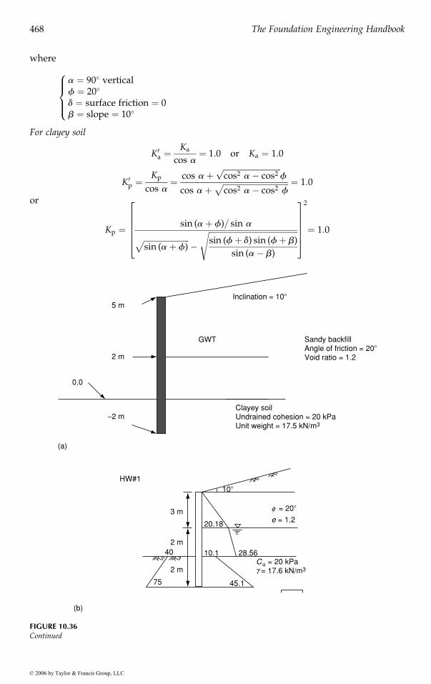
where
a ¼ 90� verticalf ¼ 20�
d ¼ surface friction ¼ 0b ¼ slope ¼ 10�
8>><>>:
For clayey soil
K0a ¼Ka
cos a¼ 1:0 or Ka ¼ 1:0
K0p ¼Kp
cos a¼ cos aþ
ffiffiffiffiffiffiffiffiffiffiffiffiffiffiffiffiffiffiffiffiffiffiffiffiffiffiffiffifficos2 a� cos2p
f
cos aþffiffiffiffiffiffiffiffiffiffiffiffiffiffiffiffiffiffiffiffiffiffiffiffiffiffiffiffiffiffiffiffifficos2 a� cos2 f
p ¼ 1:0
or
Kp ¼sin (aþ f)= sin a
ffiffiffiffiffiffiffiffiffiffiffiffiffiffiffiffiffiffiffiffiffiffiffisin (aþ f)
p�
ffiffiffiffiffiffiffiffiffiffiffiffiffiffiffiffiffiffiffiffiffiffiffiffiffiffiffiffiffiffiffiffiffiffiffiffiffiffiffiffiffiffiffiffiffisin (fþ d) sin (fþ b)
sin (a� b)
s
266664
377775
2
¼ 1:0
Inclination = 10�
Clayey soilUndrained cohesion = 20 kPaUnit weight = 17.5 kN/m3
Sandy backfillAngle of friction = 20�Void ratio = 1.2
GWT
0.0
(a)
2 m
5 m
−2 m
10�
20.18
f = 20�
e = 1.23 m
HW#1
2 m40
2 m
75
(b)
10.1
45.1
28.56Cu = 20 kPag = 17.6 kN/m3
FIGURE 10.36Continued
Gunaratne / The Foundation Engineering Handbook 1159_C010 Final Proof page 468 22.11.2005 2:56am
468 The Foundation Engineering Handbook
© 2006 by Taylor & Francis Group, LLC

s �v = 0
s �v = 11.8 � 3 = 35.4s �ha = 35.4 � 0.57 = 20.18 kPa
s �v = 35.4 + (17.15 − 9.8) � 2 = 50.1,
s �v = 50.1 + (17.5) � 2 = 85.1,
s �ha = ka s v − 2c ka = 50.1 − 2 � 20 = 10.1 kPa
s �v = 85.1 − 2 � 20 = 45.1 kPa
swater (kPa)
s ha (kPa)s hp (kPa)
s �ha = 50.1 � 0.57 = 28.56 kPa,sN = 9.8 � 2 = 4,
s �v = 17.5 � 2 = 35
s �h,w = 0
σ4 = 0
3 m
2 m
2 m
(c)
(d)
√
s �hp = 1 � 35 + 2 � 20 1 = 757 kPa√
s hp = kp s v + 2c Kp = 40 kPa √
20.18
10.140
75
28.56
45.1
19.6
6.7 17.5 27.6 67.657.5
11.8
(e)
FIGURE 10.36(a) Illustration for Example 10.9. (b) Earth pressure distribution on the sheet pile. (c) Earth pressure computa-tions for Example 10.9. (d) Earth and water pressure distributions for Example 10.9. (e) Mohr circle plots forExample 10.9.
Gunaratne / The Foundation Engineering Handbook 1159_C010 Final Proof page 469 22.11.2005 2:56am
Retaining Walls: Analysis and Design 469
© 2006 by Taylor & Francis Group, LLC

(ii) Stresses at depths of 1 m and 6 m from the top:
Active side at 1 m
sv ¼ 11:8� 1 ¼ 11:8 kPa
sha ¼ 0:57� 11:8 ¼ 6:7 kPa
Active side at 6 m
sv ¼ 11:8� (17:15� 9:8)� 2þ 17:15� 1 ¼ 67:6 kPa
sha ¼ 1� 67:6� 2� 20ffiffiffi1p¼ 27:6 kPa
Passive side at 6 m
sv ¼ 17:5� 1 ¼ 17:5 kPa
shp ¼ 1� 17:5þ 2� 20ffiffiffi1p¼ 57:5 kPa
Example 10.10Estimate the passive pressure on the wall shown in Figure 10.37(a) by selecting a trialfailure surface shown. The backfill supports a highway pavement of width 4.5 m, whichimposes a distributed load of 40 kPa.Horizontal, b ¼ 08
Length ¼ 5
sin 45�¼ 7:07 m
Soil area ¼ (1/2)(6.5)(5) ¼ 16.25 m2
Clayey soilUndrained strength = 20 kPaUnit weight = 17.0 kN/m3
Wall friction angle = 10�5.0 m
2 m 3.5 m 3.0 m
3.5 m
(a)
FIGURE 10.37Continued
Gunaratne / The Foundation Engineering Handbook 1159_C010 Final Proof page 470 22.11.2005 2:56am
470 The Foundation Engineering Handbook
© 2006 by Taylor & Francis Group, LLC

W1 ¼ 16.25 � 17 ¼ 276.25 kN/mW2 ¼ (40)(3) ¼ 120 kN/mW ¼ W1 þ W2 ¼ 396.25 kN/mC ¼ Su(length) ¼ 20(7.07) ¼ 141.4 kN/m
For passive lateral force, the wall will be pushed inside, moves right.By measuring according to scale,
� Pp ¼ 420 kN=m
Example 10.11
sliding. Assume that the stem and the base are of width 0.5 m.
3.5 m
1.5 m
5 m
W1
Pp
W2
2.0 m
3.0 m
C
R
Length
f = 0
d = 40 kPa
z = 10�
16.7�45�
90
45� = Pa = 73.3�
(b)
6.7�
83.3�
Pp
51.7�
W = 396.25 kN/m
C = 141.4 kN/m
135�
90�
By measuring according to scale Pp = 420 kN/m
R
(c)
FIGURE 10.37(a) Illustration for Example 10.10. (b) Free-body diagram for Example 10.10. (c) Force polygon for Example 10.10.
Gunaratne / The Foundation Engineering Handbook 1159_C010 Final Proof page 471 22.11.2005 2:56am
Retaining Walls: Analysis and Design 471
© 2006 by Taylor & Francis Group, LLC
Investigate the stability of the concrete retaining wall shown in Figure 10.38(a) against

(a)
Surcharge = 30 kPa
GWT,Elev. 2 m
Backfill ofclayey soilUndrainedstrength = 20 kPaDry unit weight= 16.0 kN/m3
Sat. unit weight= 17.0 kN/m3
Wall frictionangle = 10�
Elev. 3.5 m
Elev. 0.0
2 m
1 m
Original ground of granular soil, Sat. unit weight = 16.5 kN/m3
Internal friction angle = 20�
q = 30 kPa
(b)
1.5 m
0.5 m
0.5 m
1.5 m 2 m
sv = 30
sv = 30 + 1.5 � 16 = 54
sv = 68.4 + (16.5 − 9.8)(0.5) = 71.75
gsat = 16.5 kN/m3
c = 0, f = 20�
2 m
sv = 54 + (17 − 98)2 = 68.4
7.8
0.6 m
0.9 m
24.5
14.7
30.129.4
Base resistance = F
31.6
Water
9.74.9Water
(c)
Pp
FIGURE 10.38(a) Illustration for Example 10.11. (b) Earth pressure calculations for Example 10.11. (c) Earth and water pressuredistributions for Example 10.11.
Gunaratne / The Foundation Engineering Handbook 1159_C010 Final Proof page 472 22.11.2005 2:56am
472 The Foundation Engineering Handbook
© 2006 by Taylor & Francis Group, LLC
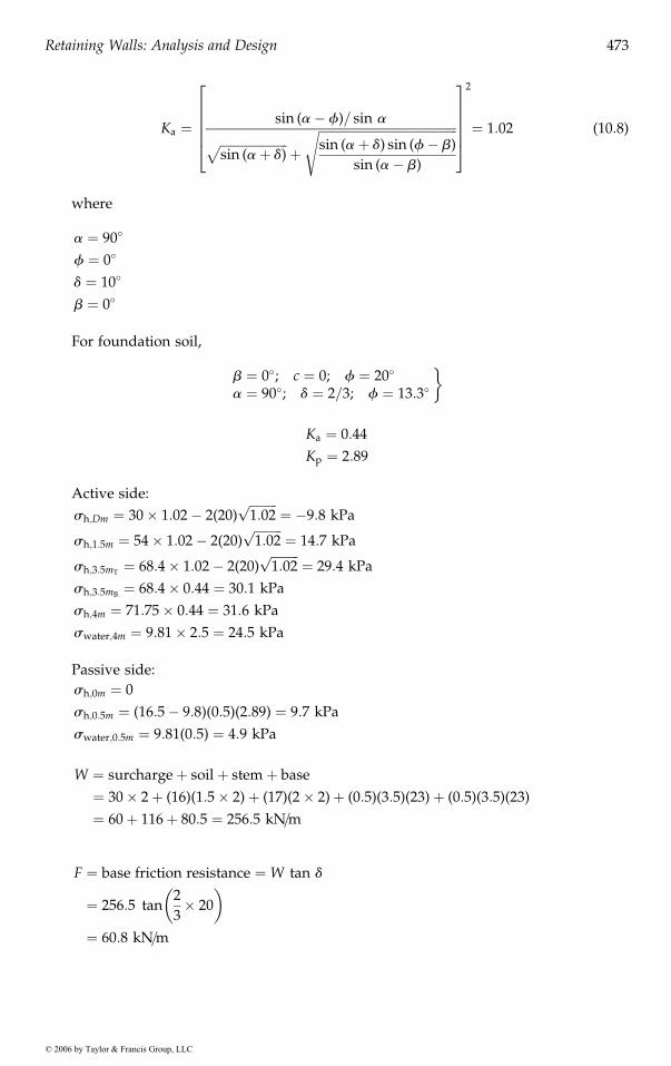
Ka ¼sin (a� f)= sin a
ffiffiffiffiffiffiffiffiffiffiffiffiffiffiffiffiffiffiffiffiffiffisin (aþ d)
pþ
ffiffiffiffiffiffiffiffiffiffiffiffiffiffiffiffiffiffiffiffiffiffiffiffiffiffiffiffiffiffiffiffiffiffiffiffiffiffiffiffiffiffiffiffiffisin (aþ d) sin (f� b)
sin (a� b)
s
266664
377775
2
¼ 1:02 (10:8)
where
a ¼ 90�
f ¼ 0�
d ¼ 10�
b ¼ 0�
For foundation soil,
b ¼ 0�; c ¼ 0; f ¼ 20�
a ¼ 90�; d ¼ 2=3; f ¼ 13:3�
�
Ka ¼ 0:44
Kp ¼ 2:89
Active side:
sh;Dm ¼ 30� 1:02� 2(20)ffiffiffiffiffiffiffiffiffi1:02p
¼ �9:8 kPa
sh;1:5m ¼ 54� 1:02� 2(20)ffiffiffiffiffiffiffiffiffi1:02p
¼ 14:7 kPa
sh;3:5mT¼ 68:4� 1:02� 2(20)
ffiffiffiffiffiffiffiffiffi1:02p
¼ 29:4 kPa
sh;3:5mB¼ 68:4� 0:44 ¼ 30:1 kPa
sh;4m ¼ 71:75� 0:44 ¼ 31:6 kPa
swater;4m ¼ 9:81� 2:5 ¼ 24:5 kPa
Passive side:
sh;0m ¼ 0
sh;0:5m ¼ (16:5� 9:8)(0:5)(2:89) ¼ 9:7 kPa
swater;0:5m ¼ 9:81(0:5) ¼ 4:9 kPa
W ¼ surchargeþ soilþ stemþ base
¼ 30� 2þ (16)(1:5� 2)þ (17)(2� 2)þ (0:5)(3:5)(23)þ (0:5)(3:5)(23)
¼ 60þ 116þ 80:5 ¼ 256:5 kN=m
F ¼ base friction resistance ¼W tan d
¼ 256:5 tan2
3� 20
� �
¼ 60:8 kN=m
Gunaratne / The Foundation Engineering Handbook 1159_C010 Final Proof page 473 22.11.2005 2:56am
Retaining Walls: Analysis and Design 473
© 2006 by Taylor & Francis Group, LLC

Active force ¼ 1
2(14:7)(0:9)þ 1
2(14:7þ 29:4)(2)þ 1
2(30:1þ 31:6)(0:5)þ 1
2(2:5)(24:5)
¼ 96:8 kN=m
Passive resistance ¼ 1
2(0:5)(9:7)þ 1
2(0:5)(4:9) ¼ 3:65 kN=m
FS ¼ 3:65þ 60:8
96:8¼ 0:66 < 1:5
So, not OK. Hence, wall will slide.
Example 10.12Check the stability of the gravity retaining wall shown in Figure 10.39(a) against over-turning and development of bottom tension.
(a) Clayey soil
Z ¼ 2C
gffiffiffiffiffiffiKa
p ¼ 2:25 m (10:11)
Su ¼ 20 kPa; g ¼ 17 kN=m; d ¼ 10�
Pax ¼ (60:56) cos 24 ¼ 55:32 kN=m
Pay ¼ (60:56) sin 24 ¼ 24:63 kN=m
(a)
Granular soilInternal friction angle = 20�Unit weight = 17.0 kN/m3
Wall friction angle = 10�
4.8 m
2 mBackfill slope = 5�
3.2 m
FIGURE 10.39Continued
Gunaratne / The Foundation Engineering Handbook 1159_C010 Final Proof page 474 22.11.2005 2:56am
474 The Foundation Engineering Handbook
© 2006 by Taylor & Francis Group, LLC

Ka ¼sin (a� f)= sin a
ffiffiffiffiffiffiffiffiffiffiffiffiffiffiffiffiffiffiffiffiffiffisin (aþ d)
pþ
ffiffiffiffiffiffiffiffiffiffiffiffiffiffiffiffiffiffiffiffiffiffiffiffiffiffiffiffiffiffiffiffiffiffiffiffiffiffiffiffiffiffiffiffiffiffisin (aþ d) sin (f� b)
sin (a� b)
s
266664
377775
2
¼ 1:095 (10:8)
Top; sh ¼ svKa � 2cffiffiffiffiffika
p
¼ �2(20)ffiffiffiffiffiffiffiffiffiffiffi1:095p
¼ �41:86 kPa
Bottom; sh ¼ (17)(4:8)(1:095)� 2(20)ffiffiffiffiffiffiffiffiffiffiffi1:095p
¼ 47:5 kPa
ww1 ¼ (2)(4:8)(23) ¼ 220:8 kN=m
Ww2¼ 1
2
� �(1:2)(4:8)(23) ¼ 66:24 kN=m
Ws ¼1
2
� �(1:2)(4:8þ 0:105)(17) ¼ 50:03 kN=m
(10:10)
4.8 m
(b)
(c)
2 m0
1.2 47.5
2.55 m
Pax
10.105 m41.86
Ww1Ww2
W3
Pa
14�10�
b = 5�
10.4
0.2
0.42c
g ka√z = = 2.15 m
Clayey soil
Pay
S4 = 20 kPa
g = 17 kN/md = 10�
Pa = (1/2) (47.5)(2.55) = 60.56
(1/3) (2.55) = 0.85 m
24�
1.2 m
1.4 m
1.6 m
Ww1
Ww2
Ws
Pay
Pax
0.85
94.3131.8
0.8
0.6
CL
14�
FIGURE 10.39(a) Illustration for Example 10.12. (b) Earth pressure calculations for Example 10.12. (c) Bottom pressuredistribution for Example 10.12.
Gunaratne / The Foundation Engineering Handbook 1159_C010 Final Proof page 475 22.11.2005 2:56am
Retaining Walls: Analysis and Design 475
© 2006 by Taylor & Francis Group, LLC

FSoverturning ¼P
Resisting momentsPOverturning moments
(taking moments at O)
¼ 220:8ð Þ(1)þ (66:24)(2þ 0:4)þ (50:03)(3:2� 0:4)þ (24:6� 3)
(55:3)(0:85)
¼ 593:66
47¼ 12:6� 1:5
(10:13)
So, OK.
(b) Bottom tension
f ¼V
A�Mc
I
V¼220:8þ66:24þ50:03þ24:6
¼361:67 kN=m
A¼ (3:2Þ(1)¼3:2 m2=m
M¼ (220:8)(0:6)þ (55:3)(0:85)� (66:24)(0:8)� (50:03)(1:2)� (24:6)(1:4)¼32:017 kNm
I¼ 6h3
12¼ (1)(3:2)3
12¼2:73
Max: stress ¼ Fmax ¼361:67
3:2þ (32)(1:6)
2:73¼ 131:8 kPa
Min: stress ¼ Fmin ¼361:67
3:2� (32)(1:6)
2:73¼ 94:3 kPa
There is no tension.
Example 10.13Investigate the stability of the cantilever sheet-pile wall shown in Figure 10.40 using thefree-earth support method. Assume that the depth embedment is 1.5 m.
Surcharge = 10 kPa
GWT,Elev. 1.5 m
Backfill ofclayey soil cohesion = 20kPaInternal frictionangle = 20�Dry unit weight= 16.0 kN/m3
Sat. unit weight= 17.0 kN/m3
Original ground of clayey soil, Sat. unit weight = 16.5 kN/m3
Undrained strength = 20 kPa
Elev. 2.5 m
Elev. 0.0
(a)
FIGURE 10.40Continued
Gunaratne / The Foundation Engineering Handbook 1159_C010 Final Proof page 476 22.11.2005 2:56am
476 The Foundation Engineering Handbook
© 2006 by Taylor & Francis Group, LLC

Right side:
sh,0m ¼ (10)(0:49)� 2(20)ffiffiffiffiffiffiffiffiffi0:49p
¼ �23:1 kPa
sh,1m ¼ (10þ 16� 1)(0:49)� 2(20)ffiffiffiffiffiffiffiffiffi0:49p
¼ �15:26 kPa
sh,2:5m ¼ (10þ 16þ (17� 9:8)(1:5))(0:49)� 2(20)ffiffiffiffiffiffiffiffiffi0:49p
¼ �9:97 kPa
sh,2:5m ¼ (36:8)(1)� 2(20)ffiffiffi1p¼ �3:2 kPa
sh,4m ¼ (36:8þ (16:5� 9:8)(1:5))(!)� 2(20)ffiffiffi1p¼ þ6:85 kPa
sh,w4m¼ (9:8)(3) ¼ 29:4 kPa
q =10 kPa
23.1
15.26
9.97 14.7
Water press
C = 20 kPa
Kp =1/ka = 2.041.0 m
1.5 m
1.5 m
(b)
f = 20�gd =16 kN/m3
ge = 16 kN/m3
gs = 16.5 kN/m3
Sa = 20 kPa
Ka = 1 = kp
Kc =1− sinf
1+ sinf= 0.49
A
q = 10 kPa
M 14.7 B
F
P3
P4
P2
P1
E N 101.55 C28.5
(c)
D1
FIGURE 10.40(a) Illustration for Example 10.13. (b) Earth pressure calculations for Example 10.13. (c) Earth pressure distribu-tion for Example 10.13.
Gunaratne / The Foundation Engineering Handbook 1159_C010 Final Proof page 477 22.11.2005 2:56am
Retaining Walls: Analysis and Design 477
© 2006 by Taylor & Francis Group, LLC

Left side:
sp,0m ¼ 2(20)ffiffiffi1p¼ 40 kPa
sp,1:5m ¼ (16:5� 9:8)(1:5)(1)þ 2(20)ffiffiffi1p¼ 50:05 kPa
sa,0m ¼ �2(20)ffiffiffi1p¼ �40 kPa
sa,1:5m ¼ (16:5� 9:8)(1:5)(1)� 2(20)ffiffiffi1p¼ 29:95 kPa
From the figure,
Horizontal stress at E, sE ¼ (50:05þ 14:7)� (6:85þ 29:4) ¼ 28:5 kPa
Horizontal stress at C, sC ¼ (86:85þ 29:4)� (14:7) ¼ 101:55 kPa
P1 ¼1
214:7ð Þ 1:5ð Þ ¼ 11:02 kN=m
P2 ¼ 14:7 1:5ð Þ ¼ 22:05 kN=m
P3 ¼1
228:5þ 14:7ð Þ 1:5ð Þ ¼ 32:4 kN=m
P4 ¼1
228:5 þ 101:55ð Þ (D1) ¼ 65:02D1
XFx ¼ 0
therefore, 11:02þ 22:05� 32:4þ 65:02D1 ¼ 0
D1 ¼ negative
Point of rotation does not exist.Wall will move rightward, Unstable.
Example 10.14Assuming that the depth of embedment is 1.2 m, estimate the magnitude of tensioningrequired for stability of the anchored sheet-pile wall shown in Figure 10.41(a). Commenton the depth of embedment provided.
Surcharge = 20 kPa
Backfill ofclayey soil cohesion = 2 kPa Internal frictionangle = 20�Unit weight =16.5 kN/m3
Wall frictionangle = 10�
T
Elev. 2.5 m
(a) Original ground of clayey soil, Unit weight = 17.5 kN/m3
Undrained strength = 10 kPa
FIGURE 10.41Continued
Gunaratne / The Foundation Engineering Handbook 1159_C010 Final Proof page 478 22.11.2005 2:56am
478 The Foundation Engineering Handbook
© 2006 by Taylor & Francis Group, LLC

da
Backfill
Original clayey soil
T
C = 2 kPa, f = 20�
Su = 10 kPa
sin(a − f )/sin(w) ]
g = 16.5 kN/m3
g = 17.5 kN/m3
d = 10�
q = 20 kPa
6.27
T
PA1
PP3
PA3
PA2
1.25
24.7
2.033
41.25
0.40.6
PP2
0.4
2
41
0.6
O
20
2.5 m
1.2 m
(b)
(c)
[
FIGURE 10.41(a) Illustration for Example 10.14. (b) Properties of different soil layers in Example 10.14. (c) Earth pressuredistribution for Example 10.14.
Gunaratne / The Foundation Engineering Handbook 1159_C010 Final Proof page 479 22.11.2005 2:56am
Retaining Walls: Analysis and Design 479
© 2006 by Taylor & Francis Group, LLC

(1) Backfill soil:
Ka ¼sin (a� f)=sin a
ffiffiffiffiffiffiffiffiffiffiffiffiffiffiffiffiffiffiffiffiffiffisin (aþ d)
pþ
ffiffiffiffiffiffiffiffiffiffiffiffiffiffiffiffiffiffiffiffiffiffiffiffiffiffiffiffiffiffiffiffiffisin (a þ d) sin (f � b)
sin (a � b)
q
264
375
2
¼ 0:447
f ¼ 20�; a ¼ 90�; d ¼ 10�; b ¼ 0�
(2) Original clayey soil:
Ka ¼ tan2 45� f
2
� �¼ tan2 45� 0ð Þ ¼ 1
Kp ¼1
Ka¼ 1
sha;0 ¼ svKa � 2CffiffiffiffiffiffiKa
p¼ (20)(0:447)� 2(2)(0:447) ¼ 6:27 kPa
sha;2:5mT¼ 20þ 16:5� 2:5ð Þ 0:447ð Þ � 2(2)
ffiffiffiffiffiffiffiffiffiffiffi0:447p
¼ 24:7 kPa
sha;2:5mB¼ 20þ 16:5� 2:5ð Þ(1)� 2(10)
ffiffiffi1p¼ 41:25 kPa
sha;3:7m ¼ 20þ 16:5� 2:5þ 17:5� 1:2ð Þ(1)� 2(10)ffiffiffi1p¼ 62:25 kPa
shp;0m ¼ svKp þ 2CffiffiffiffiffiffiKp
q¼ 0þ 2(10)
ffiffiffi1p¼ 20 kPa
shp;1:2m ¼ 17:5� 1:2ð Þ(1)þ 2(10)ffiffiffi1p¼ 41 kPa
5 m
30�
=60�
5.7 m
4 mm
Steel strip
q = 100 kPa
0.35 m
Sv = 0.7 m
Sh = 0.45 m
g = 17 kN/m3
f = 30�
Steel: sy = 250 mPa
? = t
−−
−
−
−−
−
−
−−
−
−
−−
−
−
−
−
−
−
−
−
−
−
−
+
+
+
+
+
45 +2f
FIGURE 10.42Illustration for Example 10.15.
Gunaratne / The Foundation Engineering Handbook 1159_C010 Final Proof page 480 22.11.2005 2:56am
480 The Foundation Engineering Handbook
© 2006 by Taylor & Francis Group, LLC

PA1¼ 6:27ð Þ 2:5ð Þ ¼ 15:68 kN=m
PA2¼ 1
224:7� 6:27ð Þ(2:5) ¼ 23:04 kN=m
PA3 ¼ 41:25ð Þ 1:2ð Þ ¼ 49:5 kN=m
PA4¼ 1
262:25� 41:25ð Þ (1:2) ¼ 12:6 kN=m
Pp1¼ (20)(1:2) ¼ 24 kN=m
Pp2¼ 1
241� 20ð Þ(1:2) ¼ 12:6 kN=m
XFx ¼ 0
PA ¼ Pp þ T
T ¼ 24þ 12:6ð Þ þ 15:68þ 23:04þ 9:5þ 12:6ð ÞT ¼ 64:22 kN=mX
Mo ¼ 0
T 3:7� dað Þ þ (24)(0:6)þ (12:6)(0:4) ¼ (15:68)(1:25þ 1:2)þ (23:04)(2:033)
þ (49:5)(0:6)þ (12:6)(0:4)
therefore da ¼ 2:13 m
Example 10.15A 5 m MSE wall is reinforced with steel strips at vertical and horizontal spacing of 0.7 and0.45 m, respectively. First draw the configuration of the strips and the wall. If the steelstrips are 4 mm in thickness and 5.7 m in length determine the minimum width of thestrips and the safety factor of the MSE wall against yielding under a surcharge of 100 kPa.Assume that the unit weight and internal friction are 17 kN/m3 and 308, respectively, andthe yield strength of steel is 250 MPa.
g ¼ 17 kN=m3
f ¼ 30�
Steel : sy ¼ 250 MPa
Ka ¼1� sin 30�
1þ sin 30�
¼ 0:3333
(10:2)
Maximum horizontal stresses will develop at the bottom layer
h ¼ 0:35þ 0:7� 6 ¼ 4:55 m
sa,h ¼ Kasv � 2CffiffiffiffiffiffiKa
p
¼ 0:333ð Þ 100þ 4:55� 17ð Þ ¼ 59:06 kN=m2=m
Assuming FSyielding ¼ 1:5, Fmax ¼ 1:5� 59:06� 0:7� 0:45 ¼ 27:91 kN
The width of steel stripes; w ¼ Fmax
sy � thickness¼ 27:9
250,000� 0:004¼ 0:0279 m ¼ 28 mm
Gunaratne / The Foundation Engineering Handbook 1159_C010 Final Proof page 481 22.11.2005 2:56am
Retaining Walls: Analysis and Design 481
© 2006 by Taylor & Francis Group, LLC

For bottom layer, effective length ¼ 5.7 – (5 – 4.55) tan 30 ¼ 5.44 m ¼ Le
FSpullout ¼2v � sv tan dLe
sahSvSh
¼ 1:5 ¼ 2v 100þ 4:55� 17ð Þ tan (20)(5:44)
(59:06)(0:35þ 0:45)(0:45)
therefore v ¼ 0:045 m � 45 mm
For top layer, effective length ¼ 5.7 – (5 – 0.35) tan 30 ¼ 3.02 m
2v 100þ 0:35� 17ð Þ tan (20)(3:02)
(0:333)(100þ 0:35� 17) 0:7ð Þ(0:45)¼ 1:5
therefore v ¼ 0:0715 m ¼ 71:5 mm
therefore Fsteel ¼ sy wð Þ tð Þ ¼ 250; 000 0:0715ð Þ 0:004ð Þ ¼ 71:5 kN
FSyielding ¼Fsteel
Fbottom¼ 71:5
59:06ð Þ 0:7ð Þ 0:45ð Þ ¼ 3:84 � 1:5
Glossary
Allowable stress design (ASD) — A design method in which a global factor of safety iscalculated by comparing the resisting forces to the destabilizing forces.
Earth retaining structures — A broad class of civil engineering structures intended tosupport excavations or earth fills into vertical or nearly vertical geometries.
Geosynthetic reinforced soil (GRS) — A class of MSE materials that is specificallyreinforced with geosynthetics.
Load and resistance factor design (LRFD) — A design method in which the load andresistance components are multiplied by factors related to the uncertainty associated witheach component.
Mechanically stabilized earth (MSE) — A composite material made of soil and metal,polymer, or natural fiber inclusions that exhibits superior strength and stiffness charac-teristics compared to the soil.
References
Coulomb, C.A., 1776, Essai sure une application des regles de maximis et minimis a quelquesproblemes de statique relatifs a l’architecture, Memoires de Mathematique et de Physique, pre-sented in 1773 at the Academie Royale des Sciences, 7:343–382.
Craig, R.F., 1987, Soil Mechanics, 4th edn, Van Nostrand Reinhold, New York.
Gunaratne / The Foundation Engineering Handbook 1159_C010 Final Proof page 482 22.11.2005 2:56am
482 The Foundation Engineering Handbook
© 2006 by Taylor & Francis Group, LLC

Das, B.M., 1999, Principles of Foundation Engineering, 4th edn, Brooks Cole Publishing, Pacific Grove,CA.
Fang, H.Y., ed., 1991, Foundation Engineering Handbook, 2nd edn, Van Nostrand Reinhold, New York.Holtz, R.D., Christopher, B.R., and Berg, R.R., 1997, Geosynthetic Engineering, BiTech Publishers,
Richmond, BC, Canada.Jaky, J. 1948, Earth pressure in silos, Proceedings of the Second International Conference on Soil
Mechanics and Foundation Engineering, Rotterdam, Vol. 1, pp. 103–107.Kulhawy, F.H. and Mayne, P.W., 1990, Manual on Estimating Soil Properties for Foundation Design,
Electric Power Research Insitute, Palo Alto, CA.Kulhawy, F.H., Jackson, C.S., and Mayne, P.W., 1989, First-order estimation of Ko in sands and clays,
in: Foundation Engineering: Current Principles and Practice, Kulhawy, F.H., ed., ASCE, New York,pp. 121–134.
Lacasse, S. and Lunne, T., 1988, Calibration of dilatometer correlations, Proceedings of the FirstInternational Symposium on Penetration Testing — ISOPT-1, Orlando, Vol. 1, pp. 539–548.
Marchetti, S., 1980, In-situ tests by flat dilatometer, Journal of the Geotechnical Engineering Division,ASCE, 106(GT-3):299–321.
Rankine, W.J.M., 1857, On the stability of loose earth, Philosophical Transactions of the Royal Society ofLondon, 147(Part 1):9–27.
Schmidt, B., 1966, Discussion of ‘‘Earth pressure at rest related to stress history,’’ Canadian Geotech-nical Journal, 3(4):239–242.
Seed, H.B. and Whitman, R.V., 1970, Design of earth retaining structures for dynamic loads, ASCESpecialty Conference on Lateral Stresses in the Ground and the Design of Earth-RetainingStructures, Cornell University.
Terzaghi, K., Peck, R.B., and Mesri, G., 1996, Soil Mechanics in Engineering Practice, 3rd edn, WileyInterscience, New York.
Tomlinson, M.J., 2001, Foundation Design and Construction, 7th edn, Prentice Hall, Englewood Cliffs,NJ.
Vidal, H., 1966, Terre Armee, Annales de l’Institue Technologique du Batiment et des Traveaux Publiques,France, No. 228–229, pp. 888–938.
Withiam, J.L., Voytko, E.P., Barker, R.M., Duncan, J.M., Kelly, B.C., Musser, S.C., and Elias, V., 1998,Load and resistance factor design (LRFD) of highway bridge substructures, Publication No.FHWI HI-98-032, Federal Highway Administration, Washington, DC.
Gunaratne / The Foundation Engineering Handbook 1159_C010 Final Proof page 483 22.11.2005 2:56am
Retaining Walls: Analysis and Design 483
© 2006 by Taylor & Francis Group, LLC