Embed Size (px)
Citation preview
10 Gb/s per user ultra-dense MB-OFDM metro-access
networks employing an off-the-shelf SSB generator
Daniel dos Santos Silvestre
Dissertation to obtain the Master of Science Degree in
Electrical and Computer Engineering
Supervisors: Prof. Adolfo da Visitação Tregeira Cartaxo
Dr. Tiago Manuel Ferreira Alve
Examination Committee
Chairperson: Prof. José Eduardo Charters Ribeiro da Cunha Sanguino
Supervisor: Prof. Adolfo da Visitação Tregeira Cartaxo
Member of Committee: Prof. Manuel Alberto Reis de Oliveira Violas
September 2016


iii
Acknowledgements
Acknowledgements
I would like to start by expressing my gratitude to Prof. Adolfo Cartaxo and Dr. Tiago Alves for all
the support and reviews, during the development of this dissertation. It was an unparalleled
supervision, which will certainly influence my career as a better professional.
I would like to recognise my colleagues from the optics laboratory of Instituto de
Telecomunicações, namely Pedro Cruz and Ricardo Soeiro. Many thanks for the shared knowledge
and coffee breaks.
I would also like to thank all my friends for their everlasting motivation and cherished experiences,
particularly Ângelo Sousa, Fábio Rodrigues, Inês Guimarães, Pedro Curião, Sara Gomes, Soraia
Oliveira, and every member of Casa do Povo.
Last but not least, I would like give a special thanks to my parents, António Silvestre and Adelaide
Santos, and the rest of my family for their care and endurance during my academic years.

v
Abstract
Abstract
The main objective of this dissertation is to assess the performance of a metro-access network,
which uses an intensity modulator to generate a multi-band orthogonal frequency-division multiplexing
(OFDM) optical signal, capable of ensuring 10 Gb/s per user. In order to mitigate the chromatic
dispersion induced power fading, we aim to produce a single sideband (SSB) optical signal. Therefore,
this work studies the Mach-Zehnder modulator (MZM) followed by an optical filter (OF), to select the
upper sideband of the signal spectrum. This system has the particularity of using direct detection; as a
result, an iterative algorithm for mitigation of the signal-signal beat interference is implemented.
Considering the application of an ultra-dense wavelength-division multiplexing scheme, it is fixed a
band spacing of 3.125 GHz. Regarding the transmitter, we have established to transmit 4 OFDM
bands per MZM, in order to reduce the nonlinear distortion imposed on the signal by the modulator. It
was concluded that, due to the use of virtual carriers (electrically generated in the OFDM transmitter),
the MZM must operate at the minimum bias point, and it was achieved an optimum modulation index
of 8%.
The optimization of the OF, employed to generate the SSB signal, is simulated in MATLAB®, via
software developed by the author. It includes the assessment of rectangular, 2nd
and 4th order super-
Gaussian (SG) filters, and uses the bit error rate (BER) as the figure of merit to assist in the
assessment of the receiver sensitivity. The results allow us to conclude that, with a 2nd
order SG filter,
the receiver is not able to achieve a BER of 3.8×10⁻³
, due to the poor selectivity of the filter. With a 4th
order SG filter, this metro-access network can guarantee a band capacity of 10 Gb/s to 24 users,
which is half of the value obtained for the same network configuration and using rectangular filters.
This number of users is achieved for the worst case of the network, i.e. a metro network with six 10 km
long spans and access network with 10 km reach.
Keywords: metro-access network, Mach-Zehnder modulator, orthogonal frequency-division
multiplexing, multi-band, single sideband, direct detection, virtual carrier, signal-signal beat
interference.

vii
Resumo
Resumo
O principal objectivo desta dissertação é avaliar o desempenho duma rede de metro-acesso, que
utiliza um modulador de intensidade para gerar um sinal óptico multi-banda de multiplexagem por
divisão ortogonal na frequência (OFDM), capaz de garantir 10 Gb/s por utilizador. De forma a
combater a redução de potência induzida pela dispersão cromática, pretende-se gerar um sinal óptico
de banda lateral única (SSB). Para isso, este trabalho estuda o modulador de Mach-Zehnder (MZM)
seguido de um filtro óptico (OF), para selecionar a banda lateral superior do espectro do sinal. Este
sistema tem a particularidade de usar detecção directa; desta maneira, um algoritmo iterativo de
mitigação da interferência do batimento sinal-sinal é implementado.
Tendo em conta a utilização dum esquema ultra-denso de multiplexagem por divisão do
comprimento de onda, é fixado um espaçamento entre bandas de 3.125 GHz. A respeito do emissor,
foi estabelecido transmitir 4 bandas OFDM por MZM, de forma a minimizar a distorção causada pelas
não-linearidades do modulador. Concluiu-se que, devido à utilização de portadoras virtuais (geradas
electricamente no emissor OFDM), o MZM deverá operar no ponto mínimo, e foi obtido um índice de
modulação óptimo de 8%.
A optimização do OF, empregue para produzir o sinal SSB, é simulada em MATLAB®, através de
software desenvolvido pelo autor. Esta inclui a avaliação de filtros rectangulares ideais, super-
Gaussianos (SG) de 2ª e 4ª ordem, e utiliza a taxa de erro de bit (BER) como figura de mérito no
cálculo da sensibilidade do receptor. Os resultados permitem-nos concluir que, utilizando um filtro SG
de 2ª ordem, o receptor não consegue descodificar o sinal de forma a atingir a BER de 3.8x10⁻³
,
devido à fraca selectividade do filtro. Já no caso do filtro SG de 4ª ordem, esta rede de metro-acesso
permite garantir uma capacidade de banda de 10 Gb/s a 24 utilizadores, que é metade do alcançado
para a mesma configuração de rede e utilizando filtros rectangulares. Este número de utilizadores é
conseguido para o pior caso da rede, ou seja, é dividido por seis nós equidistantes numa rede
metropolitana com 60 km e rede de acesso com 10 km de comprimento.
Palavras-chave: rede de metro-acesso, modulador de Mach-Zehnder, multiplexagem por divisão
ortogonal na frequência, multi-banda, banda lateral única, detecção directa, portadora virtual,
interferência do batimento sinal-sinal.

ix
Table of Contents
Table of Contents
Acknowledgements ............................................................................................................................ iii
Abstract ...............................................................................................................................................v
Resumo ............................................................................................................................................. vii
Table of Contents ............................................................................................................................... ix
List of Figures ..................................................................................................................................... xi
List of Tables .................................................................................................................................... xiii
List of Acronyms ................................................................................................................................ xv
List of Symbols ................................................................................................................................. xix
Introduction .............................................................................................................................. 1 1
1.1 Scope of the work ............................................................................................................. 2
1.1.1 Optical networks .................................................................................................... 2 1.1.2 Metro-access network ........................................................................................... 3 1.1.3 Optical transmitter and receiver ............................................................................. 4 1.1.4 Orthogonal frequency-division multiplexing concept ............................................. 6 1.1.5 MB-OFDM concept ................................................................................................ 7
1.2 Motivation ......................................................................................................................... 8
1.3 Objectives and structure of the dissertation ..................................................................... 8
1.4 Main original contributions ................................................................................................ 9
Description of the MB-OFDM system .................................................................................... 11 2
2.1 OFDM signal basics ....................................................................................................... 12
2.1.1 Mathematical formulation of an MCM signal ....................................................... 12 2.1.2 Discrete Fourier transform ................................................................................... 12 2.1.3 Cyclic prefix ......................................................................................................... 13 2.1.4 Spectral efficiency................................................................................................ 14 2.1.5 Peak-to-average power ratio ............................................................................... 16
2.2 Optical OFDM communication system ........................................................................... 16
2.2.1 OFDM Transmitter ............................................................................................... 16 2.2.2 OFDM Receiver ................................................................................................... 18
2.3 SSB signal generator ..................................................................................................... 20
2.3.1 Mach-Zehnder modulator .................................................................................... 20 2.3.2 Single sideband-optical filter ................................................................................ 22
2.4 MB-OFDM signal basics ................................................................................................. 23
2.5 Virtual carrier-assisted MB-OFDM signal ....................................................................... 25
2.5.1 Virtual carrier-to-band power ratio ....................................................................... 26

x
2.5.3 Virtual carrier-to-band gap ................................................................................... 27 2.5.4 Iterative SSBI mitigation algorithm ...................................................................... 27
2.6 MB-OFDM metro-access network .................................................................................. 32
2.6.1 Central office and optical line terminal................................................................. 32 2.6.2 Remote unit and OA ............................................................................................ 33 2.6.1 Optical network unit ............................................................................................. 33
2.7 Conclusion ...................................................................................................................... 34
Optimization of the parameters of the MB-OFDM system ..................................................... 35 3
3.1 Introduction ..................................................................................................................... 36
3.2 Modulation scheme ........................................................................................................ 36
3.3 Cyclic prefix .................................................................................................................... 38
3.4 Virtual carrier-to-band gap .............................................................................................. 38
3.5 Virtual carrier-to-band power ratio .................................................................................. 39
3.6 Bandwidth and detuning of the BS ................................................................................. 40
3.7 Bias point and MI of the MZM ........................................................................................ 42
3.8 Length of the spans ........................................................................................................ 44
3.9 Conclusion ...................................................................................................................... 46
SSB-OF optimization and power budget assessment ........................................................... 49 4
4.1 System setup description ............................................................................................... 50
4.2 Power budget with rectangular filters ............................................................................. 51
4.3 2nd
order SG SSB-OF optimization................................................................................. 52
4.4 Power budget with the 2nd
order SG SSB-OF ................................................................ 55
4.5 4th order SG SSB-OF optimization ................................................................................. 57
4.6 Power budget with the 4th order SG SSB-OF ................................................................. 59
4.7 Conclusion ...................................................................................................................... 60
Conclusion ............................................................................................................................. 63 5
5.1 Final conclusions ............................................................................................................ 64
5.2 Future Works .................................................................................................................. 65
References ....................................................................................................................................... 67
A. OFDM system details ............................................................................................................. 71
B. Performance evaluation methods .......................................................................................... 77
xi
List of Figures
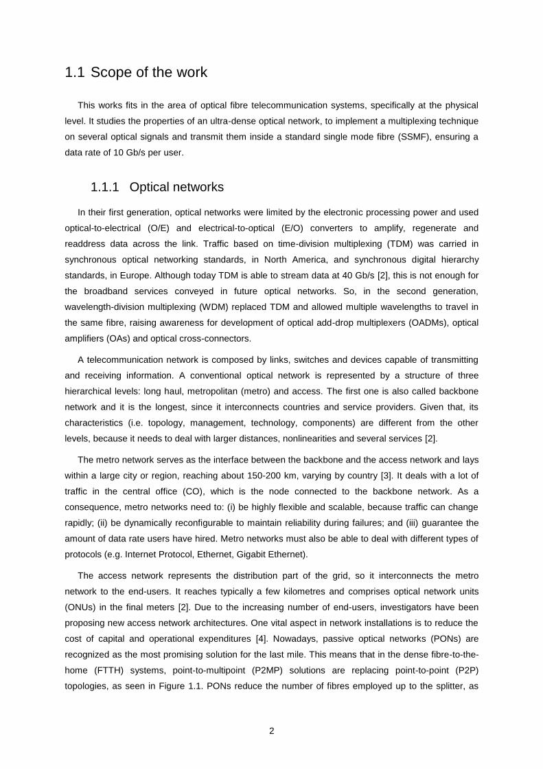
List of Figures Figure 1.1: FTTH topologies: (a) P2P; (b) P2MP. .................................................................................... 3
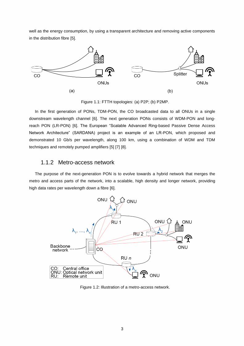
Figure 1.2: Illustration of a metro-access network. .................................................................................. 3
Figure 1.3: Illustration of the CDIPF effect on: (a) a DSB signal; (b) an SSB signal................................ 5
Figure 1.4: Example of the band routing in an add-drop node. ................................................................ 7
Figure 2.1: Time waveform of the in-phase part of an OFDM symbol, with insertion of CP. .................14
Figure 2.2: Illustrative OFDM signal spectrum with five orthogonal subcarriers. ...................................15
Figure 2.3: Spectrum of a baseband OFDM symbol. .............................................................................16
Figure 2.4: OFDM SSB transmitter architecture using up-conversion. ..................................................17
Figure 2.5: Spectrum of a passband DSB OFDM symbol. .....................................................................18
Figure 2.6: DD-OFDM receiver architecture using down-conversion. ...................................................19
Figure 2.7: Illustration of a Mach-Zehnder modulator and a CWL source. ............................................20
Figure 2.8: Field transfer characteristic of the MZM, with Vπ = 5 V. .......................................................22
Figure 2.9: Amplitude response of (a) Gaussian filter and (b) 2nd order SG filter. ................................23
Figure 2.10: Illustration of the MB-OFDM signal inside one channel. ....................................................23
Figure 2.11: Illustration of an SSB signal spectrum at the PIN PD (a) input and (b) output. .................25
Figure 2.12: Illustration of the MB-OFDM signal using VCs and its frequency parameters. ..................26
Figure 2.13: Feedback loop of the SSBI mitigation algorithm. ...............................................................28
Figure 2.14: Evolution of the EVM as a function of (a) the SSBI iterations and particularly for (b)
the Γc iterations inside each SSBI iteration. ............................................................................30
Figure 2.15: Normalized PSD of the signal at: (a) store module A; (b) final step of store module
C; and (c) final step of store module B. ...................................................................................31
Figure 2.16: QAM symbols at the (a) input and (b) output of the SSBI mitigation algorithm. ................32
Figure 2.17: Block diagram of the downstream MB-OFDM metro-access network. ..............................33
Figure 2.18: ROADM inside the RU (for downstream only). ..................................................................34
Figure 3.1: Illustration of the amplitude response of a 2nd
order SG BS (in blue), selecting a
16-QAM OFDM band and part of the previous pair band-VC. ................................................37
Figure 3.2: Illustration of the amplitude response of a 2nd
order SG BS (in blue), selecting a
32-QAM OFDM band. .............................................................................................................37
Figure 3.3: EVM as a function of the normalized VBG, for a 32-QAM OFDM band. .............................39
Figure 3.4: EVM as a function of the VBPR, with OSNR = 30 dB. .........................................................40
Figure 3.5: Representation of an MB-OFDM signal spectrum before the BS. .......................................40
Figure 3.6: Normalized PSDs of the signal before and after the BS. .....................................................41
Figure 3.7: EVM as a function of the subcarriers. ..................................................................................41
Figure 3.8: EVM, in decibel, of the middle band of a (a) 3-band, (b) 5-band, (c) 7-band and 9-
band OFDM system, as a function of the detuning and -3 dB bandwidth of the 2nd
xii
order SG BS. ...........................................................................................................................42
Figure 3.9: EVM as a function of the MI for 1, 2 and 4 OFDM bands transmitted per MZM. .................44
Figure 3.10: EVM as a function of the length of the span, transmitting (a) 1 band and (b) 4
bands (EVM of the 3rd
band). ..................................................................................................45
Figure 4.1: Illustration of the upper sideband spectrum at the output of the “MB-OFDM Tx”. ...............50
Figure 4.2: BER levels of the 3rd
band of a signal that travels along (a) one span and (b) six
spans, when using rectangular filters for the SSB-OF and BS. ..............................................51
Figure 4.3: PSD of channel A and B, at the output of the 2nd
order SG filter. ........................................53
Figure 4.4: EVM, in decibel, of (a) band 1 and (b) band 4 of channel A, as a function of the
detuning and -3 dB bandwidth of the 2nd
order SG SSB-OF. .................................................54
Figure 4.5: PSD of channel A at the input and output of the 2nd
order SSB-OF with optimized
features. ..................................................................................................................................55
Figure 4.6: BER levels of each band for six spans of (a) 25 km and (b) 10 km, when using 2nd
order SG filters for the SSB-OF. .............................................................................................56
Figure 4.7: PSD of channel A and B, at the output of the 4th order SG filter. .........................................57
Figure 4.8: EVM, in decibel, of (a) band 1 and (b) band 4 of channel A, as a function of the
detuning and -3 dB bandwidth of the 4th order SG SSB-OF ...................................................58
Figure 4.9: OFDM spectrum of channel A before and after the 4th order SSB-OF with optimized
features. ..................................................................................................................................59
Figure 4.10: BER levels of each band for six spans of (a) 15 km and (b) 10 km, when using 4th
order SG filters for the SSB-OF. .............................................................................................60
Figure A.1: 16-QAM ideal constellation. .................................................................................................73
Figure A.2: 16-QAM constellation at the equalizer input. .......................................................................73
Figure A.3: 16-QAM constellation at the equalizer output. .....................................................................73
Figure A.4: Equivalent circuit for the front-end. ......................................................................................74
Figure B.1: Illustration of the EVM of one constellation symbol. ............................................................78
Figure B.2: BER as a function of the number of noise runs, by the EGA method. ................................79

xiii
List of Tables
List of Tables Table 3.1: OFDM bandwidth for different modulation schemes. ............................................................36
Table 3.2: Parameters of the signal and the SSMF. ..............................................................................38
Table 3.3: Parameters of a 32-QAM OFDM symbol. .............................................................................38
Table 3.4: Parameters of some elements inside the metro-access network. ........................................43
Table 3.5: Maximum length of spans to ensure a BER of 3.8×10⁻³
........................................................46
Table 3.6: Numerical parameters of the MB-OFDM system. .................................................................47
Table 4.1: Power budget of the access network and maximum number of users per RU-node,
when using rectangular filters for the SSB-OF and BS, in a metro network with six
spans. ......................................................................................................................................52
Table 4.2: Power budget of the access network and maximum number of users per RU-node,
when using 4th order SG SSB-OFs and 2
nd order SG order BS, in a metro network with
six spans. ................................................................................................................................60


xv
List of Acronyms
List of Acronyms A
ADC Analogue-to-digital converter
B
B2B Back-to-back
BER Bit error rate
BS Band selector
C
CD Chromatic dispersion
CDIPF Chromatic dispersion induced power fading
CO Central office
CO-OFDM Coherent optical orthogonal frequency-division multiplexing
CP Cyclic prefix
CWL Continuous wave laser
D
DAC Digital-to-analogue converter
DC Direct current
DD Direct-detection
DD-OFDM Direct-detection orthogonal frequency-division multiplexing
DFT Discrete Fourier transform
DSB Double sideband
DSP Digital signal processing
DWDM Dense wavelength-division multiplexing
E
E/O Electrical-to-optical
EPoA Electrical post-amplifier
EPrA Electrical pre-amplifier
EVM Error vector magnitude
F
FEC Forward error correction
FFT Fast Fourier transform
xvi
FTTH Fibre-to-the-home
FWM Four-wave mixing
I
IDFT Inverse discrete Fourier transform
IFFT Inverse fast Fourier transform
IM Intensity modulator
ISI Intersymbol interference
L
LPF Low-pass filter
LR-PON Long-reach passive optical network
M
MB-OFDM Multi-band orthogonal frequency-division multiplexing
MBP Minimum bias point
MCM Multi-carrier modulation
MI Modulation index
MORFEUS Metro networks based on multi-band orthogonal frequency-division multiplexing signals
MUX Multiplexer
MZM Mach-Zehnder modulator
O
O/E Optical-to-electrical
OA Optical amplifier
OADM Optical add-drop multiplexer
OF Optical filter
OFDM Orthogonal frequency-division multiplexing
OLT Optical line terminal
ONU Optical network unit
OSNR Optical signal-to-noise ratio
P
P/S Parallel-to-serial
P2MP Point-to-multipoint
P2P Point-to-point
PAPR Peak-to-average power ratio
PD Photodiode
PIN Positive-intrinsic-negative
PON Passive optical network

xvii
PSD Power spectral density
PSK Phase-shift keying
Q
QAM Quadrature amplitude modulation
QBP Quadrature bias point
R
RF Radio-frequency
RMS Root mean square
ROADM Reconfigurable optical add-drop multiplexer
RU Remote unit
Rx Receiver
S
S/P Serial-to-parallel
SARDANA Scalable advanced ring-based passive dense access network
SG Super-Gaussian
SSB Single sideband
SSB-OF Single sideband-optical filter
SSBI Signal-signal beat interference
SSMF Standard single mode fibre
T
TDM Time-division multiplexing
Tx Transmitter
V
VBG Virtual carrier-to-band gap
VBPR Virtual carrier-to-band power ratio
VC Virtual carrier
W
WDM Wavelength-division multiplexing


xix
List of Symbols
List of Symbols
Γc transmission coefficient
S
half-power spectral width of the optical signal
gf
optical carrier-to-band gap
scf
frequency spacing of OFDM subcarriers
cB
frequency gap in-between DWDM channels
gB
frequency gap in-between OFDM bands
spectral efficiency
λ
optical wavelength
0
nominal optical wavelength
0 nominal optical frequency
t
pulse shaping function
T
standard deviation of the thermal noise current
∥
parallel polarisation in the fibre
⊥ perpendicular polarisation in the fibre
A
optical carrier amplitude
3dBB
bandwidth at -3 dB of an optical filter
20dBB
bandwidth at -20 dB of an optical filter
chB
bandwidth of the DWDM channel
Be bandwidth of the electrical noise
MB OFDMB
bandwidth of the MB-OFDM signal
OFDMB
bandwidth of the OFDM signal
SB
bandwidth of the frequency slots
WDMB
total bandwidth of the MB-OFDM signals
c
speed of light in vacuum
xx
,k ic
i-th information symbol at the k-th subcarrier
0D
fibre dispersion parameter at wavelength 0
ine t
optical field of the signal at the photodetector input
oute t
optical field of the signal at the MZM output
,OA ine t
optical field of the signal at the optical amplifier input
,OA oute t
optical field of the signal at the optical amplifier output
inE
optical field at the MZM input
1,1f
central frequency of the first OFDM band of channel 1
1,if
central frequency of the i-th OFDM band of channel 1
,j if
central frequency of the i-th OFDM band of channel j
kf
frequency of the k-th subcarrier
,j ivcf
frequency of the virtual carrier corresponding to the i-th OFDM band of channel j
fn
noise figure of the amplifier
RFf
central frequency of the up-converted OFDM signal
g gain of the amplifier
h Planck constant
( )ichH k
channel transfer function of the i-th OFDM training symbol
,ch SSBIH k channel transfer function for the SSBI mitigation algorithm
eqH k
equalizer transfer function
lossi
optical power insertion loss of the MZM
outi t
current at the front-end receiver output
,tr signali t
signal ,tr SSB OFDMi t without the SSBI term
,tr SSB OFDMi t
stored OFDM training signal
,tr SSBIi t
SSBI term of ,tr SSB OFDMi t
,tr SSBI freei t
OFDM training signal at the output of the SSBI mitigation algorithm
,ˆtr SSBIi t
estimated SSBI term of ,tr SSB OFDMi t
PINi t
current at the photodetector output
Ti t
thermal noise current at the front-end receiver
ˆSSBIi t
estimated SSBI term at the output of the square law operator
I in-phase component of a OFDM signal
Bk
Boltzmann constant
L
length of the fibre

xxi
m
modulation index of the MZM
M
number of modulation symbols in QAM mapping
ASEn t
ASE noise
bN
number of slots inside a DWDM channel
cN
number of DWDM channels
scN
number of subcarriers
spN
number of spans inside the metro network
bp
average power of the OFDM band
inp t
optical power of the incident light at the photodetector input
outp t
optical power at the MZM output
vcp
average power of the virtual carrier
inP
optical power at the MZM input
Q quadrature component of a OFDM signal
R
responsivity of the photodetector
bR
bit rate of the OFDM signal
MB OFDMbR
bit rate of the MB-OFDM signal
WDMbR
bit rate of the system
LR
load resistance
s n
n-th sample of the transmitted symbol s t
s t transmitted OFDM baseband signal
s t
received OFDM baseband signal
,b norms t
sum of all the up-converted OFDM signals after normalization of the RMS voltage
ks
waveform for the k-th subcarrier
ips k
k-th QAM symbol of the i-th transmitted OFDM training symbol
lrxs k
QAM symbol of the k-th subcarrier of the l-th received OFDM symbol
i
ts k
k-th QAM symbol of the i-th received OFDM training symbol
l
txs k
QAM symbol of the k-th subcarrier of the l-th transmitted OFDM symbol
RFs t
transmitted OFDM signal at frequency RFf
RFs t
received OFDM signal at frequency RFf
fS
selectivity of an optical filter
ASES
power spectral density of the ASE noise
TS f
power spectral density of the thermal noise

xxii
t
time
dt
time delay
T standard noise temperature
tT
OFDM symbol period with CP
gT
CP period
ST
OFDM symbol period
acv
electrical signal at the MZM arm input
normv t
sum of all the up-converted virtual carriers after normalization of the RMS voltage
V
switching voltage of the MZM
biasV
bias voltage of the MZM
RMSV
root mean square voltage of acv

1
Chapter 1
Introduction
Introduction 1
2
1.1 Scope of the work
This works fits in the area of optical fibre telecommunication systems, specifically at the physical
level. It studies the properties of an ultra-dense optical network, to implement a multiplexing technique
on several optical signals and transmit them inside a standard single mode fibre (SSMF), ensuring a
data rate of 10 Gb/s per user.
1.1.1 Optical networks
In their first generation, optical networks were limited by the electronic processing power and used
optical-to-electrical (O/E) and electrical-to-optical (E/O) converters to amplify, regenerate and
readdress data across the link. Traffic based on time-division multiplexing (TDM) was carried in
synchronous optical networking standards, in North America, and synchronous digital hierarchy
standards, in Europe. Although today TDM is able to stream data at 40 Gb/s [2], this is not enough for
the broadband services conveyed in future optical networks. So, in the second generation,
wavelength-division multiplexing (WDM) replaced TDM and allowed multiple wavelengths to travel in
the same fibre, raising awareness for development of optical add-drop multiplexers (OADMs), optical
amplifiers (OAs) and optical cross-connectors.
A telecommunication network is composed by links, switches and devices capable of transmitting
and receiving information. A conventional optical network is represented by a structure of three
hierarchical levels: long haul, metropolitan (metro) and access. The first one is also called backbone
network and it is the longest, since it interconnects countries and service providers. Given that, its
characteristics (i.e. topology, management, technology, components) are different from the other
levels, because it needs to deal with larger distances, nonlinearities and several services [2].
The metro network serves as the interface between the backbone and the access network and lays
within a large city or region, reaching about 150-200 km, varying by country [3]. It deals with a lot of
traffic in the central office (CO), which is the node connected to the backbone network. As a
consequence, metro networks need to: (i) be highly flexible and scalable, because traffic can change
rapidly; (ii) be dynamically reconfigurable to maintain reliability during failures; and (iii) guarantee the
amount of data rate users have hired. Metro networks must also be able to deal with different types of
protocols (e.g. Internet Protocol, Ethernet, Gigabit Ethernet).
The access network represents the distribution part of the grid, so it interconnects the metro
network to the end-users. It reaches typically a few kilometres and comprises optical network units
(ONUs) in the final meters [2]. Due to the increasing number of end-users, investigators have been
proposing new access network architectures. One vital aspect in network installations is to reduce the
cost of capital and operational expenditures [4]. Nowadays, passive optical networks (PONs) are
recognized as the most promising solution for the last mile. This means that in the dense fibre-to-the-
home (FTTH) systems, point-to-multipoint (P2MP) solutions are replacing point-to-point (P2P)
topologies, as seen in Figure 1.1. PONs reduce the number of fibres employed up to the splitter, as
3
well as the energy consumption, by using a transparent architecture and removing active components
in the distribution fibre [5].
Figure 1.1: FTTH topologies: (a) P2P; (b) P2MP.
In the first generation of PONs, TDM-PON, the CO broadcasted data to all ONUs in a single
downstream wavelength channel [6]. The next generation PONs consists of WDM-PON and long-
reach PON (LR-PON) [6]. The European “Scalable Advanced Ring-based Passive Dense Access
Network Architecture” (SARDANA) project is an example of an LR-PON, which proposed and
demonstrated 10 Gb/s per wavelength, along 100 km, using a combination of WDM and TDM
techniques and remotely pumped amplifiers [5] [7] [8].
1.1.2 Metro-access network
The purpose of the next-generation PON is to evolve towards a hybrid network that merges the
metro and access parts of the network, into a scalable, high density and longer network, providing
high data rates per wavelength down a fibre [6].
Figure 1.2: Illustration of a metro-access network.
4
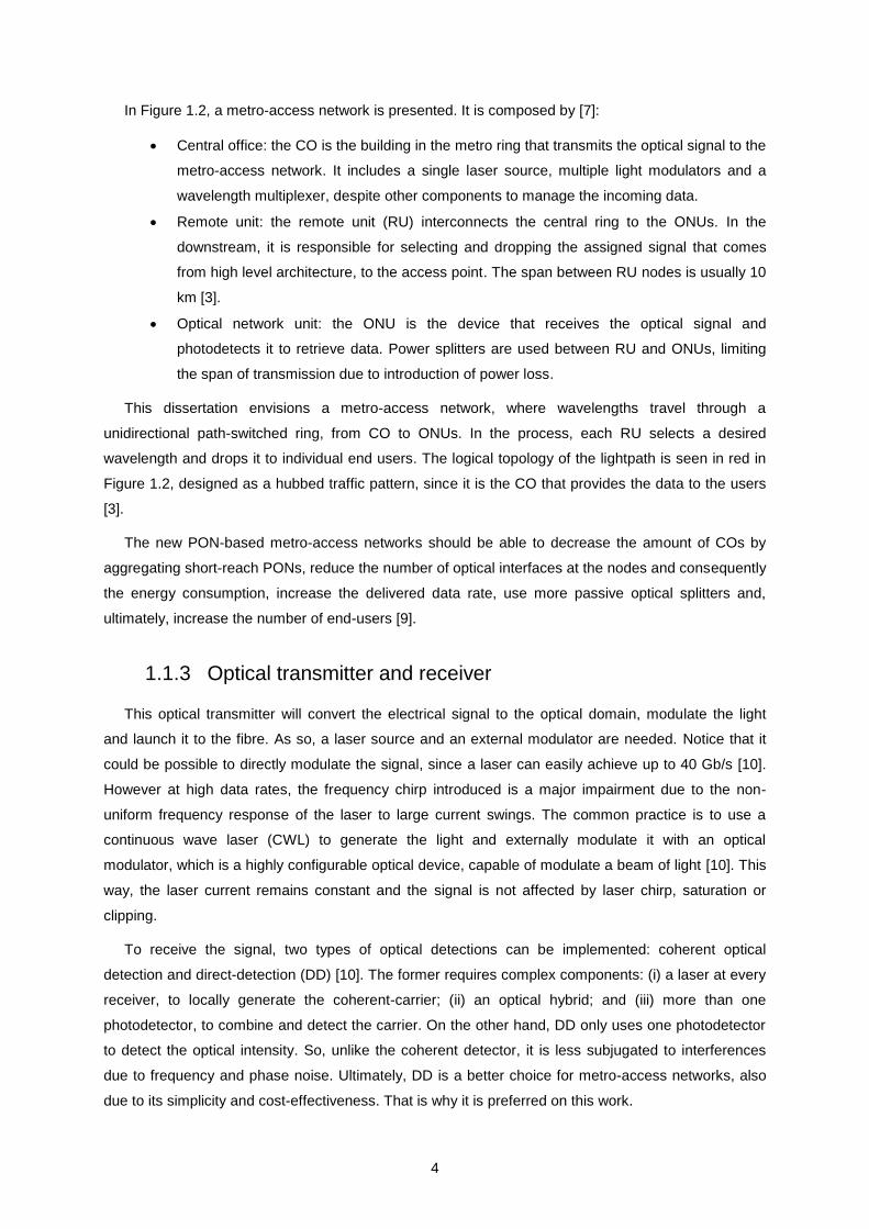
In Figure 1.2, a metro-access network is presented. It is composed by [7]:
Central office: the CO is the building in the metro ring that transmits the optical signal to the
metro-access network. It includes a single laser source, multiple light modulators and a
wavelength multiplexer, despite other components to manage the incoming data.
Remote unit: the remote unit (RU) interconnects the central ring to the ONUs. In the
downstream, it is responsible for selecting and dropping the assigned signal that comes
from high level architecture, to the access point. The span between RU nodes is usually 10
km [3].
Optical network unit: the ONU is the device that receives the optical signal and
photodetects it to retrieve data. Power splitters are used between RU and ONUs, limiting
the span of transmission due to introduction of power loss.
This dissertation envisions a metro-access network, where wavelengths travel through a
unidirectional path-switched ring, from CO to ONUs. In the process, each RU selects a desired
wavelength and drops it to individual end users. The logical topology of the lightpath is seen in red in
Figure 1.2, designed as a hubbed traffic pattern, since it is the CO that provides the data to the users
[3].
The new PON-based metro-access networks should be able to decrease the amount of COs by
aggregating short-reach PONs, reduce the number of optical interfaces at the nodes and consequently
the energy consumption, increase the delivered data rate, use more passive optical splitters and,
ultimately, increase the number of end-users [9].
1.1.3 Optical transmitter and receiver
This optical transmitter will convert the electrical signal to the optical domain, modulate the light
and launch it to the fibre. As so, a laser source and an external modulator are needed. Notice that it
could be possible to directly modulate the signal, since a laser can easily achieve up to 40 Gb/s [10].
However at high data rates, the frequency chirp introduced is a major impairment due to the non-
uniform frequency response of the laser to large current swings. The common practice is to use a
continuous wave laser (CWL) to generate the light and externally modulate it with an optical
modulator, which is a highly configurable optical device, capable of modulate a beam of light [10]. This
way, the laser current remains constant and the signal is not affected by laser chirp, saturation or
clipping.
To receive the signal, two types of optical detections can be implemented: coherent optical
detection and direct-detection (DD) [10]. The former requires complex components: (i) a laser at every
receiver, to locally generate the coherent-carrier; (ii) an optical hybrid; and (iii) more than one
photodetector, to combine and detect the carrier. On the other hand, DD only uses one photodetector
to detect the optical intensity. So, unlike the coherent detector, it is less subjugated to interferences
due to frequency and phase noise. Ultimately, DD is a better choice for metro-access networks, also
due to its simplicity and cost-effectiveness. That is why it is preferred on this work.
5
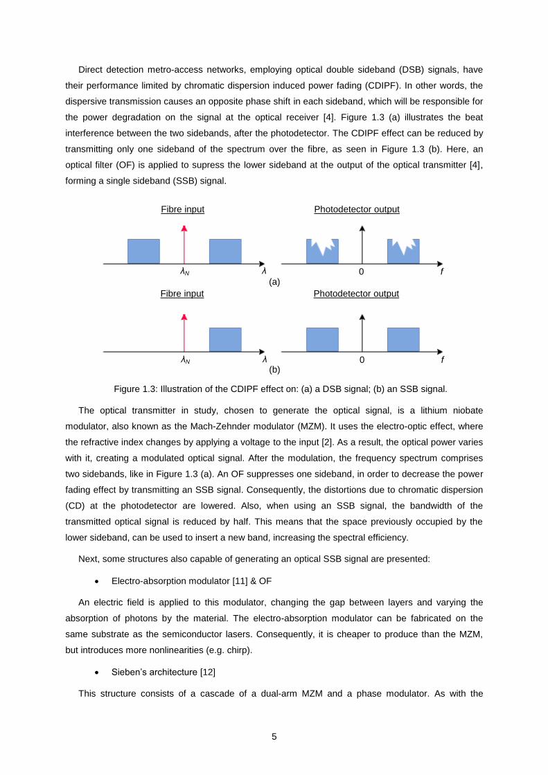
Direct detection metro-access networks, employing optical double sideband (DSB) signals, have
their performance limited by chromatic dispersion induced power fading (CDIPF). In other words, the
dispersive transmission causes an opposite phase shift in each sideband, which will be responsible for
the power degradation on the signal at the optical receiver [4]. Figure 1.3 (a) illustrates the beat
interference between the two sidebands, after the photodetector. The CDIPF effect can be reduced by
transmitting only one sideband of the spectrum over the fibre, as seen in Figure 1.3 (b). Here, an
optical filter (OF) is applied to supress the lower sideband at the output of the optical transmitter [4],
forming a single sideband (SSB) signal.
Figure 1.3: Illustration of the CDIPF effect on: (a) a DSB signal; (b) an SSB signal.
The optical transmitter in study, chosen to generate the optical signal, is a lithium niobate
modulator, also known as the Mach-Zehnder modulator (MZM). It uses the electro-optic effect, where
the refractive index changes by applying a voltage to the input [2]. As a result, the optical power varies
with it, creating a modulated optical signal. After the modulation, the frequency spectrum comprises
two sidebands, like in Figure 1.3 (a). An OF suppresses one sideband, in order to decrease the power
fading effect by transmitting an SSB signal. Consequently, the distortions due to chromatic dispersion
(CD) at the photodetector are lowered. Also, when using an SSB signal, the bandwidth of the
transmitted optical signal is reduced by half. This means that the space previously occupied by the
lower sideband, can be used to insert a new band, increasing the spectral efficiency.
Next, some structures also capable of generating an optical SSB signal are presented:
Electro-absorption modulator [11] & OF
An electric field is applied to this modulator, changing the gap between layers and varying the
absorption of photons by the material. The electro-absorption modulator can be fabricated on the
same substrate as the semiconductor lasers. Consequently, it is cheaper to produce than the MZM,
but introduces more nonlinearities (e.g. chirp).
Sieben’s architecture [12]
This structure consists of a cascade of a dual-arm MZM and a phase modulator. As with the
Fibre input Photodetector output
λN λ
Fibre input Photodetector output
0 f
0 f λN λ
(a)
(b)
6
structure in study, the MZM serves as an external intensity modulator (IM). The resulting optical DSB
signal is fed to a phase modulator that modifies the input, resulting in an SSB signal.
Dual-Parallel MZM [13]
This structure consists of two MZMs embedded in a main dual-arm MZM, to control the phase
between the optical fields of the inner MZMs. This arrangement allows generating an SSB signal
without resorting to optical filtering. Nevertheless, the less intricate and less costly MZM & OF scheme
will be assessed in this work.
1.1.4 Orthogonal frequency-division multiplexing concept
In telecommunications there are two essential techniques for digital modulation. One uses a single
main carrier and, in the other, data is broadcast through multiple subcarriers (e.g. WDM).
At high data rate, single-carrier modulation needs short symbol period. In a real channel, these
symbols would eventually expand and produce intersymbol interference (ISI), due to channel
dispersion. To overcome ISI, in multi-carrier modulation (MCM) we make the symbol period higher
than the delay spread of the channel [4]. This would seem like an inefficient practice, but since MCM
uses multiple carriers in parallel, the effective data rates turn out to be higher than the ones in single-
carrier modulation. Orthogonal frequency-division multiplexing (OFDM) is an MCM scheme, in which a
single band comprises multiple subcarriers on equally spaced adjacent frequencies [10]. These
subcarriers have the unique feature of being orthogonal to each other.
In 1966, Chang from Bell Labs introduced a patent for the usage of orthogonal frequencies for
transmission of information [14] and three years later Salz and Weinstein proposed the generation of
orthogonal signals using fast Fourier transform (FFT) [15]. However, only 19 years later the OFDM
concept formulated by Chang was discussed for the purpose of mobile communications [16]. Finally, it
was the research work of Dixon et al. [17] (who proposed the usage of OFDM in optical
communications to combat modal-dispersion in multimode fibre), the manufacture of very large scale
integrated chips and the arrival of broadband digital applications that triggered the usage of OFDM in
optical communications.
Optical OFDM was considered as a way to increase the spectrum efficiency by overlapping
subcarriers and to overcome the electrical limitations of the analogue-to-digital converters (ADC) and
digital-to-analogue converters (DAC) [10]. In the early experiments of 2008, Shieh et al. employed
coherent optical OFDM (CO-OFDM) and obtained transmission data rates of 107 Gb/s over 1000 km
SSMF, without optical dispersion compensation [18]. This work aided the development of the 100 Gb/s
Ethernet in 2010. In fact, Shieh et al. divided the entire OFDM spectrum into several OFDM bands,
creating a multi-band OFDM (MB-OFDM) signal.
7
1.1.5 MB-OFDM concept
MB-OFDM consists in dividing each WDM optical channel in a set of OFDM bands to form an
MB-OFDM signal [19]. This technique will be mainly important for the next-generation networks, since
the growing amount of users in the metro-access networks demands a scalable structure [8].
MB-OFDM allows splitting high-rate data streams into a number of lower-rate data streams, with
the consequence of reducing the bandwidth requirements of the electronic devices. The flexibility is a
major advantage for MB-OFDM systems, since the bandwidth for each OFDM band is adjustable
under certain limits (i.e. filtering parameters). Therefore, the system can adapt each available slot of
the spectrum to its needs (e.g. to deal with different services). The maximum number of OFDM bands
is mainly imposed by the bitrate per band, channel spacing and bandwidth of the filters.
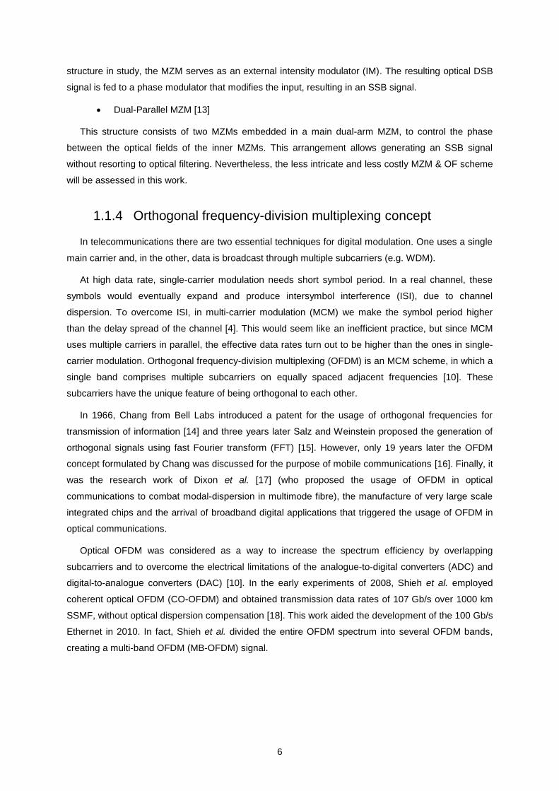
In a network with MB-OFDM technology, the routing is done in the optical domain with the use of
reconfigurable OADMs (ROADMs) and very selective OFs [19]. Figure 1.4 illustrates an example of
the add-drop function, where the optical MB-OFDM signal with bands A, B and C enters an add-drop
node and the optical MB-OFDM signal with bands A, D and C exits, without O/E or E/O conversions
have been done. The red arrow represents the drop function, whereas the green arrow represents the
add function. For obvious reasons, the band D can only be aggregated after the disaggregation of
band B has been performed.
Figure 1.4: Example of the band routing in an add-drop node.
The “Metro Networks Based on Multi-Band Orthogonal Frequency-Division Multiplexing Signals”
(MORFEUS) project proposed the use of MB-OFDM signals in metro networks. This project transmits
virtual carrier-assisted 42.8 Gb/s MB-OFDM signals and evaluates the system performance when
using 2, 3 or 4 bands. Alves et al. have shown that a required optical signal-to-noise ratio (OSNR) of
24 dB for a bit error rate (BER) of 10-3
is required in a 240 km metro ring [20].
After this scope of the work, we can conclude that metro-access networks will benefit from using
MB-OFDM signals.

8
1.2 Motivation
In the new metro-access integrated networks, engineers plan to move all the active components to
the edges of the network [9]. Besides, longer optical paths and higher data rates, than regular
metropolitan networks, are also planned for the near future [9]. Accordingly, cost-effective solutions for
the next-generation optical networks need to be assessed. Next, the motivation for the selection of
technologies and techniques in this work are presented.
The advantages of using OFDM in radio frequency (RF) communication systems are widely known.
Nowadays, OFDM is used in optical communication systems as a technique to increase data rates
with minor distortions on the signal. The use of optical MB-OFDM signals enables routing with
granularity at the sub-wavelength level and provides flexibility on capacity allocation to the next-
generation optical networks [20].
For high data rate, as the bit durations become smaller, the frequency chirp imposed by direct
modulation becomes more severe. Therefore, an external modulator is chosen as a better option. The
MZM is a commonly preferred component for external modulation, providing a high-speed intensity
modulation at broad bandwidth, with low driving voltage and absence of chirp.
To overcome power fading, due to the dispersive transmission of the DSB signal, some techniques
have been proposed, mostly implementing an SSB signal generator. This work uses a simple solution
(i.e. one OF) to supress one sideband of the spectrum.
Telecommunication operators are very rigorous in the planning of a network. Capital and
operational costs need to be reduced, without compromising the system performance. With this
dissertation, we intend to evaluate the performance of this cheap scheme (i.e. MZM & OF) in a metro-
access network, employing virtual carrier-assisted MB-OFDM signals. The following questions arise:
How does this scheme behave within the metro-access integrated networks?
What are the main impairments induced by this off-the-shelf SSB generator?
What are the optimum parameters for the components of this solution which maximise the
performance of the ultra-dense MB-OFDM system?
What is the maximum reach and number of users to whom this system can guarantee a
band capacity of 10 Gb/s?
These questions are the main motivational topics to address and will be fully scrutinized along this
dissertation.
1.3 Objectives and structure of the dissertation
The purpose of this dissertation is to study and characterize a 10 Gb/s per user ultra-dense MB-
OFDM network, employing an off-the-shelf SSB generator. In order to fulfil it, a set of objectives are
proposed:
9
Study and characterisation of the MB-OFDM signals, in the time and frequency domain;
Study and characterisation of the MB-OFDM metro-access integrated network;
Study and characterisation of the performance degradation induced by the SSB signal
generator, based on a single-arm chirpless MZM followed by an OF, in an MB-OFDM
metro-access downstream link that provides 10 Gb/s per user;
Optimization of the MZM bias point and modulation index (MI) and OF features, in order to
maximise the performance of the MB-OFDM integrated network.
To accomplish these objectives, this dissertation is divided in 5 chapters and 2 appendices.
In chapter 2, we start by reviewing the OFDM signal and architecture of the OFDM transmitter and
receiver. Still in this chapter, the virtual carrier-assisted SSB MB-OFDM signal is presented, followed
by the digital signal processing (DSP) algorithm to mitigate the signal-signal beat interference (SSBI).
Also, the downstream of a metro-access integrated network structure is described.
In chapter 3, it is studied the MB-OFDM system and its performance in order to optimize the
numerical parameters of the system, namely the bandwidth of the signal, modulation scheme, MZM
bias point and MI, -3 dB bandwidth of the band selector (BS) and length of the metro network.
Chapter 4 presents the optimization of the OF used to produce the SSB signal, where two filters
are studied: (i) the 2nd
order super-Gaussian (SG); and (ii) the 4th order SG. The power budget of the
access network is firstly assessed using rectangular filters, and then using the optimized SG filters.
The maximum length of the metro-access network and maximum number of users is evaluated.
Chapter 5 reports the final conclusions and the proposals for future work on the subject of this
dissertation.
Appendix A presents some information concerning the transfer function of the single-tap equalizer
used in the OFDM receiver, as well as concerning the thermal and optical noise generated by the
front-end receiver and the OAs in the network, respectively.
In appendix B, the methods used to evaluate the performance of the MB-OFDM system are
presented.
1.4 Main original contributions
The principal original contributions, during the development of this work, are:
The implementation of a simulated metro-access MB-OFDM integrated network, using the
software MATLAB®, for the assessment of the performance of the MB-OFDM signal using
the off-the-shelf SSB generator;
The optimization of the 10 Gb/s signal and equipment used in the system, particularly the
features of the MZM and OF used to generate the SSB signal;

10
Analysis of the power budget of the access network, as well as the maximum length and
number of users in the metro-access network.

11
Chapter 2
Description of the MB-OFDM
system
Description of the MB-OFDM system 2
In this chapter, the OFDM signal used in this work, as well as the MB-OFDM system employed to
transmit and receive multiple OFDM bands, are detailed.

12
2.1 OFDM signal basics
2.1.1 Mathematical formulation of an MCM signal
An MCM signal s(t) is represented as:
1
,0
scN
k i k Si k
s t c s t iT
(2.1)
where t represents the time, ck,i is the i-th information symbol at the k-th subcarrier, Nsc is the number
of subcarriers and TS is the symbol period. Also, sk is the waveform for the k-th subcarrier and is
characterized by:
2 kj f tks t t e
(2.2)
with fk being the frequency of the k-th subcarrier and t being the pulse shaping function:
01,
00,
S
S
t Tt
t t T
(2.3)
From equation (2.1), we conclude that the transmitter requires a collection of Nsc oscillators and
filters to modulate the information symbols in each signal.
2.1.2 Discrete Fourier transform
One of the disadvantages of MCM is the bandwidth requirements in the design of the filters and
oscillators at both transmitter and receiver ends. This bandwidth has to be multiple times larger than
the symbol rate, because conventional MCM uses non-overlapped band-limited signals [10]. By
overlapping the subcarriers in OFDM, the spectral efficiency is increased and this disadvantage is
cancelled. The correlation between any two subcarriers can be defined in terms of the inner product
as:
2*
0 0
sin1 1,
S S
i j i j S
T Ti j Sj f f t j f f T
i j i jS S i j S
f f Ts s s s dt e dt e
T T f f T
(2.4)
where sj* is the complex conjugate of sj. It can be seen that, if subcarriers are apart by:
1
,sc i jS
f f f m mT
(2.5)
then the two subcarriers are orthogonal and do not interfere with each other, i.e.:
1,
,0,
i j
i js s
i j
(2.6)
It were Weinstein and Salz who reported that OFDM modulation/demodulation could be obtained
13
using inverse discrete Fourier transform (IDFT)/discrete Fourier transform (DFT) [15]. Some years
later, a digital algorithm using the inverse fast Fourier transform (IFFT)/FFT was developed to
implement the IDFT/DFT and verified to be very efficient in terms of computation time. This
manipulation avoids the great number of oscillators and filters for modulation and reduces the number
of multiplications needed to modulate/demodulate the OFDM signal, from 2scN to 2log
2
scsc
NN , which
scales almost linearly with the number of subcarriers [10].
Taking into account only one symbol in equation (2.1) and considering equation (2.5) for the best
spectral efficiency (i.e. m = 1), the frequency for the k-th subcarrier is:
kS
kf
T (2.7)
When sampling s(t) every S
sc
T
N, we get n-th sample of the signal:
1 2
0
IDFTsc
sc
knN j
kN
kk
s n c e c (2.8)
At each discrete time [0, 1]scn N , the transmitted signal in equation (2.8) becomes equal to an
Nsc-point IDFT of the information symbol ck, i.e. if we apply the FFT algorithm at the signal in the
receiver, we get the information symbol ck sampled in time-domain.
2.1.3 Cyclic prefix
Whenever a signal travels through a dispersive channel, its subcarriers may express different
group velocity, causing delay td between each other, losing synchronization with the FFT demodulation
window at the receiver and experiencing different central frequencies. The consequence is the
absence of complete symbols and loss of the orthogonality condition [10]. In metro-access networks,
with distances of dozens of kilometres, this is mainly due to CD. The delay spread can be estimated
resorting to the CD parameter at nominal wavelength 0 , 0
D , half-power spectral width of the optical
signal, S and the fibre distance, L, as [2]:
0d St D L (2.9)
where S is [2]:
20
S OFDMBc
(2.10)
with c being the speed of light in vacuum given by 3×10⁸ m/s and BOFDM being the width of the OFDM
band.
When a stream of OFDM symbols is transmitted, a guard interval comprising a number of samples
14
from the end of the symbol is added at the start of each symbol, to resolve ISI due to channel
dispersion. These samples are called cyclic prefix (CP) and its duration must follow the condition:
g dT t (2.11)
That is to say that as long as the delay spread induced by the channel does not exceed the
duration of CP, Tg, it is possible to recover the whole OFDM data. This technique reduces the data
rate, but introduces redundancy and eliminates ISI [4].
The period length of the symbol increases from TS to:
t S gT T T (2.12)
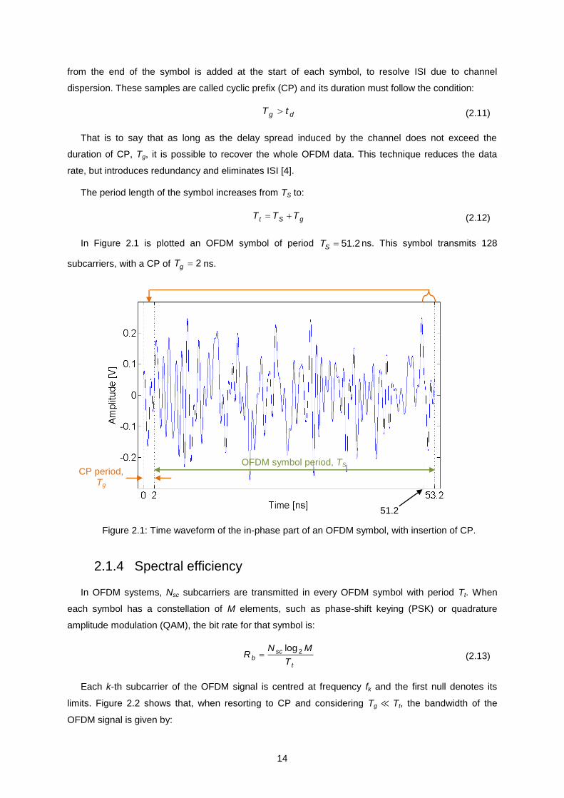
In Figure 2.1 is plotted an OFDM symbol of period 51.2ST ns. This symbol transmits 128
subcarriers, with a CP of 2gT ns.
Figure 2.1: Time waveform of the in-phase part of an OFDM symbol, with insertion of CP.
2.1.4 Spectral efficiency
In OFDM systems, Nsc subcarriers are transmitted in every OFDM symbol with period Tt. When
each symbol has a constellation of M elements, such as phase-shift keying (PSK) or quadrature
amplitude modulation (QAM), the bit rate for that symbol is:
2logsc
bt
N MR
T (2.13)
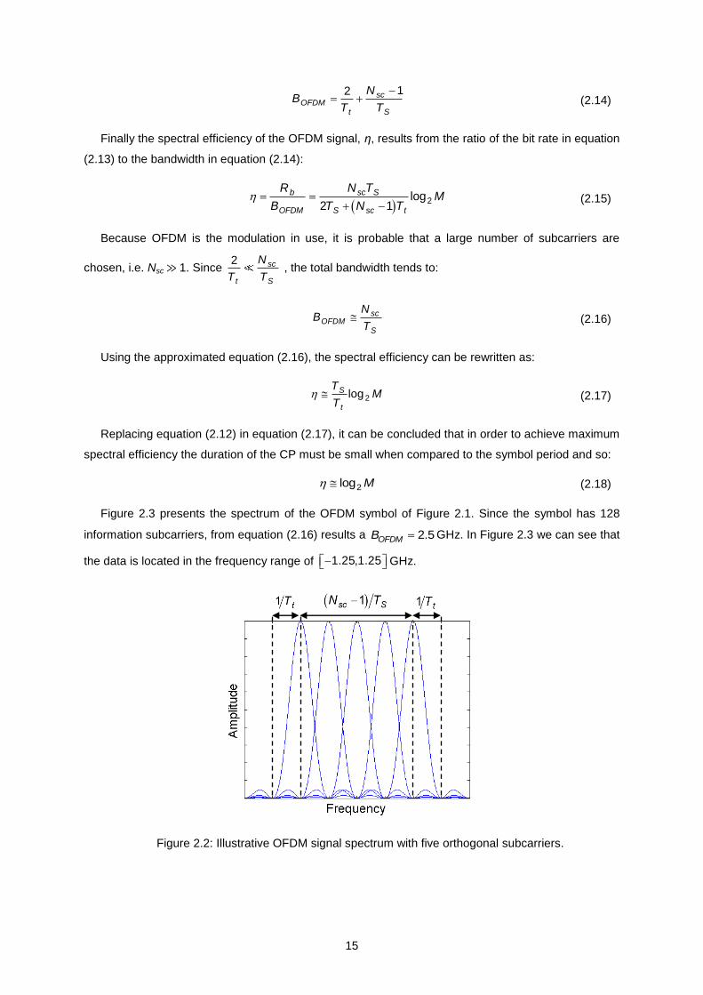
Each k-th subcarrier of the OFDM signal is centred at frequency fk and the first null denotes its
limits. Figure 2.2 shows that, when resorting to CP and considering Tg ≪ Tt, the bandwidth of the
OFDM signal is given by:
OFDM symbol period, TS CP period,
Tg
51.2
15
12 sc
OFDMt S
NB
T T
(2.14)
Finally the spectral efficiency of the OFDM signal, η, results from the ratio of the bit rate in equation
(2.13) to the bandwidth in equation (2.14):
2log
2 1
b sc S
OFDM S sc t
R N TM
B T N T
(2.15)
Because OFDM is the modulation in use, it is probable that a large number of subcarriers are
chosen, i.e. Nsc ≫ 1. Since 2 sc
t S
N
T T , the total bandwidth tends to:
sc
OFDMS
NB
T (2.16)
Using the approximated equation (2.16), the spectral efficiency can be rewritten as:
2logS
t
TM
T (2.17)
Replacing equation (2.12) in equation (2.17), it can be concluded that in order to achieve maximum
spectral efficiency the duration of the CP must be small when compared to the symbol period and so:
2log M (2.18)
Figure 2.3 presents the spectrum of the OFDM symbol of Figure 2.1. Since the symbol has 128
information subcarriers, from equation (2.16) results a 2.5OFDMB GHz. In Figure 2.3 we can see that
the data is located in the frequency range of 1.25,1.25 GHz.
Figure 2.2: Illustrative OFDM signal spectrum with five orthogonal subcarriers.
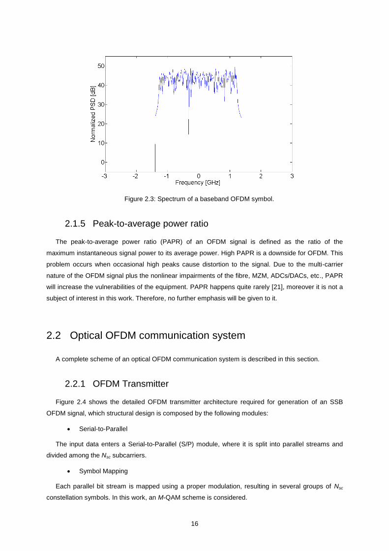
16
Figure 2.3: Spectrum of a baseband OFDM symbol.
2.1.5 Peak-to-average power ratio
The peak-to-average power ratio (PAPR) of an OFDM signal is defined as the ratio of the
maximum instantaneous signal power to its average power. High PAPR is a downside for OFDM. This
problem occurs when occasional high peaks cause distortion to the signal. Due to the multi-carrier
nature of the OFDM signal plus the nonlinear impairments of the fibre, MZM, ADCs/DACs, etc., PAPR
will increase the vulnerabilities of the equipment. PAPR happens quite rarely [21], moreover it is not a
subject of interest in this work. Therefore, no further emphasis will be given to it.
2.2 Optical OFDM communication system
A complete scheme of an optical OFDM communication system is described in this section.
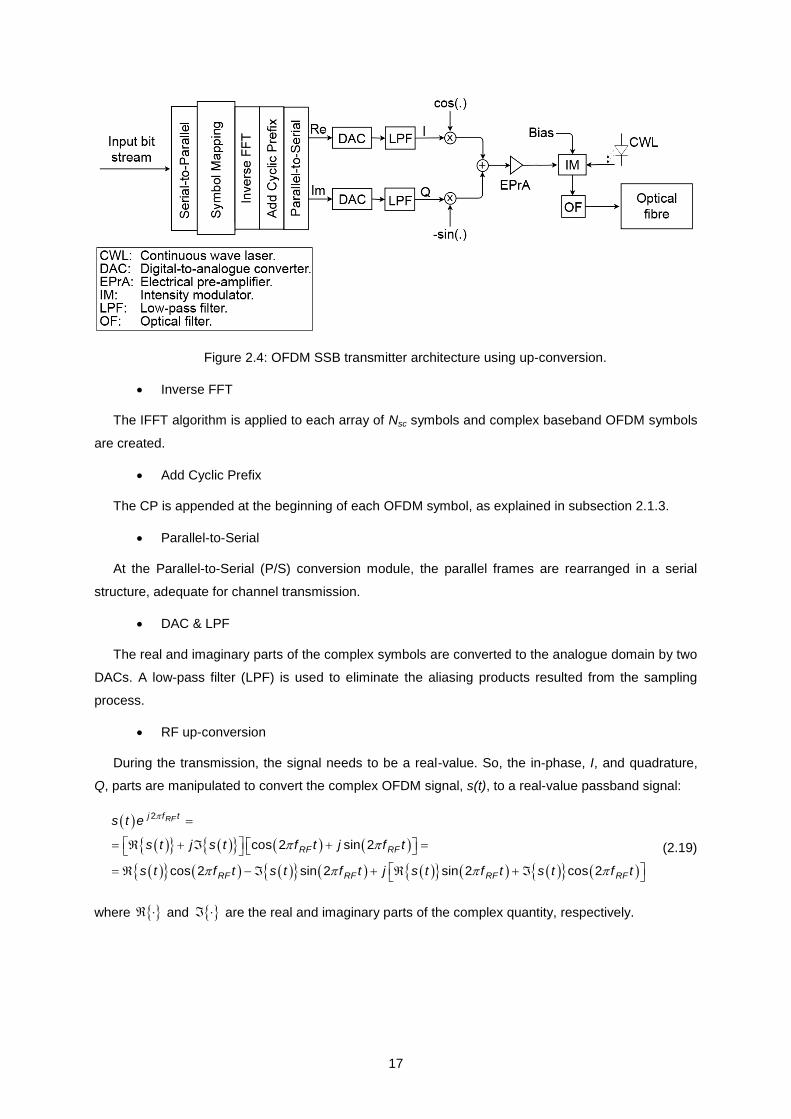
2.2.1 OFDM Transmitter
Figure 2.4 shows the detailed OFDM transmitter architecture required for generation of an SSB
OFDM signal, which structural design is composed by the following modules:
Serial-to-Parallel
The input data enters a Serial-to-Parallel (S/P) module, where it is split into parallel streams and
divided among the Nsc subcarriers.
Symbol Mapping
Each parallel bit stream is mapped using a proper modulation, resulting in several groups of Nsc
constellation symbols. In this work, an M-QAM scheme is considered.
17
Figure 2.4: OFDM SSB transmitter architecture using up-conversion.
Inverse FFT
The IFFT algorithm is applied to each array of Nsc symbols and complex baseband OFDM symbols
are created.
Add Cyclic Prefix
The CP is appended at the beginning of each OFDM symbol, as explained in subsection 2.1.3.
Parallel-to-Serial
At the Parallel-to-Serial (P/S) conversion module, the parallel frames are rearranged in a serial
structure, adequate for channel transmission.
DAC & LPF
The real and imaginary parts of the complex symbols are converted to the analogue domain by two
DACs. A low-pass filter (LPF) is used to eliminate the aliasing products resulted from the sampling
process.
RF up-conversion
During the transmission, the signal needs to be a real-value. So, the in-phase, I, and quadrature,
Q, parts are manipulated to convert the complex OFDM signal, s(t), to a real-value passband signal:
2
cos 2 sin 2
cos 2 sin 2 sin 2 cos 2
RFj f t
RF RF
RF RF RF RF
s t e
s t j s t f t j f t
s t f t s t f t j s t f t s t f t
(2.19)
where and are the real and imaginary parts of the complex quantity, respectively.
18
From equation (2.19), we get a real and imaginary part. If the former is picked, we get the
passband signal sRF(t), at intermediate frequency fRF:
2cos 2 sin 2 RFj f t
RF RF RFs t f t s t f t s t e s t (2.20)
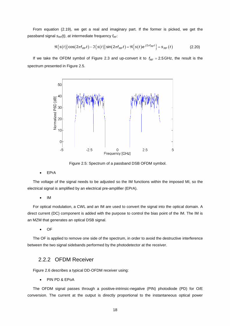
If we take the OFDM symbol of Figure 2.3 and up-convert it to 2.5RFf GHz, the result is the
spectrum presented in Figure 2.5.
Figure 2.5: Spectrum of a passband DSB OFDM symbol.
EPrA
The voltage of the signal needs to be adjusted so the IM functions within the imposed MI, so the
electrical signal is amplified by an electrical pre-amplifier (EPrA).
IM
For optical modulation, a CWL and an IM are used to convert the signal into the optical domain. A
direct current (DC) component is added with the purpose to control the bias point of the IM. The IM is
an MZM that generates an optical DSB signal.
OF
The OF is applied to remove one side of the spectrum, in order to avoid the destructive interference
between the two signal sidebands performed by the photodetector at the receiver.
2.2.2 OFDM Receiver
Figure 2.6 describes a typical DD-OFDM receiver using:
PIN PD & EPoA
The OFDM signal passes through a positive-intrinsic-negative (PIN) photodiode (PD) for O/E
conversion. The current at the output is directly proportional to the instantaneous optical power
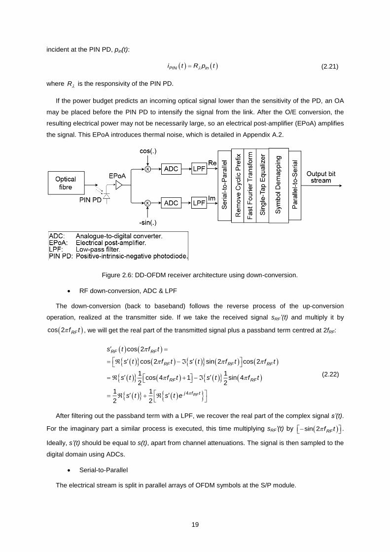
19
incident at the PIN PD, pin(t):
PIN ini t R p t (2.21)
where R is the responsivity of the PIN PD.
If the power budget predicts an incoming optical signal lower than the sensitivity of the PD, an OA
may be placed before the PIN PD to intensify the signal from the link. After the O/E conversion, the
resulting electrical power may not be necessarily large, so an electrical post-amplifier (EPoA) amplifies
the signal. This EPoA introduces thermal noise, which is detailed in Appendix A.2.
Figure 2.6: DD-OFDM receiver architecture using down-conversion.
RF down-conversion, ADC & LPF
The down-conversion (back to baseband) follows the reverse process of the up-conversion
operation, realized at the transmitter side. If we take the received signal sRF’(t) and multiply it by
cos 2 RFf t , we will get the real part of the transmitted signal plus a passband term centred at 2fRF:
4
cos 2
cos 2 sin 2 cos 2
1 1cos 4 1 sin 4
2 2
1 1
2 2RF
RF RF
RF RF RF
RF RF
j f t
s t f t
s t f t s t f t f t
s t f t s t f t
s t s t e
(2.22)
After filtering out the passband term with a LPF, we recover the real part of the complex signal s’(t).
For the imaginary part a similar process is executed, this time multiplying sRF’(t) by sin 2 RFf t .
Ideally, s’(t) should be equal to s(t), apart from channel attenuations. The signal is then sampled to the
digital domain using ADCs.
Serial-to-Parallel
The electrical stream is split in parallel arrays of OFDM symbols at the S/P module.
20
Remove Cyclic Prefix
The CP is removed from the beginning of the symbols.
Fast Fourier Transform
The OFDM symbols enter the FFT module, where they are demodulated, resulting in groups of Nsc
complex symbols.
Single-Tap Equalizer
The distortion induced by the channel is corrected in the single-tap equalizer, detailed in Appendix
A.1. This equalizer has a transfer function that estimates the link properties, which is obtained from the
information provided by the received training symbols. Then, the equalizer compensates for phase
and amplitude errors introduced by the channel in the OFDM symbols.
Symbol Demapping
The subcarriers are demapped and compared to a predetermined constellation scheme in order to
decide upon the received bits.
Parallel-to-Serial
In the end, the signal passes through a final P/S module, before being delivered to the end-user.
Ideally, the output bit stream should be equal to the input one.
2.3 SSB signal generator
2.3.1 Mach-Zehnder modulator
The optical transmitter presented in the previous section makes use of an MZM to modulate the
light. Lithium niobate modulators are designed to maintain low loss and constant switching voltage
over the traditional C and L bands (1530-1610 nm) [22]. These devices have proven to be extremely
reliable [22].
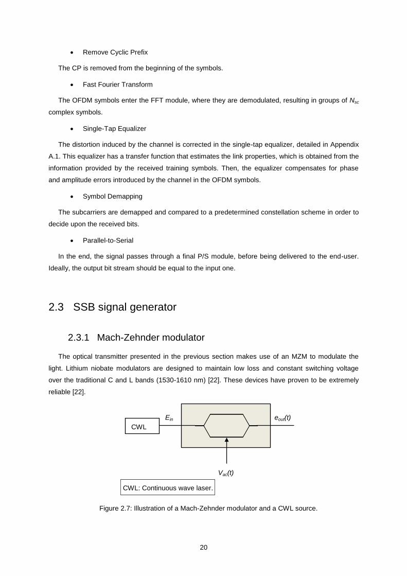
Figure 2.7: Illustration of a Mach-Zehnder modulator and a CWL source.
CWL
Ein eout(t)
Vac(t)
CWL: Continuous wave laser.
21
Figure 2.7 shows a schematic of a single-arm MZM. The chirpless MZM is modelled by the output
optical field oute t , which is a nonlinear function [13]:
cos2
inout ac bias
loss
Ee t v t V
Vi
(2.23)
where inE is the optical field from the CWL output, 1lossi is the optical power insertion loss of the
modulator, acv t is the electrical signal applied to the input and biasV is the modulator bias voltage.
The modulator is characterized by the switching voltage V , which is the voltage required to switch
from a maximum to a minimum of the MZM power transmission characteristic. With neglected insertion
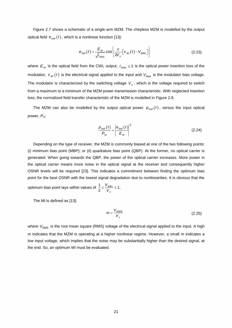
loss, the normalized field transfer characteristic of the MZM is modelled in Figure 2.8.
The MZM can also be modelled by the output optical power outp t , versus the input optical
power, Pin:
2
out out
in in
p t e t
P E (2.24)
Depending on the type of receiver, the MZM is commonly biased at one of the two following points:
(i) minimum bias point (MBP); or (ii) quadrature bias point (QBP). At the former, no optical carrier is
generated. When going towards the QBP, the power of the optical carrier increases. More power in
the optical carrier means more noise in the optical signal at the receiver and consequently higher
OSNR levels will be required [23]. This indicates a commitment between finding the optimum bias
point for the best OSNR with the lowest signal degradation due to nonlinearities. It is obvious that the
optimum bias point lays within values of 1
12
biasV
V
.
The MI is defined as [13]:
RMSV
mV
(2.25)
where RMSV is the root mean square (RMS) voltage of the electrical signal applied to the input. A high
m indicates that the MZM is operating at a higher nonlinear regime. However, a small m indicates a
low input voltage, which implies that the noise may be substantially higher than the desired signal, at
the end. So, an optimum MI must be evaluated.
22
Figure 2.8: Field transfer characteristic of the MZM, with Vπ = 5 V.
2.3.2 Single sideband-optical filter
A passband OF is applied to supress one side of the signal spectrum [4]. Hereinafter, this filter will
be referred to as single sideband-optical filter (SSB-OF). Its bandwidth and selectivity are the main
features to be considered. The selectivity of any filter is the ratio of the -3 dB bandwidth to the
bandwidth at -20 dB and the ideal selectivity happens when Sf = 1:
3
20
dBf
dB
BS
B
(2.26)
The SSB-OF will be adjusted to have such an amplitude response that blocks every frequency
component except for the upper sideband, as seen in Figure 1.3 (b). It should present a very flat
passband, so the output signal power is constant throughout the desired sideband, and sharp cut-offs,
to isolate the upper from the lower sideband.
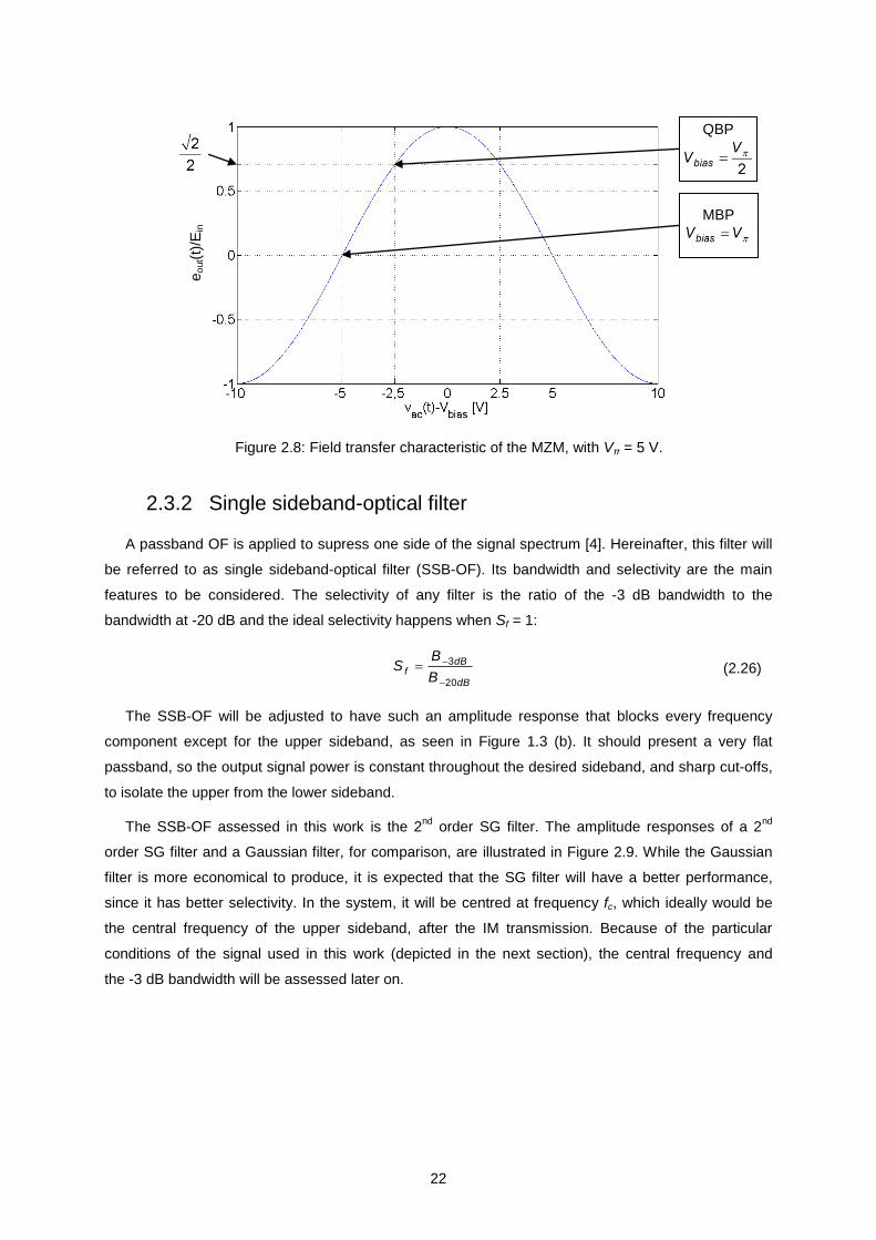
The SSB-OF assessed in this work is the 2nd
order SG filter. The amplitude responses of a 2nd
order SG filter and a Gaussian filter, for comparison, are illustrated in Figure 2.9. While the Gaussian
filter is more economical to produce, it is expected that the SG filter will have a better performance,
since it has better selectivity. In the system, it will be centred at frequency fc, which ideally would be
the central frequency of the upper sideband, after the IM transmission. Because of the particular
conditions of the signal used in this work (depicted in the next section), the central frequency and
the -3 dB bandwidth will be assessed later on.
QBP
MBP
eo
ut(t)
/Ein
23
Figure 2.9: Amplitude response of (a) Gaussian filter and (b) 2nd order SG filter.
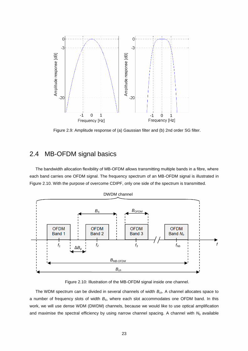
2.4 MB-OFDM signal basics
The bandwidth allocation flexibility of MB-OFDM allows transmitting multiple bands in a fibre, where
each band carries one OFDM signal. The frequency spectrum of an MB-OFDM signal is illustrated in
Figure 2.10. With the purpose of overcome CDIPF, only one side of the spectrum is transmitted.
Figure 2.10: Illustration of the MB-OFDM signal inside one channel.
The WDM spectrum can be divided in several channels of width Bch. A channel allocates space to
a number of frequency slots of width BS, where each slot accommodates one OFDM band. In this
work, we will use dense WDM (DWDM) channels, because we would like to use optical amplification
and maximise the spectral efficiency by using narrow channel spacing. A channel with Nb available
-1 0 1 -1 0 1
DWDM channel
BS BOFDM
BMB-OFDM
Bch
ΔBg
f1 f2 f3 fNb f
24
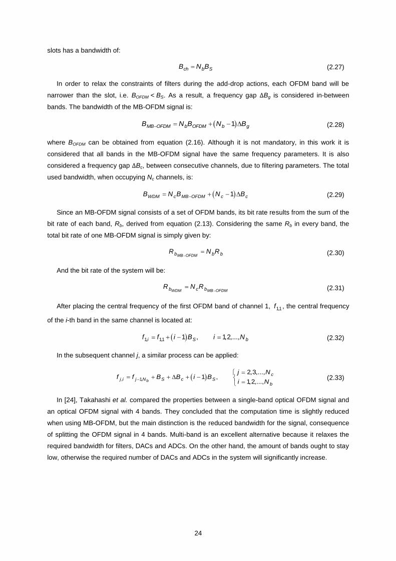
slots has a bandwidth of:
ch b SB N B (2.27)
In order to relax the constraints of filters during the add-drop actions, each OFDM band will be
narrower than the slot, i.e. BOFDM < BS. As a result, a frequency gap ∆Bg is considered in-between
bands. The bandwidth of the MB-OFDM signal is:
1MB OFDM b OFDM b gB N B N B (2.28)
where BOFDM can be obtained from equation (2.16). Although it is not mandatory, in this work it is
considered that all bands in the MB-OFDM signal have the same frequency parameters. It is also
considered a frequency gap ∆Bc, between consecutive channels, due to filtering parameters. The total
used bandwidth, when occupying Nc channels, is:
1WDM c MB OFDM c cB N B N B (2.29)
Since an MB-OFDM signal consists of a set of OFDM bands, its bit rate results from the sum of the
bit rate of each band, Rb, derived from equation (2.13). Considering the same Rb in every band, the
total bit rate of one MB-OFDM signal is simply given by:
MB OFDMb b bR N R
(2.30)
And the bit rate of the system will be:
WDM MB OFDMb c bR N R
(2.31)
After placing the central frequency of the first OFDM band of channel 1, 1,1f , the central frequency
of the i-th band in the same channel is located at:
1, 1,1 1 , 1,2,...,i S bf f i B i N (2.32)
In the subsequent channel j, a similar process can be applied:
, 1,
2,3,...,1 ,
1,2,...,b
cj i j N S c S
b
j Nf f B B i B
i N (2.33)
In [24], Takahashi et al. compared the properties between a single-band optical OFDM signal and
an optical OFDM signal with 4 bands. They concluded that the computation time is slightly reduced
when using MB-OFDM, but the main distinction is the reduced bandwidth for the signal, consequence
of splitting the OFDM signal in 4 bands. Multi-band is an excellent alternative because it relaxes the
required bandwidth for filters, DACs and ADCs. On the other hand, the amount of bands ought to stay
low, otherwise the required number of DACs and ADCs in the system will significantly increase.
25
2.5 Virtual carrier-assisted MB-OFDM signal
At a DD receiver, the optical carrier is used to assist the photodetection at the PIN PD. Let’s
imagine one OFDM band arriving at the receiver. The PIN PD collects the optical field:
in RFe t A s t (2.34)
where RFs t is the SSB signal and A is the optical carrier generated by the IM. In subsection 2.2.2,
we saw that the PIN PD is modelled as the square law of the absolute value of the received optical
field and by using equations (2.21) and (2.34) we get, apart from the responsivity:
2 22 2PIN in RF RFi t e t A s t A s t (2.35)
with A2 being the DC component of the optical carrier,
2
RFs t being a second-order term resulting
from the SSBI and 2 RFA s t being the resulting beat between the OFDM signal and optical
carrier. Actually, we are only interested in the last term, for it has a replica of the transmitted data
signal. However, depending on the gap between band and optical carrier, the SSBI term will have
greater or less impact in the receiver.
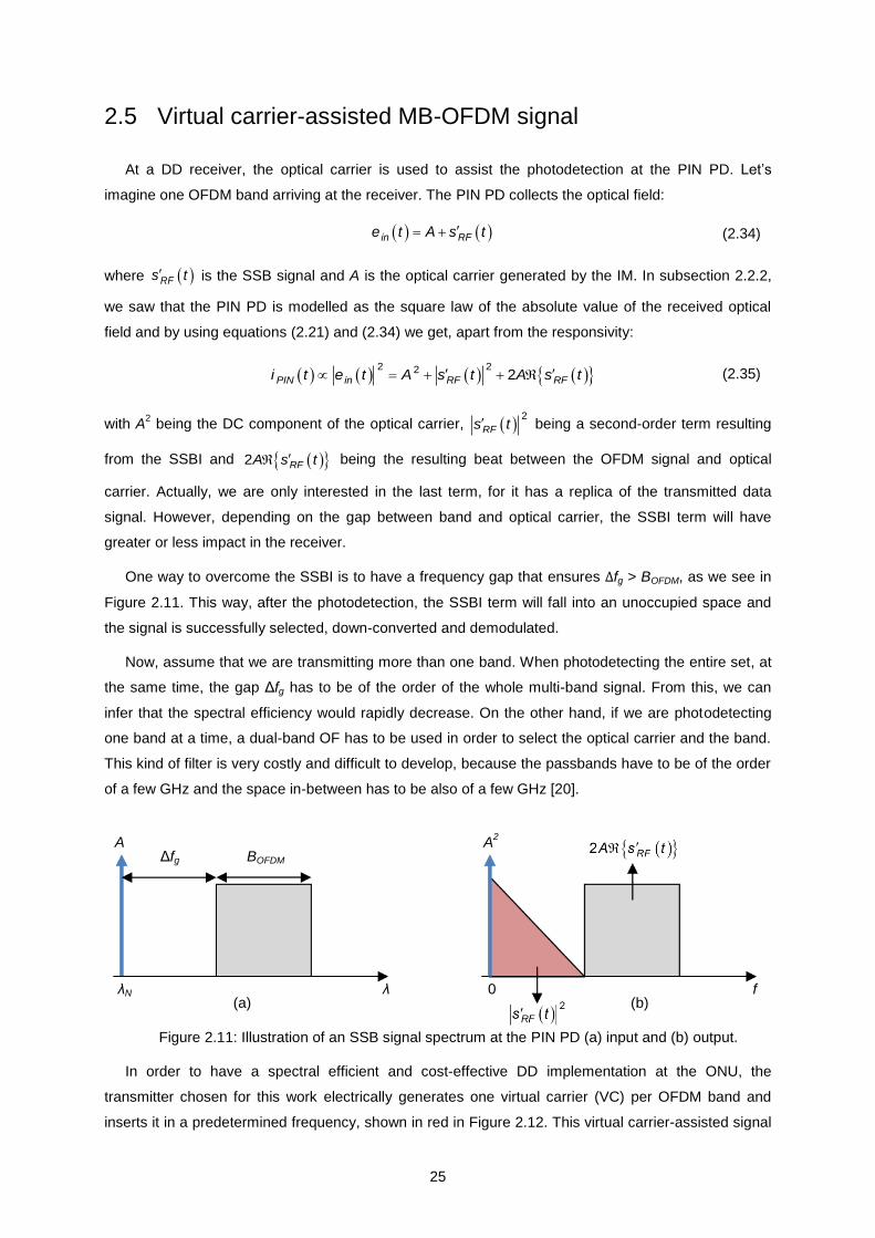
One way to overcome the SSBI is to have a frequency gap that ensures ∆fg > BOFDM, as we see in
Figure 2.11. This way, after the photodetection, the SSBI term will fall into an unoccupied space and
the signal is successfully selected, down-converted and demodulated.
Now, assume that we are transmitting more than one band. When photodetecting the entire set, at
the same time, the gap Δfg has to be of the order of the whole multi-band signal. From this, we can
infer that the spectral efficiency would rapidly decrease. On the other hand, if we are photodetecting
one band at a time, a dual-band OF has to be used in order to select the optical carrier and the band.
This kind of filter is very costly and difficult to develop, because the passbands have to be of the order
of a few GHz and the space in-between has to be also of a few GHz [20].
Figure 2.11: Illustration of an SSB signal spectrum at the PIN PD (a) input and (b) output.
In order to have a spectral efficient and cost-effective DD implementation at the ONU, the
transmitter chosen for this work electrically generates one virtual carrier (VC) per OFDM band and
inserts it in a predetermined frequency, shown in red in Figure 2.12. This virtual carrier-assisted signal
λN λ 0 f
A A2
BOFDM Δfg
(a) (b)
26
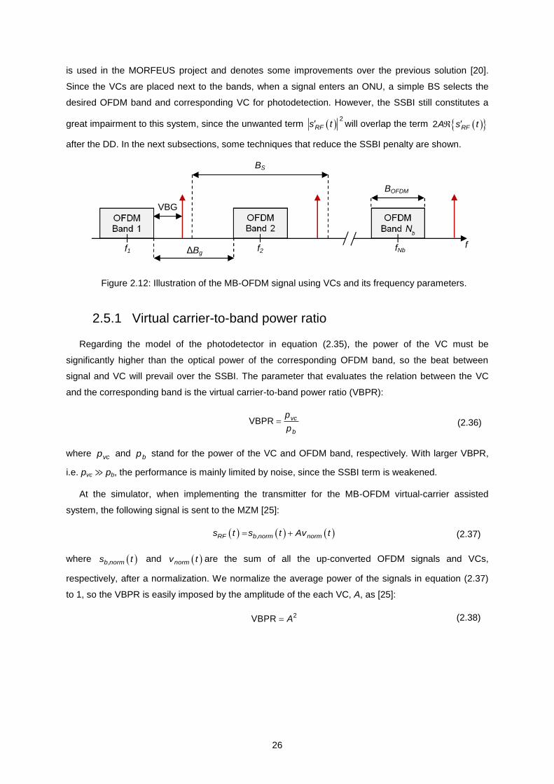
is used in the MORFEUS project and denotes some improvements over the previous solution [20].
Since the VCs are placed next to the bands, when a signal enters an ONU, a simple BS selects the
desired OFDM band and corresponding VC for photodetection. However, the SSBI still constitutes a
great impairment to this system, since the unwanted term 2
RFs t will overlap the term 2 RFA s t
after the DD. In the next subsections, some techniques that reduce the SSBI penalty are shown.
Figure 2.12: Illustration of the MB-OFDM signal using VCs and its frequency parameters.
2.5.1 Virtual carrier-to-band power ratio
Regarding the model of the photodetector in equation (2.35), the power of the VC must be
significantly higher than the optical power of the corresponding OFDM band, so the beat between
signal and VC will prevail over the SSBI. The parameter that evaluates the relation between the VC
and the corresponding band is the virtual carrier-to-band power ratio (VBPR):
VBPR vc
b
p
p (2.36)
where vcp and bp stand for the power of the VC and OFDM band, respectively. With larger VBPR,
i.e. pvc ≫ pb, the performance is mainly limited by noise, since the SSBI term is weakened.
At the simulator, when implementing the transmitter for the MB-OFDM virtual-carrier assisted
system, the following signal is sent to the MZM [25]:
,RF b norm norms t s t Av t (2.37)
where ,b norms t and normv t are the sum of all the up-converted OFDM signals and VCs,
respectively, after a normalization. We normalize the average power of the signals in equation (2.37)
to 1, so the VBPR is easily imposed by the amplitude of the each VC, A, as [25]:
2VBPR A (2.38)
VBG
BS
ΔBg f1 f2 fNb
f
BOFDM
27
2.5.3 Virtual carrier-to-band gap
To have an SSBI-free signal, a frequency gap between the pair band-VC larger than the bandwidth
of the band must be employed, represented in Figure 2.12 as virtual carrier-to-band gap (VBG). BOFDM
has usually a few GHz, consequently VBG must also be of the same order of GHz. We already saw
that this is an undesirable condition.
A tuneable VBG is considered in [26] to help diminishing the SSBI. In that work, Peng et al. found a
normalized gap of 0.35 to be the optimum VBG, chosen to achieve the best trading levels between
SSBI penalty and residual image beat interference (which results from the aliasing products of the
DACs). With an OFDM bandwidth of ~3 GHz, this would require a frequency gap of 1.05 GHz
between the pair band-VC, which is still a large VBG to choose for this work.
To ensure that the VC does not interfere with the signal itself, we resort to the condition:
VBG ,sck f k (2.39)
where Δfsc comes from equation (2.5), considering m = 1. This takes into consideration the fact that all
subcarriers are equally spaced, so the VC will be placed where the nulls of the sinc function occurs
(see Figure 2.2, considering Tt ≅ TS).
Regarding the central frequency of a given slot, ,j if , its corresponding VC will be allocated at:
, , VBG
2j i
OFDMvc j i
Bf f (2.40)
2.5.4 Iterative SSBI mitigation algorithm
In the previous subsection it was concluded that we need a small VBG to have high spectral
efficiency. Doing so, we would have to apply a very high VBPR, to effectively demodulate the signal
with low BER levels. Yet, it was already seen that the noise power is proportional to the VBPR. So, we
resort to DSP algorithms to reduce the impact of SSBI, as Peng et al. demonstrated in [26]. This is an
iterative SSBI cancelation technique, which works in two sequential modes: (i) training mode; and (ii)
data mode. During the former, only training symbols are received and the goal is to get the number of
iterations required to estimate the SSBI term resulting from the square law of the PIN PD. The quality
of the signal is monitored throughout the iterations and this mode runs until the performance meets
certain pre-imposed conditions. Afterwards, in the data mode, the algorithm uses the information
gathered in the previous mode to get a virtually SSBI-free signal.
This technique was studied in detail by Mendes in [27]. The concept of the feedback loop of the
SSBI estimation is depicted in Figure 2.13. In the insets of Figure 2.13 we can see a sketch exhibiting
the frequency spectrum at some stages of the algorithm, demonstrative of the ideal mitigation of the
SSBI in the signal, pictured in red and blue, respectively.
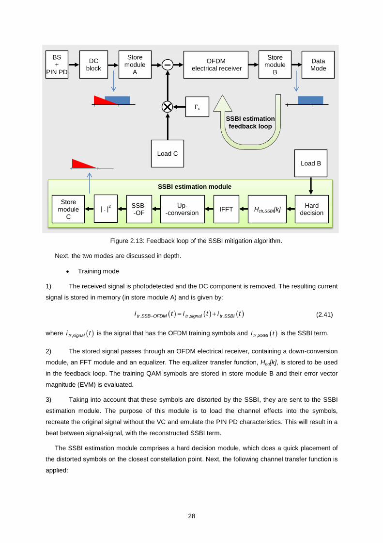
28
Figure 2.13: Feedback loop of the SSBI mitigation algorithm.
Next, the two modes are discussed in depth.
Training mode
1) The received signal is photodetected and the DC component is removed. The resulting current
signal is stored in memory (in store module A) and is given by:
, , ,tr SSB OFDM tr signal tr SSBIi t i t i t (2.41)
where ,tr signali t is the signal that has the OFDM training symbols and ,tr SSBIi t is the SSBI term.
2) The stored signal passes through an OFDM electrical receiver, containing a down-conversion
module, an FFT module and an equalizer. The equalizer transfer function, Heq[k], is stored to be used
in the feedback loop. The training QAM symbols are stored in store module B and their error vector
magnitude (EVM) is evaluated.
3) Taking into account that these symbols are distorted by the SSBI, they are sent to the SSBI
estimation module. The purpose of this module is to load the channel effects into the symbols,
recreate the original signal without the VC and emulate the PIN PD characteristics. This will result in a
beat between signal-signal, with the reconstructed SSBI term.
The SSBI estimation module comprises a hard decision module, which does a quick placement of
the distorted symbols on the closest constellation point. Next, the following channel transfer function is
applied:
BS +
PIN PD
DC block
Store module
A
OFDM electrical receiver
Store module
B
Γc
Load C
Hard decision
Hch,SSBI[k] IFFT SSB- -OF
Up- -conversion
| . |2
Store module
C
Load B
Data Mode
SSBI estimation module
SSBI estimation
feedback loop
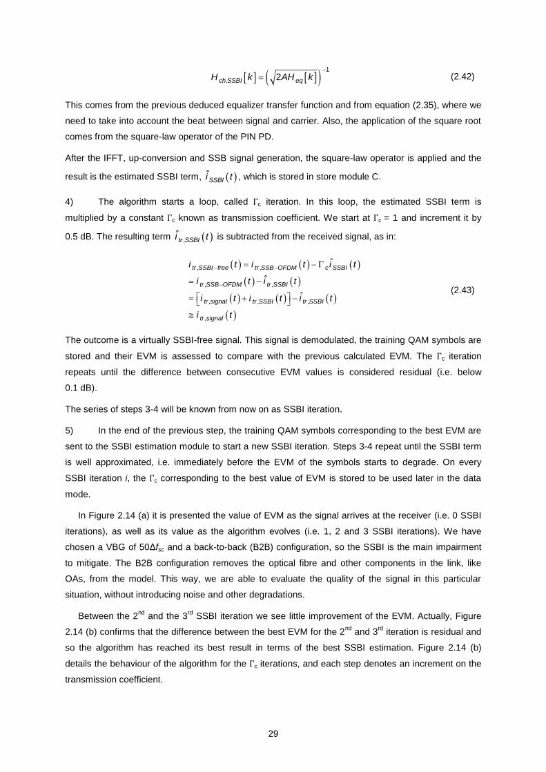
29
1
, 2ch SSBI eqH k AH k (2.42)
This comes from the previous deduced equalizer transfer function and from equation (2.35), where we
need to take into account the beat between signal and carrier. Also, the application of the square root
comes from the square-law operator of the PIN PD.
After the IFFT, up-conversion and SSB signal generation, the square-law operator is applied and the
result is the estimated SSBI term, ˆSSBIi t , which is stored in store module C.
4) The algorithm starts a loop, called Γc iteration. In this loop, the estimated SSBI term is
multiplied by a constant Γc known as transmission coefficient. We start at Γc = 1 and increment it by
0.5 dB. The resulting term ,ˆtr SSBIi t is subtracted from the received signal, as in:
, ,
, ,
, , ,
,
ˆ
ˆ
ˆ
tr SSBI free tr SSB OFDM c SSBI
tr SSB OFDM tr SSBI
tr signal tr SSBI tr SSBI
tr signal
i t i t i t
i t i t
i t i t i t
i t
(2.43)
The outcome is a virtually SSBI-free signal. This signal is demodulated, the training QAM symbols are
stored and their EVM is assessed to compare with the previous calculated EVM. The Γc iteration
repeats until the difference between consecutive EVM values is considered residual (i.e. below
0.1 dB).
The series of steps 3-4 will be known from now on as SSBI iteration.
5) In the end of the previous step, the training QAM symbols corresponding to the best EVM are
sent to the SSBI estimation module to start a new SSBI iteration. Steps 3-4 repeat until the SSBI term
is well approximated, i.e. immediately before the EVM of the symbols starts to degrade. On every
SSBI iteration i, the Γc corresponding to the best value of EVM is stored to be used later in the data
mode.
In Figure 2.14 (a) it is presented the value of EVM as the signal arrives at the receiver (i.e. 0 SSBI
iterations), as well as its value as the algorithm evolves (i.e. 1, 2 and 3 SSBI iterations). We have
chosen a VBG of 50Δfsc and a back-to-back (B2B) configuration, so the SSBI is the main impairment
to mitigate. The B2B configuration removes the optical fibre and other components in the link, like
OAs, from the model. This way, we are able to evaluate the quality of the signal in this particular
situation, without introducing noise and other degradations.
Between the 2nd
and the 3rd
SSBI iteration we see little improvement of the EVM. Actually, Figure
2.14 (b) confirms that the difference between the best EVM for the 2nd
and 3rd
iteration is residual and
so the algorithm has reached its best result in terms of the best SSBI estimation. Figure 2.14 (b)
details the behaviour of the algorithm for the Γc iterations, and each step denotes an increment on the
transmission coefficient.
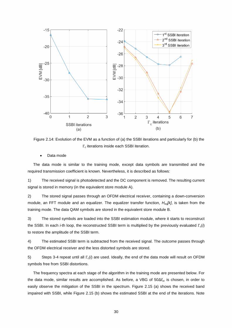
30
Figure 2.14: Evolution of the EVM as a function of (a) the SSBI iterations and particularly for (b) the
Γc iterations inside each SSBI iteration.
Data mode
The data mode is similar to the training mode, except data symbols are transmitted and the
required transmission coefficient is known. Nevertheless, it is described as follows:
1) The received signal is photodetected and the DC component is removed. The resulting current
signal is stored in memory (in the equivalent store module A).
2) The stored signal passes through an OFDM electrical receiver, containing a down-conversion
module, an FFT module and an equalizer. The equalizer transfer function, Heq[k], is taken from the
training mode. The data QAM symbols are stored in the equivalent store module B.
3) The stored symbols are loaded into the SSBI estimation module, where it starts to reconstruct
the SSBI. In each i-th loop, the reconstructed SSBI term is multiplied by the previously evaluated Γc(i)
to restore the amplitude of the SSBI term.
4) The estimated SSBI term is subtracted from the received signal. The outcome passes through
the OFDM electrical receiver and the less distorted symbols are stored.
5) Steps 3-4 repeat until all Γc(i) are used. Ideally, the end of the data mode will result on OFDM
symbols free from SSBI distortions.
The frequency spectra at each stage of the algorithm in the training mode are presented below. For
the data mode, similar results are accomplished. As before, a VBG of 50Δfsc is chosen, in order to
easily observe the mitigation of the SSBI in the spectrum. Figure 2.15 (a) shows the received band
impaired with SSBI, while Figure 2.15 (b) shows the estimated SSBI at the end of the iterations. Note
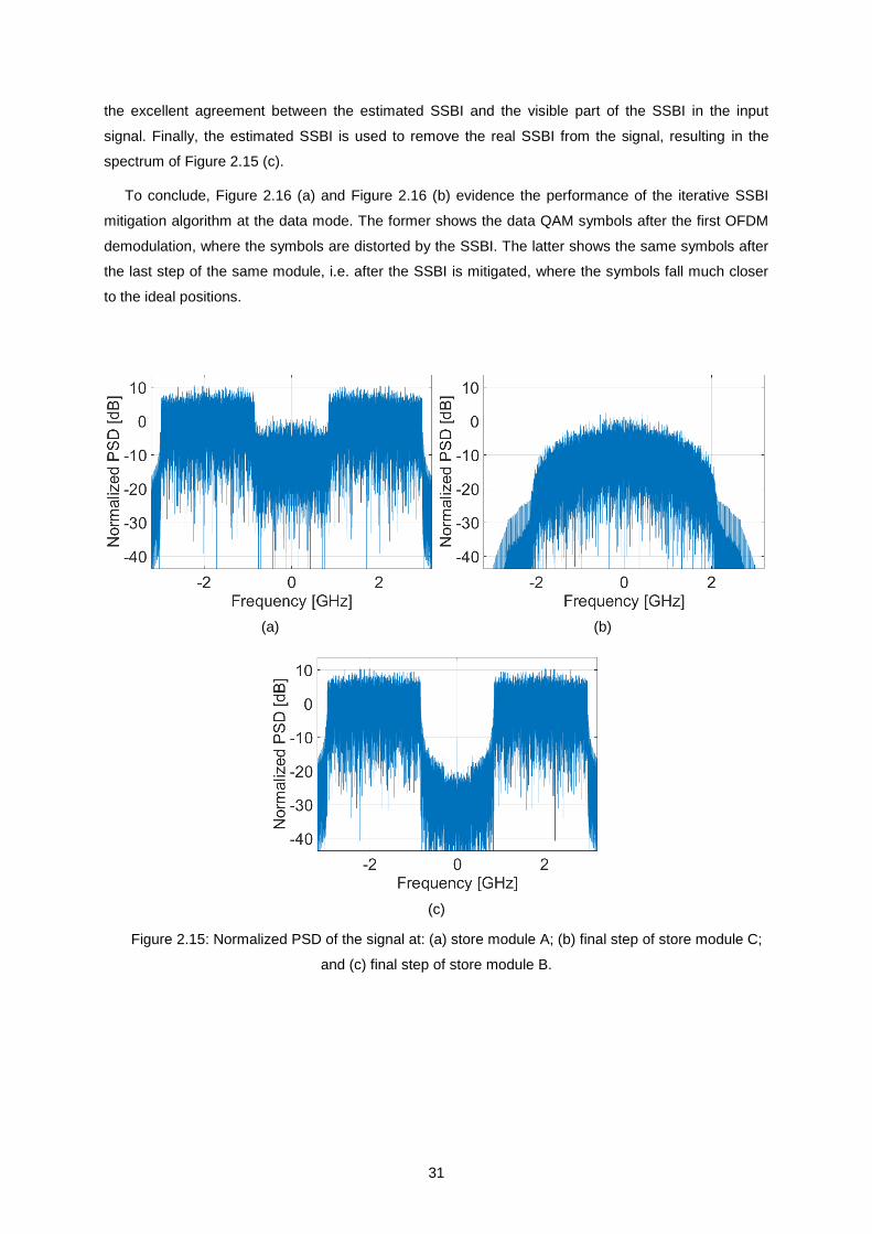
31
the excellent agreement between the estimated SSBI and the visible part of the SSBI in the input
signal. Finally, the estimated SSBI is used to remove the real SSBI from the signal, resulting in the
spectrum of Figure 2.15 (c).
To conclude, Figure 2.16 (a) and Figure 2.16 (b) evidence the performance of the iterative SSBI
mitigation algorithm at the data mode. The former shows the data QAM symbols after the first OFDM
demodulation, where the symbols are distorted by the SSBI. The latter shows the same symbols after
the last step of the same module, i.e. after the SSBI is mitigated, where the symbols fall much closer
to the ideal positions.
(a)
(b)
(c)
Figure 2.15: Normalized PSD of the signal at: (a) store module A; (b) final step of store module C;
and (c) final step of store module B.
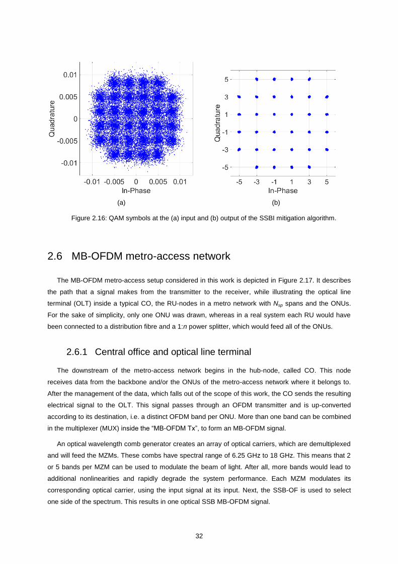
32
(a)
(b)
Figure 2.16: QAM symbols at the (a) input and (b) output of the SSBI mitigation algorithm.
2.6 MB-OFDM metro-access network
The MB-OFDM metro-access setup considered in this work is depicted in Figure 2.17. It describes
the path that a signal makes from the transmitter to the receiver, while illustrating the optical line
terminal (OLT) inside a typical CO, the RU-nodes in a metro network with Nsp spans and the ONUs.
For the sake of simplicity, only one ONU was drawn, whereas in a real system each RU would have
been connected to a distribution fibre and a 1:n power splitter, which would feed all of the ONUs.
2.6.1 Central office and optical line terminal
The downstream of the metro-access network begins in the hub-node, called CO. This node
receives data from the backbone and/or the ONUs of the metro-access network where it belongs to.
After the management of the data, which falls out of the scope of this work, the CO sends the resulting
electrical signal to the OLT. This signal passes through an OFDM transmitter and is up-converted
according to its destination, i.e. a distinct OFDM band per ONU. More than one band can be combined
in the multiplexer (MUX) inside the “MB-OFDM Tx”, to form an MB-OFDM signal.
An optical wavelength comb generator creates an array of optical carriers, which are demultiplexed
and will feed the MZMs. These combs have spectral range of 6.25 GHz to 18 GHz. This means that 2
or 5 bands per MZM can be used to modulate the beam of light. After all, more bands would lead to
additional nonlinearities and rapidly degrade the system performance. Each MZM modulates its
corresponding optical carrier, using the input signal at its input. Next, the SSB-OF is used to select
one side of the spectrum. This results in one optical SSB MB-OFDM signal.
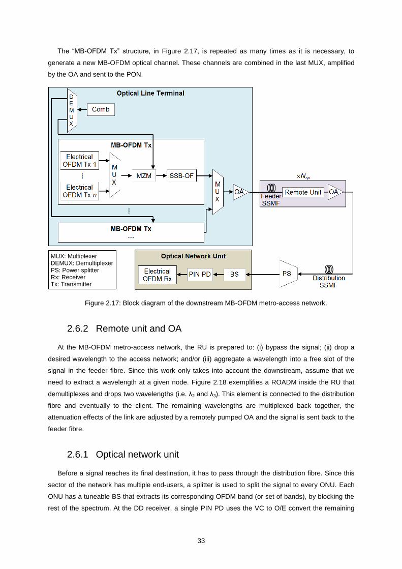
33
The “MB-OFDM Tx” structure, in Figure 2.17, is repeated as many times as it is necessary, to
generate a new MB-OFDM optical channel. These channels are combined in the last MUX, amplified
by the OA and sent to the PON.
Figure 2.17: Block diagram of the downstream MB-OFDM metro-access network.
2.6.2 Remote unit and OA
At the MB-OFDM metro-access network, the RU is prepared to: (i) bypass the signal; (ii) drop a
desired wavelength to the access network; and/or (iii) aggregate a wavelength into a free slot of the
signal in the feeder fibre. Since this work only takes into account the downstream, assume that we
need to extract a wavelength at a given node. Figure 2.18 exemplifies a ROADM inside the RU that
demultiplexes and drops two wavelengths (i.e. λ2 and λ3). This element is connected to the distribution
fibre and eventually to the client. The remaining wavelengths are multiplexed back together, the
attenuation effects of the link are adjusted by a remotely pumped OA and the signal is sent back to the
feeder fibre.
2.6.1 Optical network unit
Before a signal reaches its final destination, it has to pass through the distribution fibre. Since this
sector of the network has multiple end-users, a splitter is used to split the signal to every ONU. Each
ONU has a tuneable BS that extracts its corresponding OFDM band (or set of bands), by blocking the
rest of the spectrum. At the DD receiver, a single PIN PD uses the VC to O/E convert the remaining
MUX: Multiplexer DEMUX: Demultiplexer PS: Power splitter Rx: Receiver Tx: Transmitter
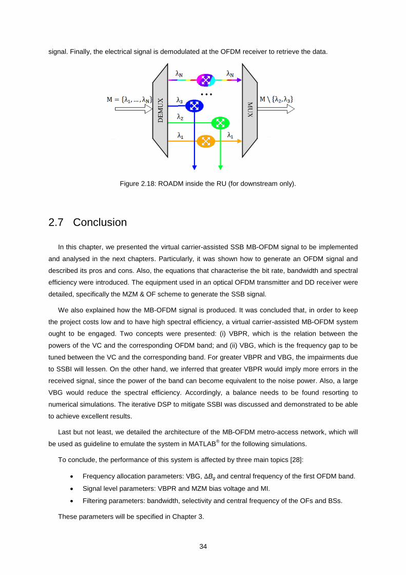
34
signal. Finally, the electrical signal is demodulated at the OFDM receiver to retrieve the data.
Figure 2.18: ROADM inside the RU (for downstream only).
2.7 Conclusion
In this chapter, we presented the virtual carrier-assisted SSB MB-OFDM signal to be implemented
and analysed in the next chapters. Particularly, it was shown how to generate an OFDM signal and
described its pros and cons. Also, the equations that characterise the bit rate, bandwidth and spectral
efficiency were introduced. The equipment used in an optical OFDM transmitter and DD receiver were
detailed, specifically the MZM & OF scheme to generate the SSB signal.
We also explained how the MB-OFDM signal is produced. It was concluded that, in order to keep
the project costs low and to have high spectral efficiency, a virtual carrier-assisted MB-OFDM system
ought to be engaged. Two concepts were presented: (i) VBPR, which is the relation between the
powers of the VC and the corresponding OFDM band; and (ii) VBG, which is the frequency gap to be
tuned between the VC and the corresponding band. For greater VBPR and VBG, the impairments due
to SSBI will lessen. On the other hand, we inferred that greater VBPR would imply more errors in the
received signal, since the power of the band can become equivalent to the noise power. Also, a large
VBG would reduce the spectral efficiency. Accordingly, a balance needs to be found resorting to
numerical simulations. The iterative DSP to mitigate SSBI was discussed and demonstrated to be able
to achieve excellent results.
Last but not least, we detailed the architecture of the MB-OFDM metro-access network, which will
be used as guideline to emulate the system in MATLAB® for the following simulations.
To conclude, the performance of this system is affected by three main topics [28]:
Frequency allocation parameters: VBG, ∆Bg and central frequency of the first OFDM band.
Signal level parameters: VBPR and MZM bias voltage and MI.
Filtering parameters: bandwidth, selectivity and central frequency of the OFs and BSs.
These parameters will be specified in Chapter 3.
35
Chapter 3
Optimization of the parameters of
the MB-OFDM system Optimization of the parameters of the MB-OFDM system 3
In this chapter, we detail and optimize the numerical parameters of the virtual carrier-assisted
MB-OFDM metro-access system, in order to maximise its performance.
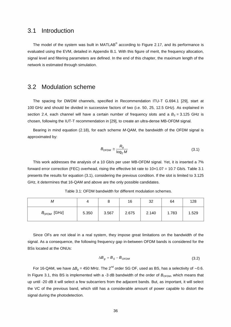
36
3.1 Introduction
The model of the system was built in MATLAB® according to Figure 2.17, and its performance is
evaluated using the EVM, detailed in Appendix B.1. With this figure of merit, the frequency allocation,
signal level and filtering parameters are defined. In the end of this chapter, the maximum length of the
network is estimated through simulation.
3.2 Modulation scheme
The spacing for DWDM channels, specified in Recommendation ITU-T G.694.1 [29], start at
100 GHz and should be divided in successive factors of two (i.e. 50, 25, 12.5 GHz). As explained in
section 2.4, each channel will have a certain number of frequency slots and a BS = 3.125 GHz is
chosen, following the IUT-T recommendation in [29], to create an ultra-dense MB-OFDM signal.
Bearing in mind equation (2.18), for each scheme M-QAM, the bandwidth of the OFDM signal is
approximated by:
2log
bOFDM
RB
M (3.1)
This work addresses the analysis of a 10 Gb/s per user MB-OFDM signal. Yet, it is inserted a 7%
forward error correction (FEC) overhead, rising the effective bit rate to 10×1.07 = 10.7 Gb/s. Table 3.1
presents the results for equation (3.1), considering the previous condition. If the slot is limited to 3.125
GHz, it determines that 16-QAM and above are the only possible candidates.
Table 3.1: OFDM bandwidth for different modulation schemes.
M 4 8 16 32 64 128
OFDMB [GHz] 5.350 3.567 2.675 2.140 1.783 1.529
Since OFs are not ideal in a real system, they impose great limitations on the bandwidth of the
signal. As a consequence, the following frequency gap in-between OFDM bands is considered for the
BSs located at the ONUs:
g S OFDMB B B (3.2)
For 16-QAM, we have ∆Bg = 450 MHz. The 2nd
order SG OF, used as BS, has a selectivity of ~0.6.
In Figure 3.1, this BS is implemented with a -3 dB bandwidth of the order of BOFDM, which means that
up until -20 dB it will select a few subcarriers from the adjacent bands. But, as important, it will select
the VC of the previous band, which still has a considerable amount of power capable to distort the
signal during the photodetection.
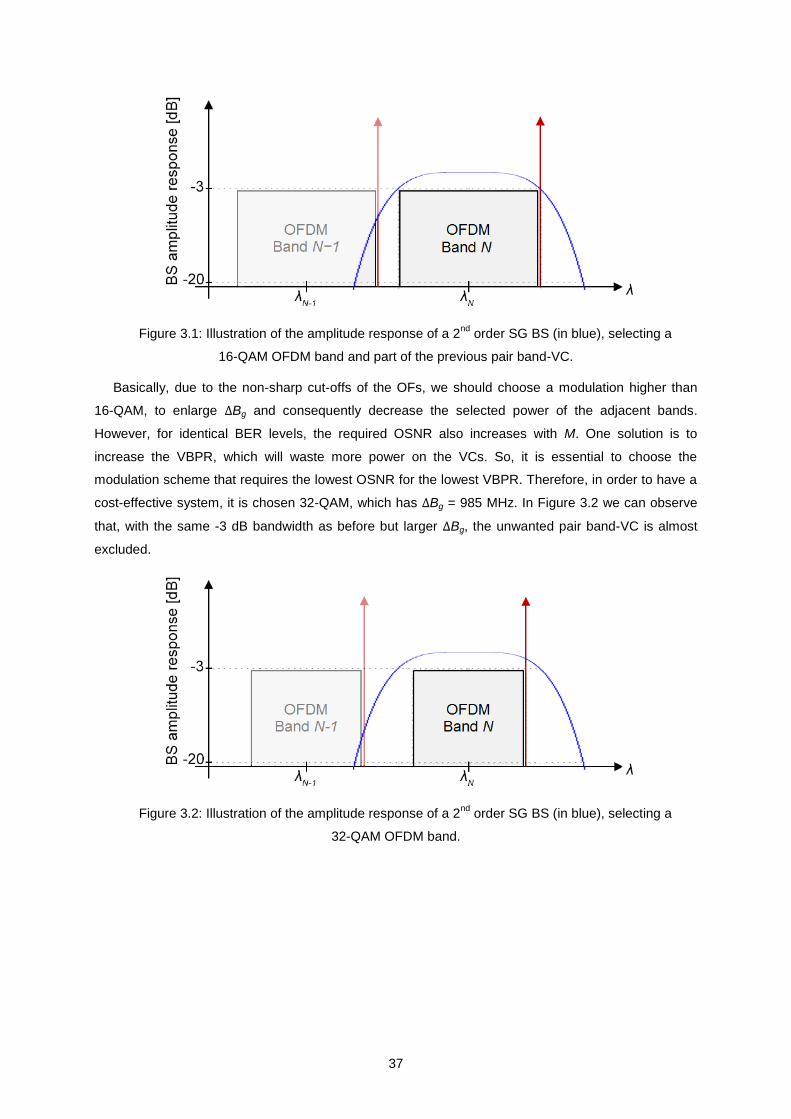
37
Figure 3.1: Illustration of the amplitude response of a 2nd
order SG BS (in blue), selecting a
16-QAM OFDM band and part of the previous pair band-VC.
Basically, due to the non-sharp cut-offs of the OFs, we should choose a modulation higher than
16-QAM, to enlarge ∆Bg and consequently decrease the selected power of the adjacent bands.
However, for identical BER levels, the required OSNR also increases with M. One solution is to
increase the VBPR, which will waste more power on the VCs. So, it is essential to choose the
modulation scheme that requires the lowest OSNR for the lowest VBPR. Therefore, in order to have a
cost-effective system, it is chosen 32-QAM, which has ∆Bg = 985 MHz. In Figure 3.2 we can observe
that, with the same -3 dB bandwidth as before but larger ∆Bg, the unwanted pair band-VC is almost
excluded.
Figure 3.2: Illustration of the amplitude response of a 2nd
order SG BS (in blue), selecting a
32-QAM OFDM band.
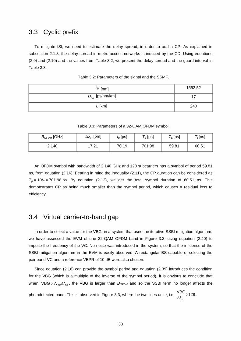
38
3.3 Cyclic prefix
To mitigate ISI, we need to estimate the delay spread, in order to add a CP. As explained in
subsection 2.1.3, the delay spread in metro-access networks is induced by the CD. Using equations
(2.9) and (2.10) and the values from Table 3.2, we present the delay spread and the guard interval in
Table 3.3.
Table 3.2: Parameters of the signal and the SSMF.
0 [nm] 1552.52
0D [ps/nm/km] 17
L [km] 240
Table 3.3: Parameters of a 32-QAM OFDM symbol.
BOFDM [GHz] S [pm] td [ps] Tg [ps] TS [ns] Tt [ns]
2.140 17.21 70.19 701.98 59.81 60.51
An OFDM symbol with bandwidth of 2.140 GHz and 128 subcarriers has a symbol of period 59.81
ns, from equation (2.16). Bearing in mind the inequality (2.11), the CP duration can be considered as
Tg = 10td = 701.98 ps. By equation (2.12), we get the total symbol duration of 60.51 ns. This
demonstrates CP as being much smaller than the symbol period, which causes a residual loss to
efficiency.
3.4 Virtual carrier-to-band gap
In order to select a value for the VBG, in a system that uses the iterative SSBI mitigation algorithm,
we have assessed the EVM of one 32-QAM OFDM band in Figure 3.3, using equation (2.40) to
impose the frequency of the VC. No noise was introduced in the system, so that the influence of the
SSBI mitigation algorithm in the EVM is easily observed. A rectangular BS capable of selecting the
pair band-VC and a reference VBPR of 10 dB were also chosen.
Since equation (2.16) can provide the symbol period and equation (2.39) introduces the condition
for the VBG (which is a multiple of the inverse of the symbol period), it is obvious to conclude that
when VBG sc scN f , the VBG is larger than BOFDM and so the SSBI term no longer affects the
photodetected band. This is observed in Figure 3.3, where the two lines unite, i.e. VBG
>128scf
.
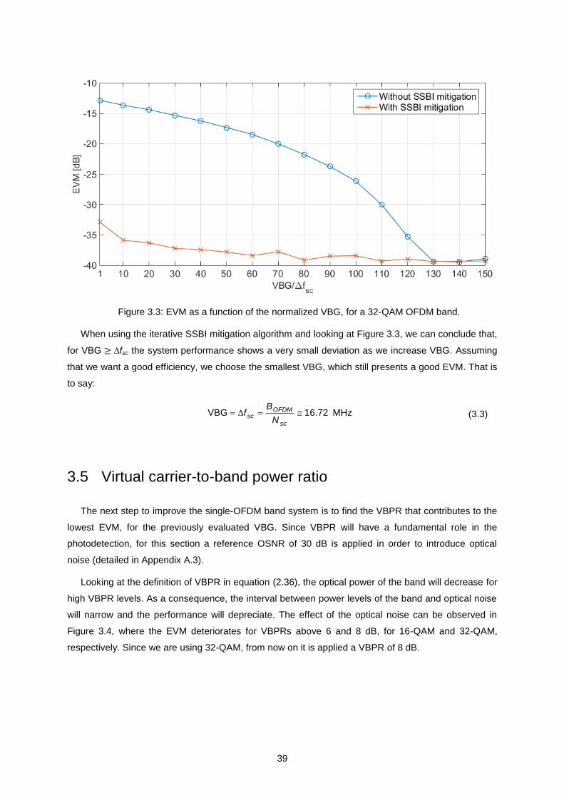
39
Figure 3.3: EVM as a function of the normalized VBG, for a 32-QAM OFDM band.
When using the iterative SSBI mitigation algorithm and looking at Figure 3.3, we can conclude that,
for VBG ≥ ∆fsc the system performance shows a very small deviation as we increase VBG. Assuming
that we want a good efficiency, we choose the smallest VBG, which still presents a good EVM. That is
to say:
VBG 16.72OFDMsc
sc
Bf
N MHz (3.3)
3.5 Virtual carrier-to-band power ratio
The next step to improve the single-OFDM band system is to find the VBPR that contributes to the
lowest EVM, for the previously evaluated VBG. Since VBPR will have a fundamental role in the
photodetection, for this section a reference OSNR of 30 dB is applied in order to introduce optical
noise (detailed in Appendix A.3).
Looking at the definition of VBPR in equation (2.36), the optical power of the band will decrease for
high VBPR levels. As a consequence, the interval between power levels of the band and optical noise
will narrow and the performance will depreciate. The effect of the optical noise can be observed in
Figure 3.4, where the EVM deteriorates for VBPRs above 6 and 8 dB, for 16-QAM and 32-QAM,
respectively. Since we are using 32-QAM, from now on it is applied a VBPR of 8 dB.
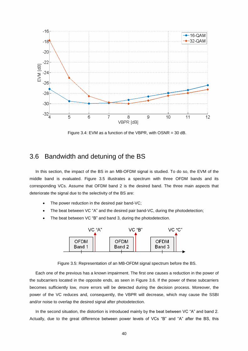
40
Figure 3.4: EVM as a function of the VBPR, with OSNR = 30 dB.
3.6 Bandwidth and detuning of the BS
In this section, the impact of the BS in an MB-OFDM signal is studied. To do so, the EVM of the
middle band is evaluated. Figure 3.5 illustrates a spectrum with three OFDM bands and its
corresponding VCs. Assume that OFDM band 2 is the desired band. The three main aspects that
deteriorate the signal due to the selectivity of the BS are:
The power reduction in the desired pair band-VC;
The beat between VC “A” and the desired pair band-VC, during the photodetection;
The beat between VC “B” and band 3, during the photodetection.
Figure 3.5: Representation of an MB-OFDM signal spectrum before the BS.
Each one of the previous has a known impairment. The first one causes a reduction in the power of
the subcarriers located in the opposite ends, as seen in Figure 3.6. If the power of these subcarriers
becomes sufficiently low, more errors will be detected during the decision process. Moreover, the
power of the VC reduces and, consequently, the VBPR will decrease, which may cause the SSBI
and/or noise to overlap the desired signal after photodetection.
In the second situation, the distortion is introduced mainly by the beat between VC “A” and band 2.
Actually, due to the great difference between power levels of VCs “B” and “A” after the BS, this
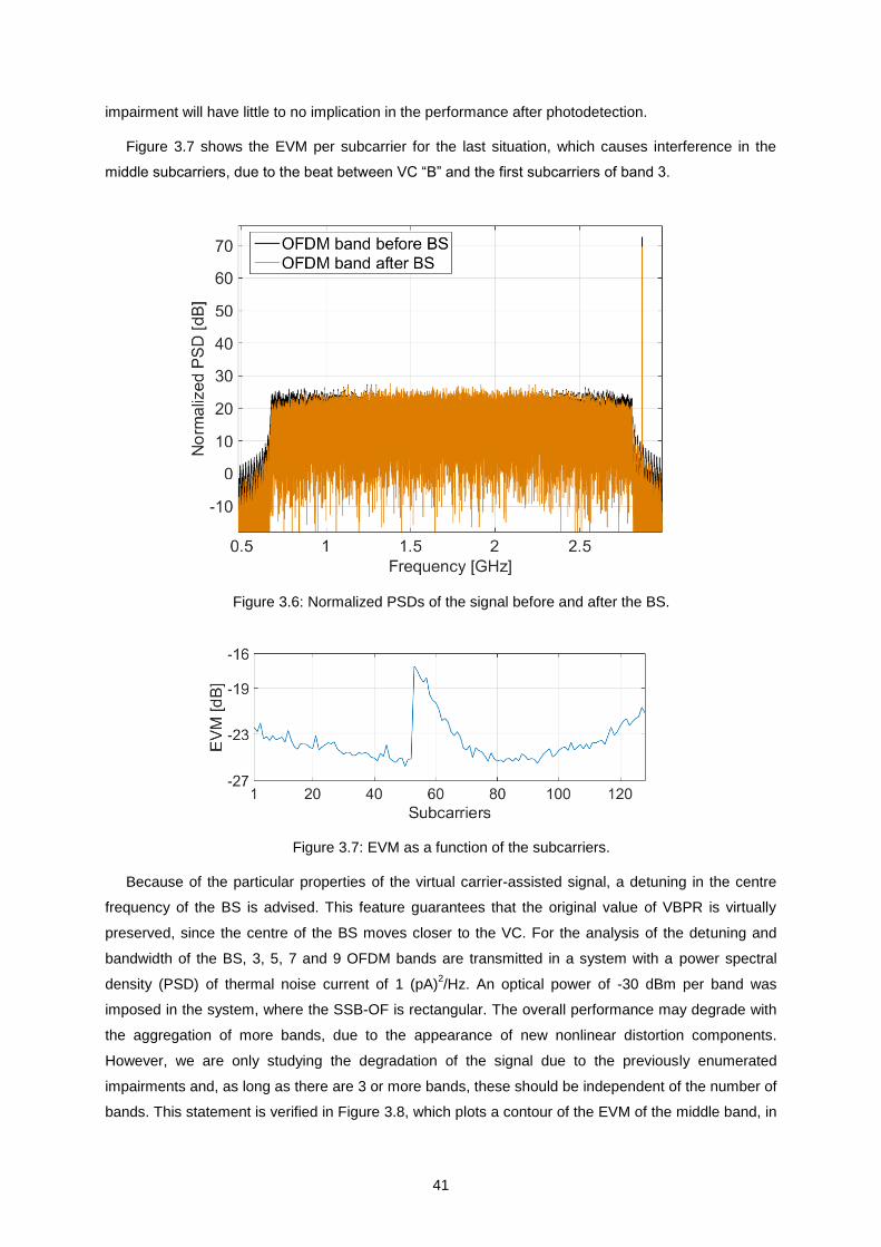
41
impairment will have little to no implication in the performance after photodetection.
Figure 3.7 shows the EVM per subcarrier for the last situation, which causes interference in the
middle subcarriers, due to the beat between VC “B” and the first subcarriers of band 3.
Figure 3.6: Normalized PSDs of the signal before and after the BS.
Figure 3.7: EVM as a function of the subcarriers.
Because of the particular properties of the virtual carrier-assisted signal, a detuning in the centre
frequency of the BS is advised. This feature guarantees that the original value of VBPR is virtually
preserved, since the centre of the BS moves closer to the VC. For the analysis of the detuning and
bandwidth of the BS, 3, 5, 7 and 9 OFDM bands are transmitted in a system with a power spectral
density (PSD) of thermal noise current of 1 (pA)2/Hz. An optical power of -30 dBm per band was
imposed in the system, where the SSB-OF is rectangular. The overall performance may degrade with
the aggregation of more bands, due to the appearance of new nonlinear distortion components.
However, we are only studying the degradation of the signal due to the previously enumerated
impairments and, as long as there are 3 or more bands, these should be independent of the number of
bands. This statement is verified in Figure 3.8, which plots a contour of the EVM of the middle band, in
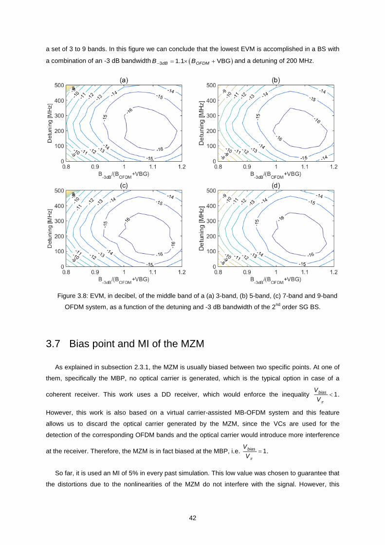
42
a set of 3 to 9 bands. In this figure we can conclude that the lowest EVM is accomplished in a BS with
a combination of an -3 dB bandwidth 3 1.1 VBGdB OFDMB B and a detuning of 200 MHz.
Figure 3.8: EVM, in decibel, of the middle band of a (a) 3-band, (b) 5-band, (c) 7-band and 9-band
OFDM system, as a function of the detuning and -3 dB bandwidth of the 2nd
order SG BS.
3.7 Bias point and MI of the MZM
As explained in subsection 2.3.1, the MZM is usually biased between two specific points. At one of
them, specifically the MBP, no optical carrier is generated, which is the typical option in case of a
coherent receiver. This work uses a DD receiver, which would enforce the inequality
1biasV
V.
However, this work is also based on a virtual carrier-assisted MB-OFDM system and this feature
allows us to discard the optical carrier generated by the MZM, since the VCs are used for the
detection of the corresponding OFDM bands and the optical carrier would introduce more interference
at the receiver. Therefore, the MZM is in fact biased at the MBP, i.e.
1biasV
V.
So far, it is used an MI of 5% in every past simulation. This low value was chosen to guarantee that
the distortions due to the nonlinearities of the MZM do not interfere with the signal. However, this

43
effect must be taken into account in order to optimize the performance of the MB-OFDM system and
the optimal MI must be estimated.
In [30], Cruz et al. modelled an ultra-dense DD SSB MB-OFDM system and evaluated the
maximum power allowed in a fibre, considering the four-wave mixing (FWM) as the main nonlinear
fibre effect. They demonstrated that the FWM limits the average power per slot (i.e. pair band-VC)
in -13.5 dBm, in a network with six spans of 40 km each, using a 32-OFDM bands system. We do not
emulate the penalty imposed by the FWM in the model, nevertheless we will use the results in [30] to
impose a maximum power into the fibre of -13.5 dBm.
Using the instance above, we impose the power for the farthest length of network in the next
simulations (i.e. -13.5 dBm per slot, in a six spans network of 240 km) and use the EVM to estimate an
ideal MI. The EVM was calculated directly at the output of the last OA in Figure 2.17, as a result no
access network was considered. Moreover, each OA compensates the fibre attenuation and the
insertion losses of each RU, so the metro network is balanced. More details on the numerical
parameters of the model of the network are found in Table 3.4.
Table 3.4: Parameters of some elements inside the metro-access network.
Insertion losses of the RU [dB] 5.5
Fibre attenuation [dB/km] 0.25
Gain of each OA [dB] 5.5 + 0.25×40 = 15.5
Noise figure of the OA [dB] 4
By the MI definition in equation (2.25), we expect that very small MI values would result in poor
performances, because the noise would overlap the signal. Similarly, as the MI increases, the system
performance would degrade, due to the field transfer characteristic of the IM, because for high
voltages the MZM works outside the zone of virtually linear modulation.
Figure 3.9 pictures the evolution of the EVM as a function of the MI. For 1 OFDM band and MIs
greater than 6%, the EVM is almost constant. However, when emitting more bands in the same MZM,
its nonlinear effects start to inflict distortions in the signal. We choose 8% for the MI in this work, since
it is the value which results in the best EVM, considering the worst case, i.e. 4 bands per MZM.
As stated above, the simulations of Figure 3.9 considered the top limit of average power and the
farthest length of spans. It can be seen that the EVM does not meet the value to which the BER is
3.8×10⁻³
, i.e. EVM = -18.2 dB. Therefore, the next goal is to decrease the length of the spans, until an
acceptable performance is achieved.
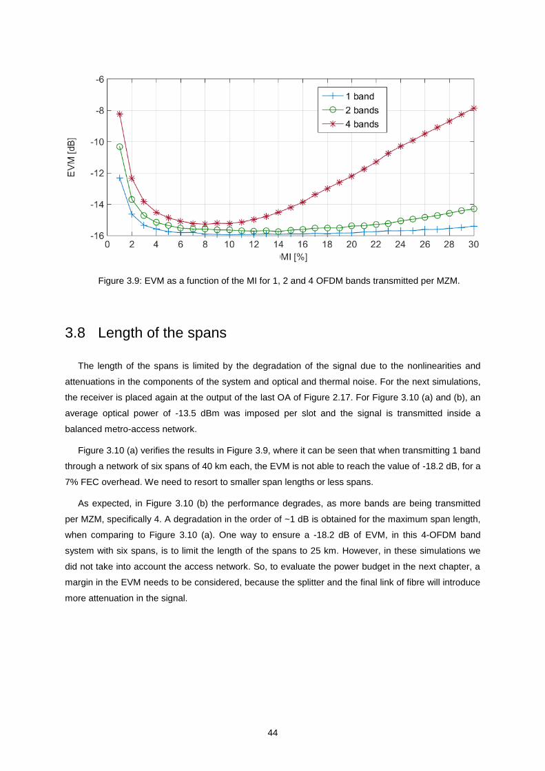
44
Figure 3.9: EVM as a function of the MI for 1, 2 and 4 OFDM bands transmitted per MZM.
3.8 Length of the spans
The length of the spans is limited by the degradation of the signal due to the nonlinearities and
attenuations in the components of the system and optical and thermal noise. For the next simulations,
the receiver is placed again at the output of the last OA of Figure 2.17. For Figure 3.10 (a) and (b), an
average optical power of -13.5 dBm was imposed per slot and the signal is transmitted inside a
balanced metro-access network.
Figure 3.10 (a) verifies the results in Figure 3.9, where it can be seen that when transmitting 1 band
through a network of six spans of 40 km each, the EVM is not able to reach the value of -18.2 dB, for a
7% FEC overhead. We need to resort to smaller span lengths or less spans.
As expected, in Figure 3.10 (b) the performance degrades, as more bands are being transmitted
per MZM, specifically 4. A degradation in the order of ~1 dB is obtained for the maximum span length,
when comparing to Figure 3.10 (a). One way to ensure a -18.2 dB of EVM, in this 4-OFDM band
system with six spans, is to limit the length of the spans to 25 km. However, in these simulations we
did not take into account the access network. So, to evaluate the power budget in the next chapter, a
margin in the EVM needs to be considered, because the splitter and the final link of fibre will introduce
more attenuation in the signal.
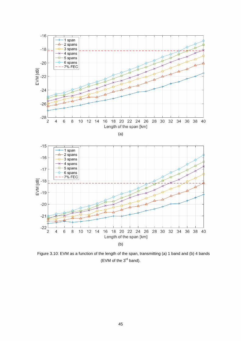
45
(a)
(b)
Figure 3.10: EVM as a function of the length of the span, transmitting (a) 1 band and (b) 4 bands
(EVM of the 3rd
band).

46
3.9 Conclusion
In this chapter, we selected the numerical parameters of the system, through simulation in
MATLAB®. The modulation scheme was sorted out based on the selectivity of the 2
nd order SG OF,
used as BS. Also, the best VBG and VBPR were assessed using the EVM as a figure of merit.
The impact of varying the bandwidth and detuning of the BS was shown. The detuning was
described as an important feature to counteract the remaining power of the VC from the previous
band.
It was concluded that the MZM for this specific metro-access network has the best performance
when it is biased at the MBP and has an MI equal to 8%. A maximum of 4 OFDM bands per MZM was
also imposed.
Finally, the length of the network was estimated. In Table 3.5 we present the maximum length of
each span to ensure the acceptable BER of 3.8×10⁻³
, from the analysis of Figure 3.10. It was
concluded that choosing smaller spans or less spans is essential because, until now, we are not
considering the attenuations present in the distribution link.
From the results of this chapter, we have built Table 3.6, where the optimal parameters for this
virtual carrier-assisted MB-OFDM metro-access network are presented.
Table 3.5: Maximum length of spans to ensure a BER of 3.8×10⁻³
.
Number of spans Maximum length of span [km]
(for 1 band)
Maximum length of span [km]
(for 4 bands)
1 40 40
2 40 40
3 40 35
4 40 31
5 36 28
6 34 26
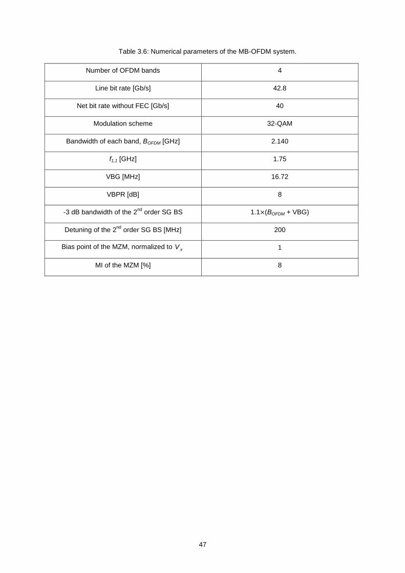
47
Table 3.6: Numerical parameters of the MB-OFDM system.
Number of OFDM bands 4
Line bit rate [Gb/s] 42.8
Net bit rate without FEC [Gb/s] 40
Modulation scheme 32-QAM
Bandwidth of each band, BOFDM [GHz] 2.140
f1,1 [GHz] 1.75
VBG [MHz] 16.72
VBPR [dB] 8
-3 dB bandwidth of the 2nd
order SG BS 1.1×(BOFDM + VBG)
Detuning of the 2nd
order SG BS [MHz] 200
Bias point of the MZM, normalized to V 1
MI of the MZM [%] 8


49
Chapter 4
SSB-OF optimization and power
budget assessment SSB-OF optimization and power budget assessment 4
In this chapter, the SSB-OF is optimized resorting to the EVM of the received symbols and the
power budget of the metro-access network is assessed. The latter is evaluated using the exhaustive
Gaussian approach (EGA) (detailed in Appendix B.2).
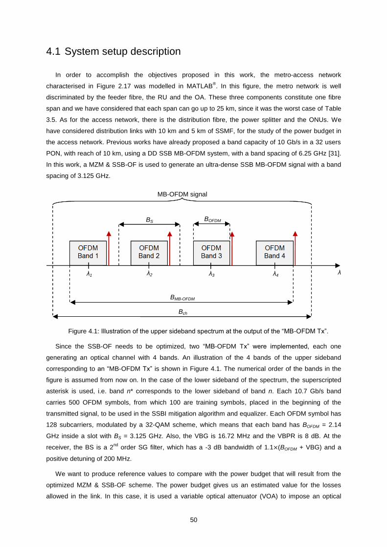
50
4.1 System setup description
In order to accomplish the objectives proposed in this work, the metro-access network
characterised in Figure 2.17 was modelled in MATLAB®. In this figure, the metro network is well
discriminated by the feeder fibre, the RU and the OA. These three components constitute one fibre
span and we have considered that each span can go up to 25 km, since it was the worst case of Table
3.5. As for the access network, there is the distribution fibre, the power splitter and the ONUs. We
have considered distribution links with 10 km and 5 km of SSMF, for the study of the power budget in
the access network. Previous works have already proposed a band capacity of 10 Gb/s in a 32 users
PON, with reach of 10 km, using a DD SSB MB-OFDM system, with a band spacing of 6.25 GHz [31].
In this work, a MZM & SSB-OF is used to generate an ultra-dense SSB MB-OFDM signal with a band
spacing of 3.125 GHz.
Figure 4.1: Illustration of the upper sideband spectrum at the output of the “MB-OFDM Tx”.
Since the SSB-OF needs to be optimized, two “MB-OFDM Tx” were implemented, each one
generating an optical channel with 4 bands. An illustration of the 4 bands of the upper sideband
corresponding to an “MB-OFDM Tx” is shown in Figure 4.1. The numerical order of the bands in the
figure is assumed from now on. In the case of the lower sideband of the spectrum, the superscripted
asterisk is used, i.e. band n* corresponds to the lower sideband of band n. Each 10.7 Gb/s band
carries 500 OFDM symbols, from which 100 are training symbols, placed in the beginning of the
transmitted signal, to be used in the SSBI mitigation algorithm and equalizer. Each OFDM symbol has
128 subcarriers, modulated by a 32-QAM scheme, which means that each band has BOFDM = 2.14
GHz inside a slot with BS = 3.125 GHz. Also, the VBG is 16.72 MHz and the VBPR is 8 dB. At the
receiver, the BS is a 2nd
order SG filter, which has a -3 dB bandwidth of 1.1×(BOFDM + VBG) and a
positive detuning of 200 MHz.
We want to produce reference values to compare with the power budget that will result from the
optimized MZM & SSB-OF scheme. The power budget gives us an estimated value for the losses
allowed in the link. In this case, it is used a variable optical attenuator (VOA) to impose an optical
MB-OFDM signal
BS BOFDM
BMB-OFDM
Bch
λ1 λ2 λ3 λ4 λ
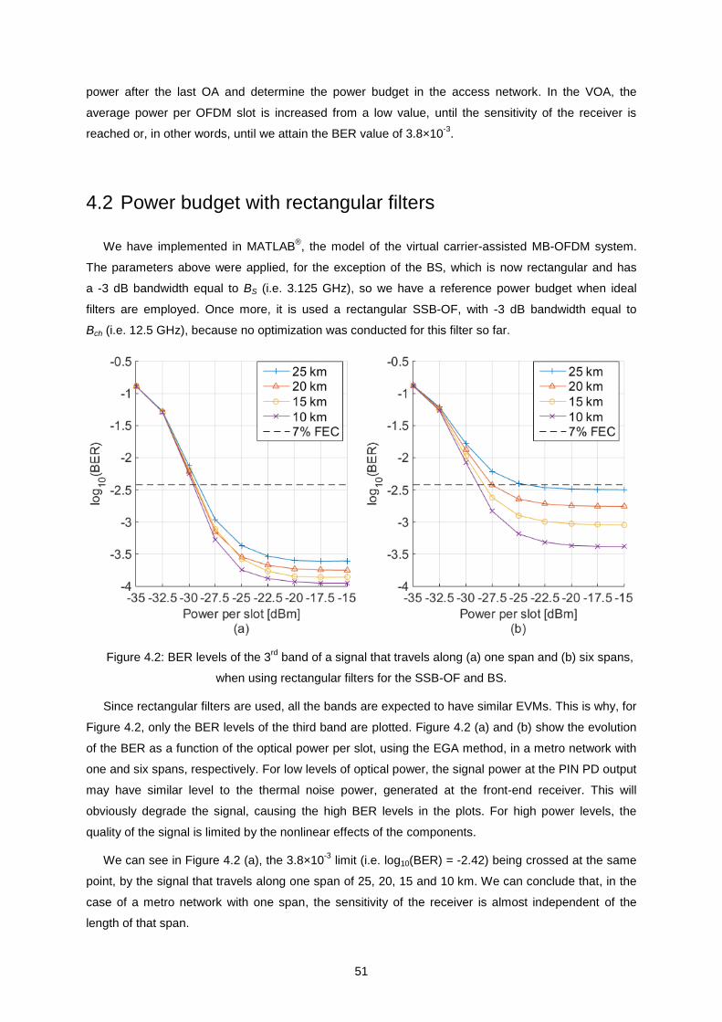
51
power after the last OA and determine the power budget in the access network. In the VOA, the
average power per OFDM slot is increased from a low value, until the sensitivity of the receiver is
reached or, in other words, until we attain the BER value of 3.8×10⁻³
.
4.2 Power budget with rectangular filters
We have implemented in MATLAB®, the model of the virtual carrier-assisted MB-OFDM system.
The parameters above were applied, for the exception of the BS, which is now rectangular and has
a -3 dB bandwidth equal to BS (i.e. 3.125 GHz), so we have a reference power budget when ideal
filters are employed. Once more, it is used a rectangular SSB-OF, with -3 dB bandwidth equal to
Bch (i.e. 12.5 GHz), because no optimization was conducted for this filter so far.
Figure 4.2: BER levels of the 3rd
band of a signal that travels along (a) one span and (b) six spans,
when using rectangular filters for the SSB-OF and BS.
Since rectangular filters are used, all the bands are expected to have similar EVMs. This is why, for
Figure 4.2, only the BER levels of the third band are plotted. Figure 4.2 (a) and (b) show the evolution
of the BER as a function of the optical power per slot, using the EGA method, in a metro network with
one and six spans, respectively. For low levels of optical power, the signal power at the PIN PD output
may have similar level to the thermal noise power, generated at the front-end receiver. This will
obviously degrade the signal, causing the high BER levels in the plots. For high power levels, the
quality of the signal is limited by the nonlinear effects of the components.
We can see in Figure 4.2 (a), the 3.8×10⁻³
limit (i.e. log10(BER) = -2.42) being crossed at the same
point, by the signal that travels along one span of 25, 20, 15 and 10 km. We can conclude that, in the
case of a metro network with one span, the sensitivity of the receiver is almost independent of the
length of that span.
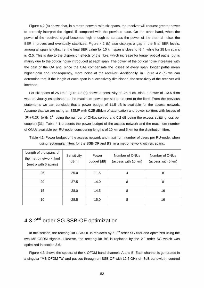
52
Figure 4.2 (b) shows that, in a metro network with six spans, the receiver will request greater power
to correctly interpret the signal, if compared with the previous case. On the other hand, when the
power of the received signal becomes high enough to surpass the power of the thermal noise, the
BER improves and eventually stabilizes. Figure 4.2 (b) also displays a gap in the final BER levels,
among all span lengths, i.e. the final BER value for 10 km span is close to -3.4, while for 25 km spans
is -2.5. This is due to the dispersion effects of the fibre, which increase for longer optical paths, but is
mainly due to the optical noise introduced at each span. The power of the optical noise increases with
the gain of the OA and, since the OAs compensate the losses of every span, longer paths mean
higher gain and, consequently, more noise at the receiver. Additionally, in Figure 4.2 (b) we can
determine that, if the length of each span is successively diminished, the sensitivity of the receiver will
increase.
For six spans of 25 km, Figure 4.2 (b) shows a sensitivity of -25 dBm. Also, a power of -13.5 dBm
was previously established as the maximum power per slot to be sent to the fibre. From the previous
statements we can conclude that a power budget of 11.5 dB is available for the access network.
Assume that we are using an SSMF with 0.25 dB/km of attenuation and power splitters with losses of
3 0.2k k (with 2 k being the number of ONUs served and 0.2 dB being the excess splitting loss per
coupler) [31]. Table 4.1 presents the power budget of the access network and the maximum number
of ONUs available per RU-node, considering lengths of 10 km and 5 km for the distribution fibre.
Table 4.1: Power budget of the access network and maximum number of users per RU-node, when
using rectangular filters for the SSB-OF and BS, in a metro network with six spans.
Length of the spans of
the metro network [km]
(metro with 6 spans)
Sensitivity
[dBm]
Power
budget [dB]
Number of ONUs
(access with 10 km)
Number of ONUs
(access with 5 km)
25 -25.0 11.5 4 8
20 -27.5 14.0 8 8
15 -28.0 14.5 8 16
10 -28.5 15.0 8 16
4.3 2nd
order SG SSB-OF optimization
In this section, the rectangular SSB-OF is replaced by a 2nd
order SG filter and optimized using the
two MB-OFDM signals. Likewise, the rectangular BS is replaced by the 2nd
order SG which was
optimized in section 3.6.
Figure 4.3 shows the spectra of the 4-OFDM band channels A and B. Each channel is generated in
a singular “MB-OFDM Tx” and passes through an SSB-OF with 12.5 GHz of -3dB bandwidth, centred
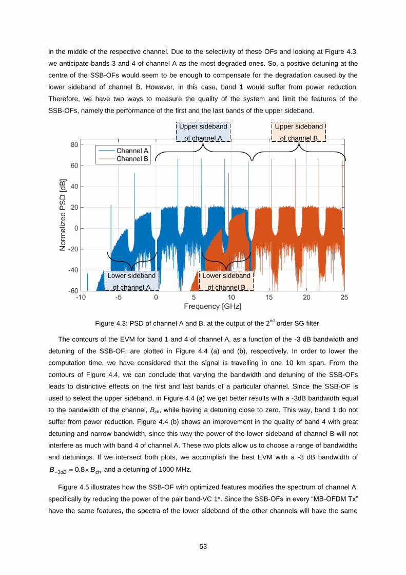
53
in the middle of the respective channel. Due to the selectivity of these OFs and looking at Figure 4.3,
we anticipate bands 3 and 4 of channel A as the most degraded ones. So, a positive detuning at the
centre of the SSB-OFs would seem to be enough to compensate for the degradation caused by the
lower sideband of channel B. However, in this case, band 1 would suffer from power reduction.
Therefore, we have two ways to measure the quality of the system and limit the features of the
SSB-OFs, namely the performance of the first and the last bands of the upper sideband.
Figure 4.3: PSD of channel A and B, at the output of the 2nd
order SG filter.
The contours of the EVM for band 1 and 4 of channel A, as a function of the -3 dB bandwidth and
detuning of the SSB-OF, are plotted in Figure 4.4 (a) and (b), respectively. In order to lower the
computation time, we have considered that the signal is travelling in one 10 km span. From the
contours of Figure 4.4, we can conclude that varying the bandwidth and detuning of the SSB-OFs
leads to distinctive effects on the first and last bands of a particular channel. Since the SSB-OF is
used to select the upper sideband, in Figure 4.4 (a) we get better results with a -3dB bandwidth equal
to the bandwidth of the channel, Bch, while having a detuning close to zero. This way, band 1 do not
suffer from power reduction. Figure 4.4 (b) shows an improvement in the quality of band 4 with great
detuning and narrow bandwidth, since this way the power of the lower sideband of channel B will not
interfere as much with band 4 of channel A. These two plots allow us to choose a range of bandwidths
and detunings. If we intersect both plots, we accomplish the best EVM with a -3 dB bandwidth of
3 0.8dB chB B and a detuning of 1000 MHz.
Figure 4.5 illustrates how the SSB-OF with optimized features modifies the spectrum of channel A,
specifically by reducing the power of the pair band-VC 1*. Since the SSB-OFs in every “MB-OFDM Tx”
have the same features, the spectra of the lower sideband of the other channels will have the same
Upper sideband
of channel B
Lower sideband
of channel B
Lower sideband
of channel A
Upper sideband
of channel A
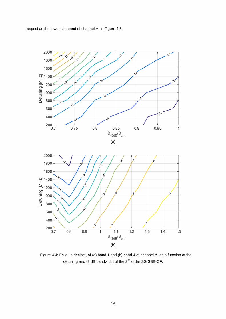
54
aspect as the lower sideband of channel A, in Figure 4.5.
(a)
(b)
Figure 4.4: EVM, in decibel, of (a) band 1 and (b) band 4 of channel A, as a function of the
detuning and -3 dB bandwidth of the 2nd
order SG SSB-OF.
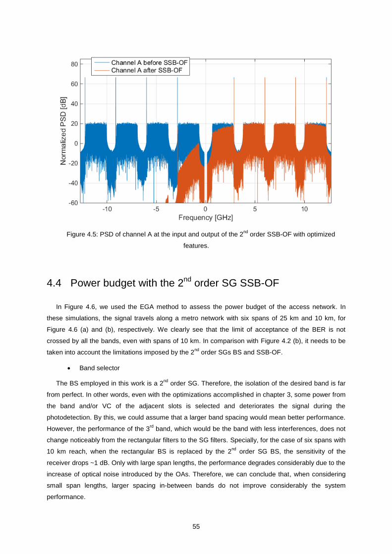
55
Figure 4.5: PSD of channel A at the input and output of the 2nd
order SSB-OF with optimized
features.
4.4 Power budget with the 2nd
order SG SSB-OF
In Figure 4.6, we used the EGA method to assess the power budget of the access network. In
these simulations, the signal travels along a metro network with six spans of 25 km and 10 km, for
Figure 4.6 (a) and (b), respectively. We clearly see that the limit of acceptance of the BER is not
crossed by all the bands, even with spans of 10 km. In comparison with Figure 4.2 (b), it needs to be
taken into account the limitations imposed by the 2nd
order SGs BS and SSB-OF.
Band selector
The BS employed in this work is a 2nd
order SG. Therefore, the isolation of the desired band is far
from perfect. In other words, even with the optimizations accomplished in chapter 3, some power from
the band and/or VC of the adjacent slots is selected and deteriorates the signal during the
photodetection. By this, we could assume that a larger band spacing would mean better performance.
However, the performance of the 3rd
band, which would be the band with less interferences, does not
change noticeably from the rectangular filters to the SG filters. Specially, for the case of six spans with
10 km reach, when the rectangular BS is replaced by the 2nd
order SG BS, the sensitivity of the
receiver drops ~1 dB. Only with large span lengths, the performance degrades considerably due to the
increase of optical noise introduced by the OAs. Therefore, we can conclude that, when considering
small span lengths, larger spacing in-between bands do not improve considerably the system
performance.
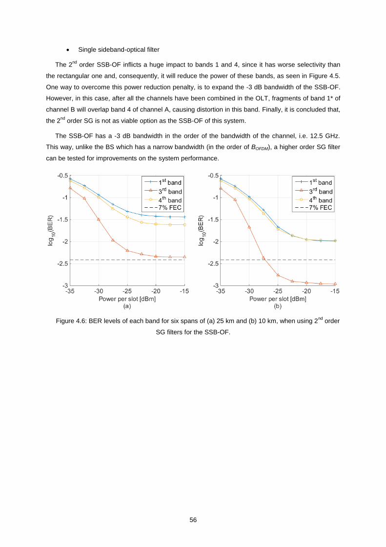
56
Single sideband-optical filter
The 2nd
order SSB-OF inflicts a huge impact to bands 1 and 4, since it has worse selectivity than
the rectangular one and, consequently, it will reduce the power of these bands, as seen in Figure 4.5.
One way to overcome this power reduction penalty, is to expand the -3 dB bandwidth of the SSB-OF.
However, in this case, after all the channels have been combined in the OLT, fragments of band 1* of
channel B will overlap band 4 of channel A, causing distortion in this band. Finally, it is concluded that,
the 2nd
order SG is not as viable option as the SSB-OF of this system.
The SSB-OF has a -3 dB bandwidth in the order of the bandwidth of the channel, i.e. 12.5 GHz.
This way, unlike the BS which has a narrow bandwidth (in the order of BOFDM), a higher order SG filter
can be tested for improvements on the system performance.
Figure 4.6: BER levels of each band for six spans of (a) 25 km and (b) 10 km, when using 2nd
order
SG filters for the SSB-OF.
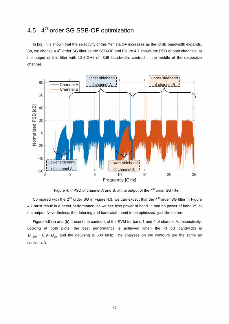
57
4.5 4th order SG SSB-OF optimization
In [32], it is shown that the selectivity of this Yenista OF increases as the -3 dB bandwidth expands.
So, we choose a 4th order SG filter as the SSB-OF and Figure 4.7 shows the PSD of both channels, at
the output of this filter with 12.5 GHz of -3dB bandwidth, centred in the middle of the respective
channel.
Figure 4.7: PSD of channel A and B, at the output of the 4th order SG filter.
Compared with the 2nd
order SG in Figure 4.3, we can expect that the 4th order SG filter in Figure
4.7 must result in a better performance, as we see less power of band 1* and no power of band 2*, at
the output. Nevertheless, the detuning and bandwidth need to be optimized, just like before.
Figure 4.8 (a) and (b) present the contours of the EVM for band 1 and 4 of channel A, respectively.
Looking at both plots, the best performance is achieved when the -3 dB bandwidth is
3 0.9dB chB B and the detuning is 600 MHz. The analyses on the contours are the same as
section 4.3.
Upper sideband
of channel B
Lower sideband
of channel B
Lower sideband
of channel A
Upper sideband
of channel A
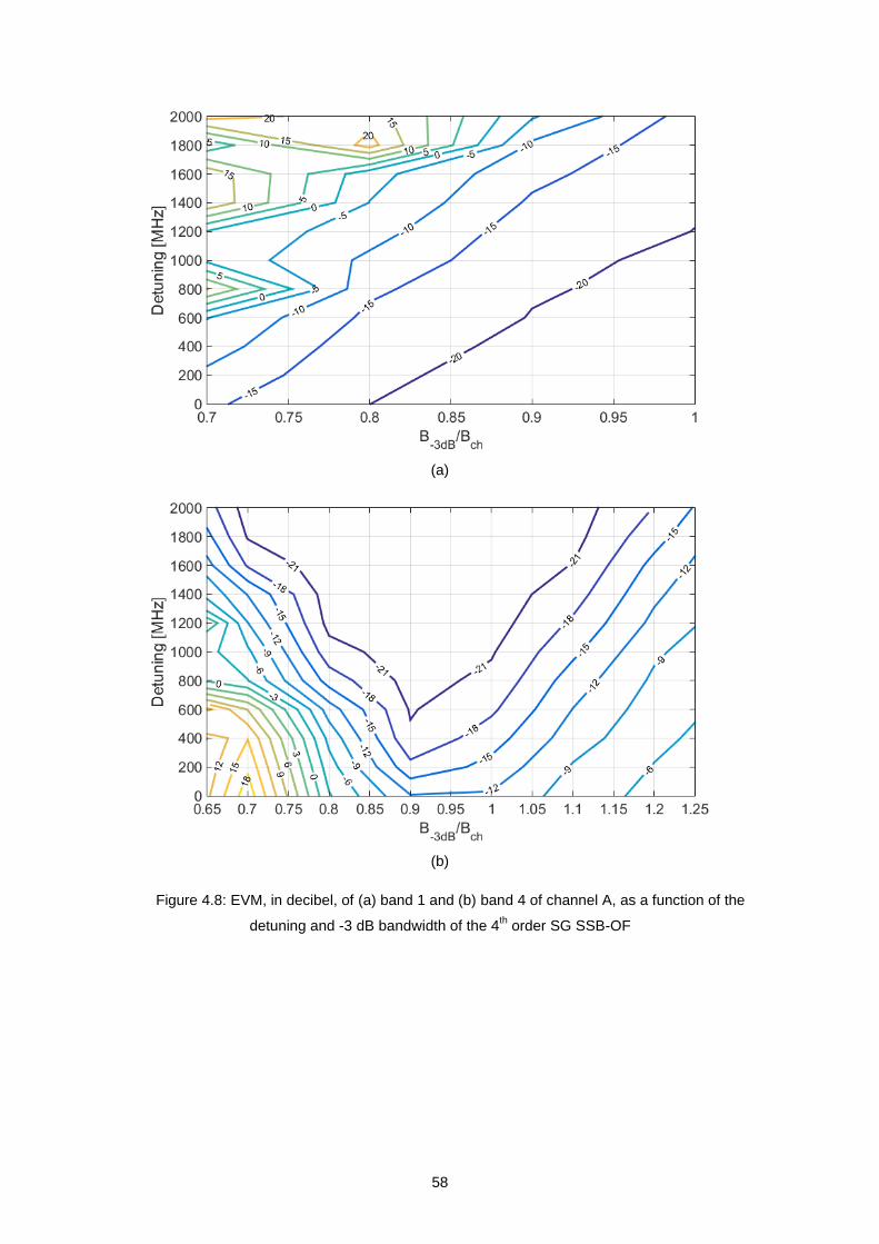
58
(a)
(b)
Figure 4.8: EVM, in decibel, of (a) band 1 and (b) band 4 of channel A, as a function of the
detuning and -3 dB bandwidth of the 4th order SG SSB-OF
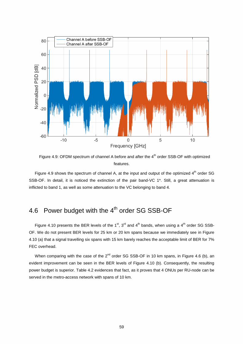
59
Figure 4.9: OFDM spectrum of channel A before and after the 4th order SSB-OF with optimized
features.
Figure 4.9 shows the spectrum of channel A, at the input and output of the optimized 4th order SG
SSB-OF. In detail, it is noticed the extinction of the pair band-VC 1*. Still, a great attenuation is
inflicted to band 1, as well as some attenuation to the VC belonging to band 4.
4.6 Power budget with the 4th order SG SSB-OF
Figure 4.10 presents the BER levels of the 1st, 3
rd and 4
th bands, when using a 4
th order SG SSB-
OF. We do not present BER levels for 25 km or 20 km spans because we immediately see in Figure
4.10 (a) that a signal travelling six spans with 15 km barely reaches the acceptable limit of BER for 7%
FEC overhead.
When comparing with the case of the 2nd
order SG SSB-OF in 10 km spans, in Figure 4.6 (b), an
evident improvement can be seen in the BER levels of Figure 4.10 (b). Consequently, the resulting
power budget is superior. Table 4.2 evidences that fact, as it proves that 4 ONUs per RU-node can be
served in the metro-access network with spans of 10 km.
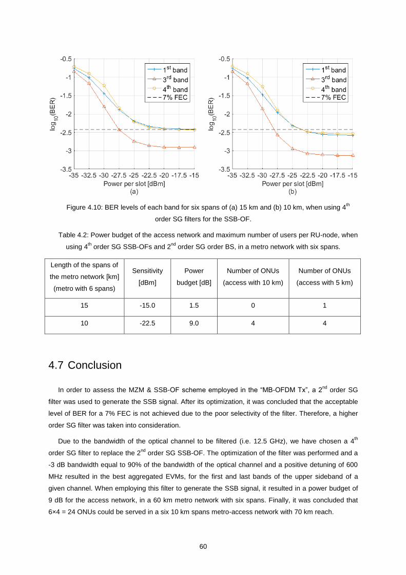
60
Figure 4.10: BER levels of each band for six spans of (a) 15 km and (b) 10 km, when using 4th
order SG filters for the SSB-OF.
Table 4.2: Power budget of the access network and maximum number of users per RU-node, when
using 4th order SG SSB-OFs and 2
nd order SG order BS, in a metro network with six spans.
Length of the spans of
the metro network [km]
(metro with 6 spans)
Sensitivity
[dBm]
Power
budget [dB]
Number of ONUs
(access with 10 km)
Number of ONUs
(access with 5 km)
15 -15.0 1.5 0 1
10 -22.5 9.0 4 4
4.7 Conclusion
In order to assess the MZM & SSB-OF scheme employed in the “MB-OFDM Tx”, a 2nd
order SG
filter was used to generate the SSB signal. After its optimization, it was concluded that the acceptable
level of BER for a 7% FEC is not achieved due to the poor selectivity of the filter. Therefore, a higher
order SG filter was taken into consideration.
Due to the bandwidth of the optical channel to be filtered (i.e. 12.5 GHz), we have chosen a 4th
order SG filter to replace the 2nd
order SG SSB-OF. The optimization of the filter was performed and a
-3 dB bandwidth equal to 90% of the bandwidth of the optical channel and a positive detuning of 600
MHz resulted in the best aggregated EVMs, for the first and last bands of the upper sideband of a
given channel. When employing this filter to generate the SSB signal, it resulted in a power budget of
9 dB for the access network, in a 60 km metro network with six spans. Finally, it was concluded that
6×4 = 24 ONUs could be served in a six 10 km spans metro-access network with 70 km reach.

61
Obviously, the amount of users served in this system is insufficient for the next generation PONs,
especially when solutions of 32 users or more are available [31]. We already saw that larger band
spacing would not improve the system performance. However, as the degradation present in the 1st
and 4th bands is mostly induced by the SSB-OF, we can conclude that a larger spacing in-between
channels would improve the system performance. In other words, a larger channel spacing would
relax the constraints on the selectivity of the SSB-OF and, consequently, only negligible portions of the
adjacent channel would overlap the desired channel.


63
Chapter 5
Conclusion
Conclusion 5
In this chapter, the final conclusions are presented, as well as the suggestions for future work.
64
5.1 Final conclusions
In this work, the performance of the single-arm chirpless MZM followed by an SSB-OF, in an
ultra-dense DD SSB MB-OFDM metro-access network capable of guaranteeing 10 Gb/s per user, was
evaluated.
In chapter 2, we have reported the fundamentals of the MB-OFDM signal. The OFDM transmitter,
the OFDM DD receiver and the equipment required to generate the SSB signal was detailed. In the
latter, the MZM & OF scheme was presented. To have a cost-effective network, it was implemented a
DD receiver at the system and it were used virtual-carriers, in every OFDM band, to assist the
photodetection of the optical signal. An iterative DSP used to mitigate the SSBI was suggested,
implemented in the model and the improvement in the system performance was evaluated. Finally, it
was shown the architecture of the MB-OFDM metro-access network, followed by a brief description of
its elements, namely the CO, RU and ONU. This model was implemented in MATLAB® and used for
the following simulations.
In chapter 3, we optimized the parameters of the virtual-carrier assisted MB-OFDM system.
Considering a band capacity of 10 Gb/s, with a 7% FEC overhead, a band spacing of 3.125 GHz and
a 2nd
order SG BS, we have chosen a 32-QAM scheme, which resulted in a bandwidth of 2.14 GHz.
The impact of the VBPR and VBG on the performance of a 4-OFDM band system was analysed and it
was concluded that the best VBPR is 8 dB, whereas a VBG equal to the spacing between subcarriers
(i.e. 16.72 MHz) is chosen to maximise the spectral efficiency. With 1.75 GHz as the frequency of the
first band, the optimization of the parameters of the BS resulted in a -3 dB bandwidth 10% larger than
the bandwidth of the OFDM band plus the VC, and in a positive detuning equal to 200 MHz. Since we
used virtual-carriers to assist the photodetection, the MZM was biased at the MBP. A power per slot
(i.e. pair band-VC) of -13.5 dBm was imposed in a signal, traveling six spans of 40 km each, and the
impact of the MI, on the performance of the 3rd
band of the 4-OFDM band system, defined its optimum
value. An optimized MI of 8% was attained. In addition, it was concluded that, to guarantee a BER of
3.8×10⁻³
(i.e. EVM = -18.2 dB) in the metro network with six spans, the length of each span needed to
be below 27 km.
In chapter 4, we assessed the power budget of the access network using rectangular filters for the
BS and SSB-OF. In a six spans metro network of 60 km reach, it was obtained a power budget of
15 dB, which guarantees 10 Gb/s per user to 8 and 16 ONUs, for an access network of 10 km and
5 km, respectively. Later, the rectangular filters were replaced by the previously optimized BS and the
optimization of a 2nd
order SG SSB-OF was accomplished. However, the analysis on the sensitivity of
the receiver determined that no ONU could be served. A higher order SG filter was chosen, namely a
4th order SG SSB-OF, and its optimization resulted in a -3 dB bandwidth of 11.25 GHz and in a
positive detuning of 600 MHz. A power budget of 9 dB was obtained, which resulted in a guaranteed
service of 10 Gb/s per user to 4 ONUs per RU-node. Thus, it was concluded that the proposed system
is able to guarantee a band capacity of 10 Gb/s per user to 24 ONUs, in a metro network with six
spans of 10 km and an access network with 10 km reach.

65
5.2 Future Works
Subsequently to the work performed along this dissertation, the following topics are suggested as
future work:
To assess the power budget for fewer number of spans and different span lengths;
To implement a larger channel spacing in the MB-OFDM signal, allowing less constrains in
the SSB-OF features, and assess the performance of the system;
To implement, in this metro-access network, other structures capable of generating an
optical SSB signal and compare their performances with the results presented in this
dissertation;
To implement the nonlinear propagation effects in the transfer function of the fibre and
study the performance degradation;
To experimentally demonstrate the metro-access MB-OFDM integrated network, employing
the MZM & OF scheme.

67
References
References
[1] D. R. Anderson, L. M. Johnson and F. G. Bell, “Fundamentals of fiber optics,” in Troubleshooting
Optical-Fiber Networks: Understanding and Using Your Optical Time-Domain Reflectometer, 2nd
ed., USA, Elsevier, 2004.
[2] R. Ramaswami, K. Sivarajan and G. Sasaki, Optical Networks: A Practical Perspective, 3rd
ed.,
USA, Elsevier, 2010.
[3] I. Tomkos, “Metropolitan area optical networks,” IEEE Circuits & Devices Magazine, vol. 19, no. 4,
pp. 24-30, 2013.
[4] N. Cvijetic, “OFDM for next-generation optical access networks,” IEEE/OSA Journal of Lightwave
Technology, vol. 30, no. 4, pp. 384-398, 2012.
[5] A. Lovri , S. Aleksic, J. Lazaro, G. Beleffi and J. Prat, V. Polo, “Power efficiency of SARDANA and
other long-reach optical access networks,” 15th International Conference on Optical Network
Design and Modeling, Bologna, 2011.
[6] N. Ghazisaidi, M. Scheutzow and M. Maier, “Survivability analysis of next-generation passive
optical networks and fiber-wireless access networks,” IEEE Transactions on Reliability, vol. 60, no.
2, pp. 479-492, 2011.
[7] J. Prat, R. Soila, S. Spirou, P. Chanclou, A. Teixeira, G. Beleffi and I. Tomkos, The SARDANA
FTTH network, SARDANA Consortium, 2010.
[8] J. Lazaro, J. Prat, P. Chanclou, G. Beleffi, A. Teixeira, I. Tomkos and V. Koratzinos, “Scalable
extended reach PON,” Conference on Optical Fiber communication/National Fiber Optic Engineers
Conference, San Diego, 2008, paper OThL2.
[9] N. Cvijetic , M. Huang, E. Ip, Y. Huang, D. Qian and T. Wang, “1.2 Tb/s symmetric WDM-OFDMA-
PON over 90km straight SSMF and 1∶32 passive split with digitally-selective ONUs and coherent
receiver OLT,” Optical Fiber Communication Conference and Exposition and the National Fiber
Optic Engineers Conference, Los Angeles, 2011, paper PDPD7. [10] W. Shieh and I. Djordjevic, OFDM for Optical Communications, Elsevier, USA, 2010.
[11] K. Jong, H. Tsao and S. Lee, “Performance of OFDM signal for radio-over-fiber link adopting
electroabsorption modulator,” 14th OptoElectronics and Communications Conference, pp. 1-2,
Hong Kong, 2009, paper ThJ5.
[12] M. Sieben, J. Conradi and D. Dodds, “Optical single sideband transmission at 10Gb/s using only
electrical dispersion compensation,” IEEE/OSA Journal of Lightwave Technology, vol. 17, no. 10,
pp. 1742-1749, 1999.
68
[13] T. Alves and A. Cartaxo, “Transmission of OFDM-UWB radio signals in IM-DD optical fiber
communication systems employing optimized dual parallel Mach-Zehnder modulators,” Journal of
Optical Communications and Networking, vol. 5, no. 2, pp. 159-171, 2013.
[14] R. Chang, “Orthogonal frequency multiplexing data transmission system,” U.S. Patent 3 488 445,
1966.
[15] S. Weinstein and J. Salz, “Fourier transform communication systems,” Proceedings of the first
ACM Symposium on Problems in the Optimization of Data Communications Systems, Pine
Mountain, 1969.
[16] L. Cimini, “Analysis and simulation of a digital mobile channel using orthogonal frequency division
multiplexing,” IEEE Transactions on Communications, vol. 33, no. 7, pp. 665-675, 1985.
[17] B. Dixon, R. Pollard and S. Iezekeil, “Orthogonal frequency-division multiplexing in wireless
communication systems with multimode fiber feeds,” IEEE Transactions on Microwave Theory and
Techniques, vol. 49, pp. 1407-1409, 2001.
[18] W. Shieh, Q. Yang, Y. Ma, “107 Gb/s coherent optical OFDM transmission over 1000-km SSMF
fiber using orthogonal band multiplexing,” OSA Optics Express, vol. 16, n. 9, pp. 6378-6386, 2008.
[19] S. Blouza, E. Le Rouzic, N. Brochier and B. Cousin, “Optical multi-band OFDM switching
technology,” 17th European Conference on Networks and Optical Communications, Vilanova i la
Geltru, 2012, doi: 10.1109/NOC.2012.6249935.
[20] T. Alves, L. Mendes and A. Cartaxo, “High granularity multiband OFDM virtual carrier-assisted
direct-detection metro networks,” IEEE/OSA Journal of Lightwave Technology, vol. 33, no. 1, pp.
42-54, 2015.
[21] J. Armstrong, “OFDM for optical communications," IEEE/OSA Journal of Lightwave Technology,
vol. 27, pp. 189-204, 2009.
[22] E. L. Wooten, K. Kissa, A. Yi-Yan, E. Murphy, D. Lafaw, P. Hallemeier, D. Maack, D. Attanasio, D.
Fritz, G. McBrien and D. Bossi, “A review of lithium niobate modulators for fiber-optic
communications systems,” IEEE Journal of Selected Topics in Quantum Electronics, vol. 6, no. 1,
pp. 69-82 , 2000.
[23] T. Alves and A. Cartaxo, “Transmission of multiband OFDM-UWB signals along LR-PONs
employing a Mach–Zehnder modulator biased at the quasi-minimum power transmission point,”
IEEE/OSA Journal of Lightwave Technology, vol. 30, no. 11, pp. 1587-1594, 2012.
[24] H. Takahashi, S. L. Jansen, A. A. Amin, I. Morita and H. Tanaka, “Comparison between single-
band and multi-band optical OFDM at 120-Gb/s,” 7th International Conference on Optical Internet,
Tokyo, 2008.
[25] P. Cruz, T. Alves and A. Cartaxo, “Analytical modeling for performance evaluation of ASE
noise-impaired direct-detection single-sideband multi-band optical OFDM systems,” Proceedings of
2nd
International Conference on Photonics, Optics and Laser Technology, pp. 134-141, 2014.
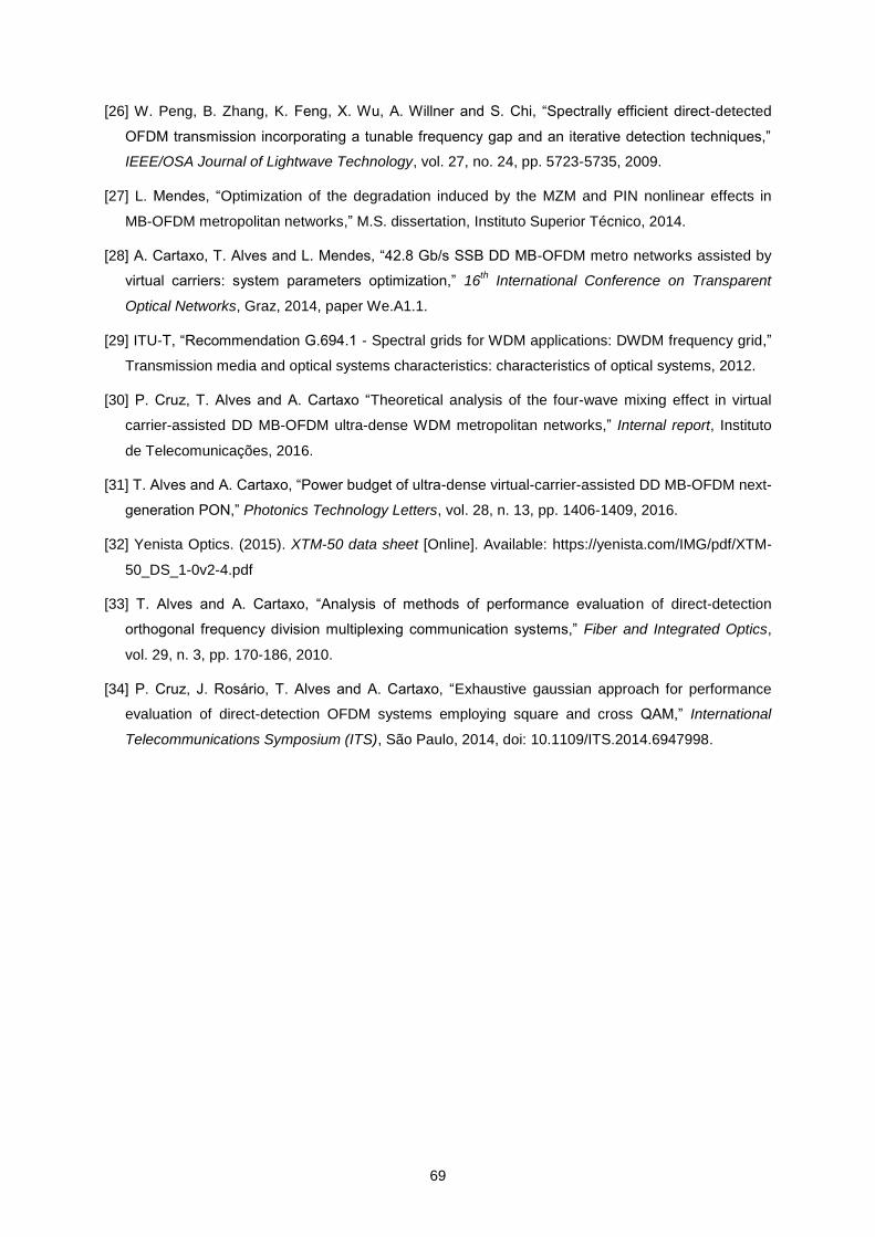
69
[26] W. Peng, B. Zhang, K. Feng, X. Wu, A. Willner and S. Chi, “Spectrally efficient direct-detected
OFDM transmission incorporating a tunable frequency gap and an iterative detection techniques,”
IEEE/OSA Journal of Lightwave Technology, vol. 27, no. 24, pp. 5723-5735, 2009.
[27] L. Mendes, “Optimization of the degradation induced by the MZM and PIN nonlinear effects in
MB-OFDM metropolitan networks,” M.S. dissertation, Instituto Superior Técnico, 2014.
[28] A. Cartaxo, T. Alves and L. Mendes, “42.8 Gb/s SSB DD MB-OFDM metro networks assisted by
virtual carriers: system parameters optimization,” 16th International Conference on Transparent
Optical Networks, Graz, 2014, paper We.A1.1.
[29] ITU-T, “Recommendation G.694.1 - Spectral grids for WDM applications: DWDM frequency grid,”
Transmission media and optical systems characteristics: characteristics of optical systems, 2012.
[30] P. Cruz, T. Alves and A. Cartaxo “Theoretical analysis of the four-wave mixing effect in virtual
carrier-assisted DD MB-OFDM ultra-dense WDM metropolitan networks,” Internal report, Instituto
de Telecomunicações, 2016.
[31] T. Alves and A. Cartaxo, “Power budget of ultra-dense virtual-carrier-assisted DD MB-OFDM next-
generation PON,” Photonics Technology Letters, vol. 28, n. 13, pp. 1406-1409, 2016.
[32] Yenista Optics. (2015). XTM-50 data sheet [Online]. Available: https://yenista.com/IMG/pdf/XTM-
50_DS_1-0v2-4.pdf
[33] T. Alves and A. Cartaxo, “Analysis of methods of performance evaluation of direct-detection
orthogonal frequency division multiplexing communication systems,” Fiber and Integrated Optics,
vol. 29, n. 3, pp. 170-186, 2010.
[34] P. Cruz, J. Rosário, T. Alves and A. Cartaxo, “Exhaustive gaussian approach for performance
evaluation of direct-detection OFDM systems employing square and cross QAM,” International
Telecommunications Symposium (ITS), São Paulo, 2014, doi: 10.1109/ITS.2014.6947998.


71
Appendix A
OFDM system details
A.OFDM system details
In this section we present the transfer function of the single-tap equalizer, as well as some
information regarding the thermal and optical noise.
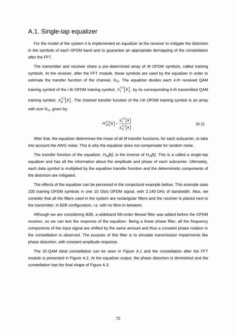
72
A.1. Single-tap equalizer
For the model of the system it is implemented an equalizer at the receiver to mitigate the distortion
in the symbols of each OFDM band and to guarantee an appropriate demapping of the constellation
after the FFT.
The transmitter and receiver share a pre-determined array of M OFDM symbols, called training
symbols. At the receiver, after the FFT module, these symbols are used by the equalizer in order to
estimate the transfer function of the channel, Hch. The equalizer divides each k-th received QAM
training symbol of the i-th OFDM training symbol, i
ts k , by its corresponding k-th transmitted QAM
training symbol, ips k . The channel transfer function of the i-th OFDM training symbol is an array
with size Nsc, given by:
( )
i
tich i
p
s kH k
s k (A.1)
After that, the equalizer determines the mean of all M transfer functions, for each subcarrier, to take
into account the AWG noise. This is why the equalizer does not compensate for random noise.
The transfer function of the equalizer, Heq[k], is the inverse of Hch[k]. This is a called a single-tap
equalizer and has all the information about the amplitude and phase of each subcarrier. Ultimately,
each data symbol is multiplied by the equalizer transfer function and the deterministic components of
the distortion are mitigated.
The effects of the equalizer can be perceived in the conjectural example bellow. This example uses
100 training OFDM symbols in one 10 Gb/s OFDM signal, with 2.140 GHz of bandwidth. Also, we
consider that all the filters used in the system are rectangular filters and the receiver is placed next to
the transmitter, in B2B configuration, i.e. with no fibre in-between.
Although we are considering B2B, a wideband 5th-order Bessel filter was added before the OFDM
receiver, so we can test the response of the equalizer. Being a linear phase filter, all the frequency
components of the input signal are shifted by the same amount and thus a constant phase rotation in
the constellation is observed. The purpose of this filter is to simulate transmission impairments like
phase distortion, with constant amplitude response.
The 32-QAM ideal constellation can be seen in Figure A.1 and the constellation after the FFT
module is presented in Figure A.2. At the equalizer output, the phase distortion is diminished and the
constellation has the final shape of Figure A.3.
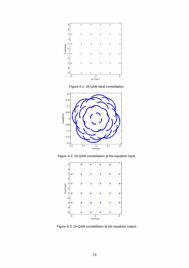
73
Figure A.1: 16-QAM ideal constellation.
Figure A.2: 16-QAM constellation at the equalizer input.
Figure A.3: 16-QAM constellation at the equalizer output.

74
A.2. Electrical noise
At the receiver, there are several components which introduce noise into the signal.
Figure A.4: Equivalent circuit for the front-end.
The front-end of the receiver in Figure A.4 consists of a photodetector, a load resistance RL, and an
amplifier, with noise figure fn and gain g. The resistor introduces noise due to the random motion of
electrons at a finite temperature T, called thermal noise. The thermal noise is additive white Gaussian
noise and its current, iT(t), in the resistor has a variance given by [2]:
2 2 4 BT T T e
L
k Ti t S f df B
R
(A.2)
where Be is the electrical noise bandwidth, and kB is the Boltzmann constant which has the value
1.38×10⁻²³
J/K. The two-sided PSD of the thermal noise current, ST(f), is of the order of 1 (pA)2/Hz.
The amplifier increases the power of the electrical signal but, on the other hand, also amplifies the
noise. Thus, the thermal noise current at the output of the amplifier has a variance of:
2 24 BT e n
L
k TB f g
R (A.3)
Typical values for fn are 3-5 dB.
Finally, the output current is:
out PIN Ti t g i t i t (A.4)
where iPIN(t) is the current at the PIN PD output.
Bias voltage
hν
RL
(fn, g) Output current

75
A.3. Optical noise
The use of OA, with a gain g, has impact in the accumulation of noise, in the form of amplified
spontaneous emission (ASE), which is the spontaneous emission of photons in random directions,
polarisations and phases. The ASE noise, like the optical signal, can be projected in two components,
specifically parallel (∥) and perpendicular (⊥). Also, we consider that the ASE noise power is equally
distributed through all the components, including the in-phase (I) and quadrature (Q) terms. So, the
PSD of the ASE noise of the previous components is characterised by:
, , , , , , , ,4
ASEASE I ASE Q ASE I ASE Q
SS S S S (A.5)
and the ASES is given by:
0 ( 1)ASE nS h f g (A.6)
where h is the Planck constant with the value 6.63×10⁻³⁴
J/Hz. This noise is quantified in terms of the
noise figure fn, usually between 2-5 dB.
Considering a parallel polarisation of the optical signal ,OA ine t , at the output of the OA we get the
signal:
,
, , , , , , , ,Q , , , , ˆˆ
OA out
OA in I OA in Q ASE I ASE ASE I ASE Q ee
e t
e t je t n t jn t n t jn t (A.7)
ASEn t being the ASE noise.


77
Appendix B
Performance evaluation methods
B.Performance evaluation methods
In this section we detail the process to calculate the EVM in the received symbols, as well as the
method used to assess the BER levels, namely the EGA.
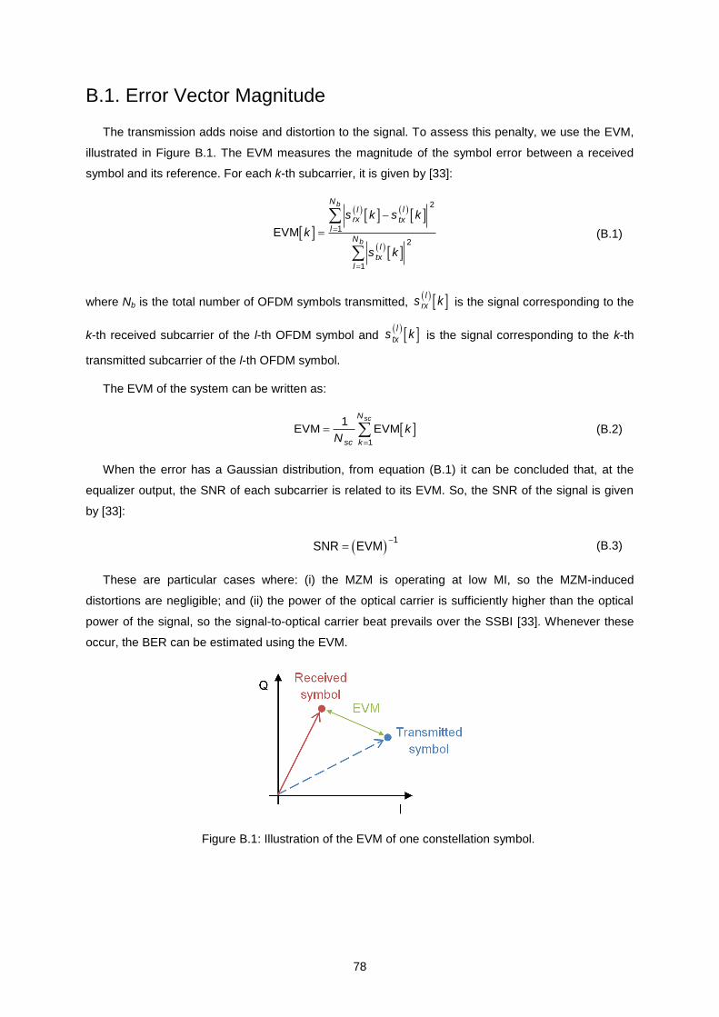
78
B.1. Error Vector Magnitude
The transmission adds noise and distortion to the signal. To assess this penalty, we use the EVM,
illustrated in Figure B.1. The EVM measures the magnitude of the symbol error between a received
symbol and its reference. For each k-th subcarrier, it is given by [33]:
2
1
2
1
EVM
b
b
Nll
rx txl
Nl
txl
s k s k
k
s k
(B.1)
where Nb is the total number of OFDM symbols transmitted, lrxs k is the signal corresponding to the
k-th received subcarrier of the l-th OFDM symbol and l
txs k is the signal corresponding to the k-th
transmitted subcarrier of the l-th OFDM symbol.
The EVM of the system can be written as:
1
1EVM EVM
scN
sc k
kN
(B.2)
When the error has a Gaussian distribution, from equation (B.1) it can be concluded that, at the
equalizer output, the SNR of each subcarrier is related to its EVM. So, the SNR of the signal is given
by [33]:
1
SNR EVM
(B.3)
These are particular cases where: (i) the MZM is operating at low MI, so the MZM-induced
distortions are negligible; and (ii) the power of the optical carrier is sufficiently higher than the optical
power of the signal, so the signal-to-optical carrier beat prevails over the SSBI [33]. Whenever these
occur, the BER can be estimated using the EVM.
Figure B.1: Illustration of the EVM of one constellation symbol.
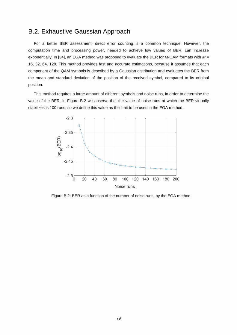
79
B.2. Exhaustive Gaussian Approach
For a better BER assessment, direct error counting is a common technique. However, the
computation time and processing power, needed to achieve low values of BER, can increase
exponentially. In [34], an EGA method was proposed to evaluate the BER for M-QAM formats with M =
16, 32, 64, 128. This method provides fast and accurate estimations, because it assumes that each
component of the QAM symbols is described by a Gaussian distribution and evaluates the BER from
the mean and standard deviation of the position of the received symbol, compared to its original
position.
This method requires a large amount of different symbols and noise runs, in order to determine the
value of the BER. In Figure B.2 we observe that the value of noise runs at which the BER virtually
stabilizes is 100 runs, so we define this value as the limit to be used in the EGA method.
Figure B.2: BER as a function of the number of noise runs, by the EGA method.