Embed Size (px)
Citation preview

3/26/13
1
Composite Variables in SEM Jarre9 E.K. Byrnes
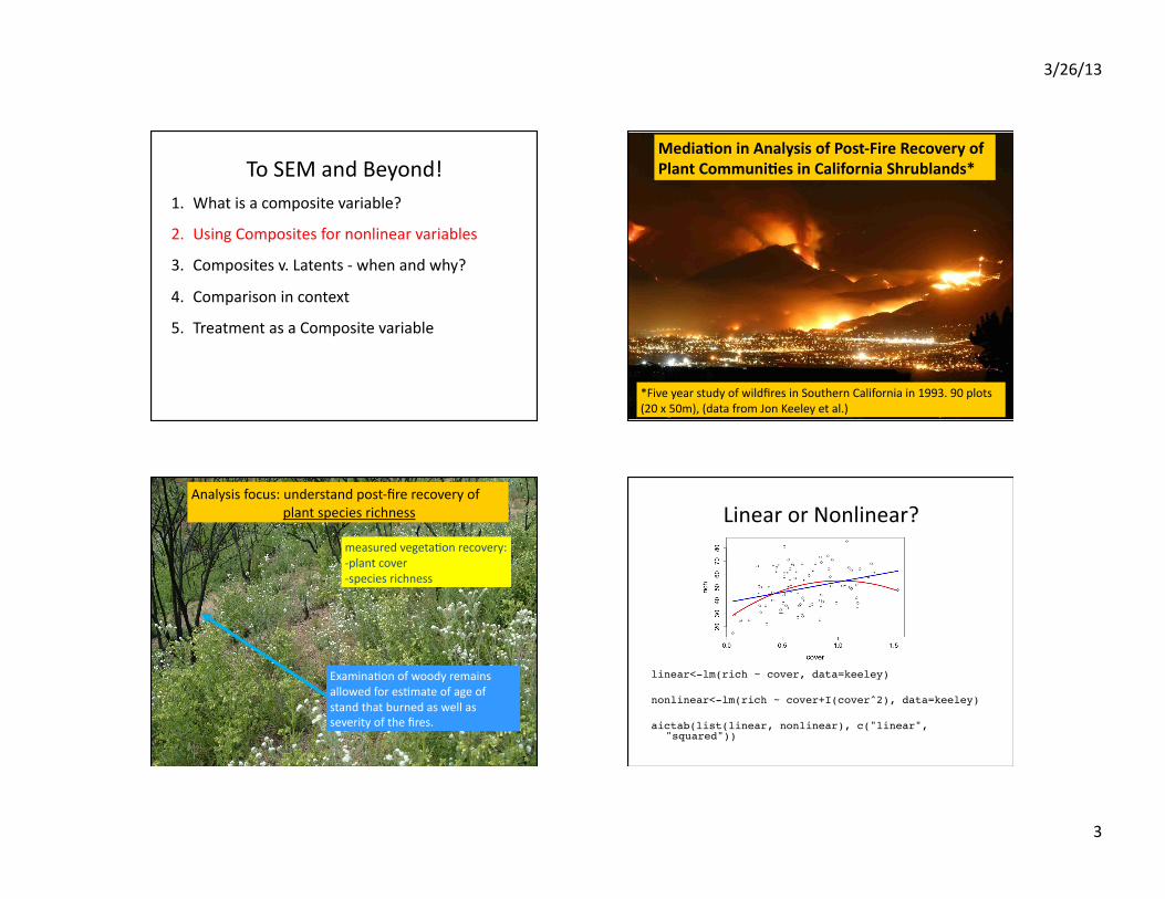
To SEM and Beyond! 1. What is a composite variable?
2. Using Composites for nonlinear variables
3. Composites v. Latents -‐ when and why?
4. Comparison in context
5. Treatment as a Composite variable
We’re Comfortable with Latent Exogenous Variables…
ξ
X1 δx1
X2
X3
δx2
δx3
λx1 λx2
λx3
And Now, Latent Variables Driven by Observed Exogenous Causes
η
X1
X2
X3
λx1 λx2
λx3
ζ
Latent Composite

3/26/13
2
Composite Variables Reflect Joint Effects
X1
X2
X3
λx1
λx2
λx3
0
ηc
• Coefficients can be sta6s6cally es6mated. • Fixing error to 0 aids in iden6fica6on (otherwise it’s a latent composite) • Specifying a scale is oEen helpful.
Coefficients Can be Fixed
Rela6ve Density
Rela6ve Abundance
Rela6ve Frequency
1
1
1
0
Importance Value
Easy way to incorporate concepts into models, par[cularly if exogenous variables have effects beyond the composite variable.
Composites and Nonlineari[es
X
X2
λx
λx^2
0
Indicates one variable derived from another ηc
Composites and Categorical Variables
Nutrient Addi6on
Grazer Addi6on
Fungicide
λx1
λx2
λx3
0
Categories coded as 0 or 1
Treatment
3/26/13
3
To SEM and Beyond! 1. What is a composite variable?
2. Using Composites for nonlinear variables
3. Composites v. Latents -‐ when and why?
4. Comparison in context
5. Treatment as a Composite variable
10
Media6on in Analysis of Post-‐Fire Recovery of Plant Communi6es in California Shrublands*
*Five year study of wildfires in Southern California in 1993. 90 plots (20 x 50m), (data from Jon Keeley et al.)
11
Analysis focus: understand post-‐fire recovery of plant species richness
Examina[on of woody remains allowed for es[mate of age of stand that burned as well as severity of the fires.
measured vegeta[on recovery: -‐ plant cover -‐ species richness
linear<-lm(rich ~ cover, data=keeley)!
nonlinear<-lm(rich ~ cover+I(cover^2), data=keeley)!
aictab(list(linear, nonlinear), c("linear", "squared"))!
Linear or Nonlinear?

3/26/13
4
Model selection based on AICc :!
K AICc Delta_AICc AICcWt Cum.Wt LL!squared 4 735.92 0.00 0.83 0.83 -363.72!linear 3 739.08 3.15 0.17 1.00 -366.40!
Linear or Nonlinear? A Simple Nonlinear Model
#Create a new nonlinear variable in the data!keeley<-within(keeley, coverSQ<-cover^2)!
#Now, for a model!noCompModel <- 'rich ~ cover + coverSQ'!
noCompFit <- sem(noCompModel, data=keeley)!
cover
rich coversq
ζ
A Simple Nonlinear Model
> summary(noCompFit)!…! Estimate Std.err Z-value P(>|z|)!Regressions:! rich ~! cover 57.999 18.613 3.116 0.002! coverSQ -28.577 12.176 -2.347 0.019!
cover rich
R2=0.16 coversq
58.0
-‐28.6
ζ
A Simple Composite Model
compModel<-'!
!! ! ! !coverEffect <~ 58*cover + coverSQ!
!! ! ! rich ~ coverEffect'!
compFit <- sem(compModel, data=keeley)!
rich cover
coversq coverEffect
0
58.0 ζ

3/26/13
5
A Simple Composite Model
Estimate Std.err Z-value P(>|z|)!Composites:! coverEffect <~! cover 58.000! coverSQ -28.577 3.996 -7.152 0.000!
Regressions:! rich ~! coverEffect 1.000 0.321 3.116 0.002!
Variances:! rich 189.597 28.263!
rich R2=0.16
cover
coversq coverEffect
0
-‐28.6
1 58.0
ζ
A Note About the Latent Nature of Composite
• Response variables act like latent variable indicators
• Therefore, responses must share some variance.
• Rules that applied to iden[fiably of latent variables also apply to composites.
• One composite per response if composite error = 0. If composite has mul[ple responses, error variance should be free.
rich cover
coversq coverEffect
0
58.0 ζ
Exercise: A Nonlinear Rela[onship Between abio[c and firesev
Exercise: An Abio[c Composite Model
1. Fit this model – start with a regression
2. Compare the effect of fixing the abiotic loading on abiotic effect to the coefficient from the regression to fixing the abioticEffect on firesev to 1.
firesev abio[c
abio[cSQ abio[cEffect
0
ζ

3/26/13
6
For some reason, this model fails
keeley$abioticSQ <- keeley$abiotic^2!
abioticCompModelBad<-'! abioticEffect <~ 0.4 * abiotic +!!! ! ! ! ! ! ! ! ! ! ! ! abioticSQ!
firesev ~ abioticEffect'!
abioticCompFitBad <- sem(abioticCompModelBad, data=keeley)!
firesev abio[c
abio[cSQ abio[cEffect
0.4
0
ζ
This model does not: try mul[ple methods with composites!
keeley$abioticSQ <- keeley$abiotic^2!
abioticCompModel<-'! abioticEffect <~ abiotic + abioticSQ!
firesev ~ 1*abioticEffect'!
abioticCompFit <- sem(abioticCompModel, data=keeley)!
firesev abio[c
abio[cSQ abio[cEffect 1
0
ζ
Endogenous Composite Variables
endoCompModel<-'! coverEffect <~ 1*cover + coverSQ!
cover ~~ coverSQ! age ~~ coverSQ!
cover ~ age! rich ~ age + coverEffect'!
endoCompFit <- sem(endoCompModel, data=keeley, fixed.x=F)!
rich cover
coversq coverEffect
0
age
δ ζ 1
Endogenous Composite Variables
!! ! ! ! !Estimate Std.err Z-value P(>|z|)!Composites:! coverEffect <~! cover 1.000! coverSQ -0.497 0.078 -6.378 0.000!
Regressions:! cover ~! age -0.002 0.001 -3.129 0.002! rich ~! age -0.201 0.121 -1.667 0.095! coverEffect 48.705 19.246 2.531 0.011!
rich cover
coversq coverEffect
1
0
age
δ ζ
48.7
-‐0.20
-‐0.49

3/26/13
7
To SEM and Beyond! 1. What is a composite variable?
2. Using Composites for nonlinear variables
3. Composites v. Latents -‐ when and why?
4. Comparison in context
5. Treatment as a Composite variable
Consider This Model…
Urchin Grazing
Nutrient Availability
Giant Kelp
Purple Urchins
Red Urchins
Mean Temperature
# Days of Low Nutrients
Giant Kelp Observed
ε1 ε2
ζ2
δ1 δ2
ζ1
(1)
(1) (1)
0.24
Urchin Grazing
Nutrient Availability
Giant Kelp
Purple Urchins
Red Urchins
Mean Temperature
# Days of Low Nutrients
Giant Kelp Observed
ε1 ε2 δ1 δ2
ζ1
(1)
(1) (1)
What is the direc[on of causality?
ζ2 0.24
What is the direc[on of causality?
Nutrient Availability
Giant Kelp
Purple Urchins
Red Urchins
Mean Temperature
# Days of Low Nutrients
Giant Kelp Observed
ε1 ε2 δ1 δ2
0
(1)
(1) (1)
Grazing Pressure
ζ2 0.24

3/26/13
8
Are the indicators in a block interchangeable?
Nutrient Availability
Giant Kelp
Purple Urchins
Red Urchins
Mean Temperature
# Days of Low Nutrients
Giant Kelp Observed
ε1 ε2 δ1 δ2
0
(1)
(1) (1)
Grazing Pressure
Correla[on=0.78
ζ2 0.24
Do indicators covary because of joint causes?
Nutrient Availability
Giant Kelp
Purple Urchins
Red Urchins
Mean Temperature
# Days of Low Nutrients
Giant Kelp Observed
ε1 ε2 δ1 δ2
0
(1)
(1) (1)
Grazing Pressure
YES! Temperature!
ζ2 0.24
Do indicators have a consistent set of causal influences?
Nutrient Availability
Giant Kelp
Purple Urchins
Red Urchins
Mean Temperature
# Days of Low Nutrients
Giant Kelp Observed
ε1 ε2 δ1 δ2
0
(1)
(1) (1)
Grazing Pressure
YES! Currents!
ζ2 0.24
Latents and Composites Together: L-‐C Block for Measurement Error
Grazing Pressure
δ1
δ2
δ3
Red Urchin Density
Measured Red Urchin Density
Measured Purple Urchin Density
Measured White Urchin Density
Purple Urchin Density
0
White Urchin Density
3/26/13
9
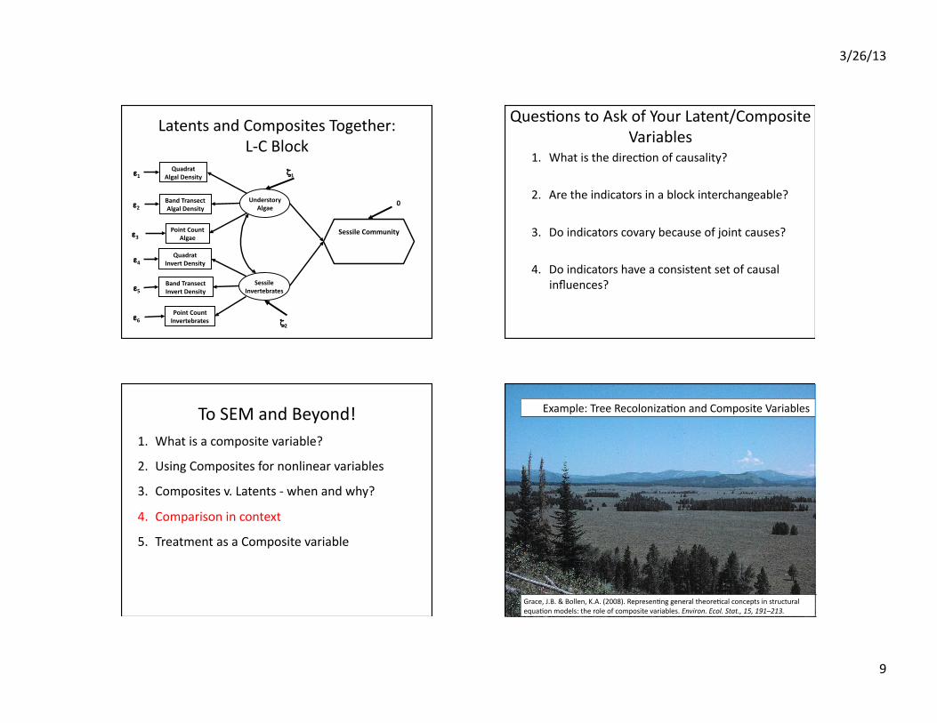
Latents and Composites Together: L-‐C Block
Sessile Community
ε1
ε2
ε3
Understory Algae
Quadrat Algal Density
Band Transect Algal Density
Point Count Algae
ζ1
Sessile Invertebrates
Quadrat Invert Density
Band Transect Invert Density
Point Count Invertebrates
ε4
ε5
ε6 ζ2
0
Ques[ons to Ask of Your Latent/Composite Variables
1. What is the direc[on of causality?
2. Are the indicators in a block interchangeable?
3. Do indicators covary because of joint causes?
4. Do indicators have a consistent set of causal influences?
To SEM and Beyond! 1. What is a composite variable?
2. Using Composites for nonlinear variables
3. Composites v. Latents -‐ when and why?
4. Comparison in context
5. Treatment as a Composite variable
Grace, J.B. & Bollen, K.A. (2008). Represen[ng general theore[cal concepts in structural equa[on models: the role of composite variables. Environ. Ecol. Stat., 15, 191–213.
Example: Tree Recoloniza[on and Composite Variables

3/26/13
10
What is the Contribu[on of Local versus Regional Factors to Recoloniza[on
Grace and Bollen 2008
Adding Variables to the Metamodel
Grace and Bollen 2008
Latent or Composites?
Grace and Bollen 2008
What do you think?
Generality v. Specificity
Grace and Bollen 2008

3/26/13
11
Generality v. Specificity
Grace and Bollen 2008
χ2=45.20 DF=10 P<0.00005
χ2=6.88 DF=3 P=0.075
How Confident are We in Composite Loadings and their Conclusions?
Specific model without composites provides similar answers.
Tes[ng our Confidence in Composites
The general composite construct is not obscuring more specific rela[onships in the data.
To SEM and Beyond! 1. What is a composite variable?
2. Using Composites for nonlinear variables
3. Composites v. Latents -‐ when and why?
4. Comparison in context
5. Treatment as a Composite variable

3/26/13
12
Previous Model Unstandardized
1. Rhodymenia is not good food. – Urchins eat more, but produce less gonad
2. Performance is similar with Macrocystis or Mixture diet
MAPY
Feeding.rate.dry GONAD_INDEX
R
0.67 0.38
0.002 -‐0.57
Treatment as a Composite Affec[ng Mul[ple Responses
#read in and binary-ize the treatment!urchinData<-read.csv("./urchin_ex_sem.csv")!source("./makeBinaryTreatments.R")!
binTrt<-makeBinaryTreatments(urchinData, "treatment")!
urchinData<-cbind(urchinData, binTrt)!
MAPY
Feeding.rate.dry GONAD_INDEX
R
ζ3 ζ
Treatment 0
A Composite Treatment Model
urchinCompositeModel<-' !!Treatment <~ MAPY + .002*R!
Feeding.rate.dry ~ Treatment! GONAD_INDEX ~Treatment + Feeding.rate.dry!'!
MAPY
Feeding.rate.dry GONAD_INDEX
R
ζ3 ζ
Treatment
0.002
0
MAPY Has No Effect
lavaan (0.5-12) converged normally after 71 iterations!
Used Total! Number of observations 20 21!
Estimator ML! Minimum Function Test Statistic 1.993! Degrees of freedom 1! P-value (Chi-square) 0.158!
MAPY
Feeding.rate.dry GONAD_INDEX
R
0.72 0.39
Treatment
0.002
0
1.05 -‐19.94
Composite reflects R

3/26/13
13
Exercise: Fit this Model
> urchinCompositeFit2<-sem(urchinCompositeModel2, data=urchinData)!Error in solve.default(E) : ! system is computationally singular: reciprocal condition number =
2.09555e-16!
[lavaan message:] could not compute standard errors!!
You can still request a summary of the fit to inspect! the current estimates of the parameters.!
MAPY
Feeding.rate.dry TEST_CHANGE
R
ζ3 ζ
Treatment
0.002
0
SCALE PROBLEM
Exercise: Fit this Model
> head(urchinData[,c(5,17)])! Feeding.rate.dry TEST_CHANGE!1 0.006454893 7.68!2 0.011449023 3.74!3 0.012258490 5.78!4 0.007628933 6.34!5 0.011282345 5.00!6 0.007344447 4.94!
MAPY
Feeding.Rate.dry
R
ζ3 ζ
Treatment
0.002
0
TEST_CHANGE
Transform Scales to Fit
urchinData$TEST_CHANGE_10<-!!! ! !urchinData$TEST_CHANGE/10!
MAPY
Feeding.rate.dry
R
ζ3 ζ
Treatment
0.002
0
TEST_CHANGE
Fit Model
!! ! ! ! ! Estimate Std.err Z-value P(>|z|)!
Regressions:! Feeding.rate.dry ~! Treatment 0.888 0.319 2.785 0.005! TEST_CHANGE_10 ~! Treatment -104.771 32.011 -3.273 0.001! Feedng.rt.dry 23.670 16.784 1.410 0.158!
MAPY
Feeding.Rate.dry
R
ζ3 ζ
Treatment
0.002
0
TEST_CHANGE_10
-‐104.7 23.7

3/26/13
14
A Composite Conclusion
• Composite variables are useful as variables to gather informa[on about mul[ple aspects of a single effect.
• Excellent for represen[ng nonlineari[es.
• Oten what ecologists think of in terms of aggregate variables.
• Provide method of incorpora[ng complex treatment effects.