10 C-AKkc, IN - MIT OpenCourseWare · Solve the conduction equation in radial coordinates, in 1D, with heat generation, and apply the boundary conditions

1. ~ ~ k ~ 10 C-AKkc, = k IN 'OA:~AL V'Ll\f~'t:.

III :::- k \ \ -ro (- (>><'15

k II :: I, s 3 -7!f'i.- 3mk. ~ kll =o· o() 50 p 3k...'A.T

r-l'r" '\N IiI.!, if'>.. \...-11'i§"'?-- -------'--------1 -[k:T~~ :::- (0. 00 6\ 3 01~~)' - (c, 001*1 ~)

--""..."'-~.-,----.--...-.......--.~,-"'..~~~..-. --"",,~.. --.

D \ "'~S f.~1\j;T p,.-r X 2> j., +b)l. I TI.k N Ky IS A ftJNC7!oN

b , 6. k~,(\N\(>L) ();l-'1 ) Ot '/.. / foo, 'S,cM £- rOY<...

( \. f. / UN£A.R.L'1 f4f'f'R..6)<.1 MA If. K", 't;'l: ) USc A ~'tLO?- S£R-I-&'S

\-r \s J'~f S A/I/\E F<5¥?- k't &. \<: l .LE'1 IS DO l-r 'fa?2._ k",·

6.'f.. ' - k dk", Jk ::::\<. +J.kx - x+~ x.ASSOM£: )<.+AX X 0 r

"\~ E- N \;J ~ tl ~v£ ( vJi<JII N6j lx Ix -- k>< '):

-(kx~ Ix -&, +-~~ ox) !: \,-",,~ ') ---'-------.;:::,-'X,---.---.....--......-----:»

"dk ciTrk~~C:,,=-k ~t) + dXx

6X~ )(:tl ..

~~ loX

~ kx~ \,+"~- !:\J .1::.)'..

p2

No'fJ / ""t: CA \. L. -r:~ E

~ 1-~ 1-= £ d~ C>'A J J d ><.

~I2.AP\J\ -r-E)

k.'i ~. KJ.

l<-E-$IS ~Lf.) o~ SAu4 fAI"(p NJ> Po. 'Lf, .on.. f/?..J"'-A L

S E f \ f- \j'J t (AN NE~ lE CI'c:;iF DIe..e(::(I~S -\"o

p,. .D I f.b...f; N .s IOI"J ' k...

k.L iZ,,, K..L 11<.11 kJ. R.'1-- -L-l. '«..'>( L.L. - - ------ ='1 . R.t -- -

-. R

2.

I.;... 1<.1\ Lj./ LI/ ~llR'I ..-. - ) 1.-" 'L.-J!L. EQ"I> I.

\s IN -n.\f rt.ANL:lj E. 0,1.L.. P..A-rtcr .( 10 • \y::: ~\IO

~12-&E: f..,A-no S / yo#- AL-L-CA,NNO"'- Nf:C\ LEe-r AN"! DIR.ECl''tcJ'f\lS/.

\116N WE p~U;M \S 3D.

~N.D I\~E:. ., , I·j ..

\{ . oN€"" {?...A-rla \s avrSIDE TW IS tf..AI\i(;,E/ TI~ErJ •

\~.E. Pl2..c/?)LfM. \S 5TI/.-L 3D

( f.1.q . I f .~ \tJ £f-C N.fqU 6t IME / -n-J r':N

!0:.iLt SilL-I.- INV61--\lS D) ~ND ItJAT INGLl)OES AI-\.. 3 f2..-E- S I -rr"N c.E-S0

• If L ~ICiS A~ ()IITslDE f1-J IS

\l-l£ 'PeJ6I-'t: M \S 2D.

~ It ~L--L- ~ \2.Afl0..s AP~E. oUTSIDE. -n.\l~ ~lE,/ \i~t:N "NL'-I {\J{ SLr..)w fS I"" DiR.EC-rlaN fY\...Arff:R..5I b.ND I~t Ptf~l€-M \ S --iO.

(, . 1Zx. IZL .)d I -- .-- -

--,- 1 j So

R~ Kl.

CJ::.N N~vEK \JIWE. A ~D

f2...'K R,/ 7 •R-:t:.::::: f.2.l=. =

PLI) ~ \ t'i ( ae._ «..J.-n 01 :

(0, 14 2~1-) T - (Cl,-=t (~-~)

( i'l ," as', ~~)T - (0, o04fCj~ \",,",-- )

'Tt.I \ 'S > \ 0 OK <:. 0 \ \ 'W r-\£N IS

USI"J S N\.~'n..le/IA..AJ\ cA J vJE FI N () TI..JAJ

-rIO == 3.13 K 3.. T:','~::: 2Qs K I OAT I

_ 10 ---r ~, 6xC£EOS \0 ,l \l EO l"-I'"TiOlc.R-t-r J

sP I y.,t·E 'rl f".,.,j f --n~ t>. -r ~ yOlZ. I ~ 3,"2-) \(!

C-AX/S

LooKI NG AI' -nJ1'S SLICE:

o C-AXIS

~ Ho'"f-reJ2..

• ::::'\-1 o '"fiE'S I

\-1\qU-SR- IN IN& 8A:S,4.L.- PL-ANG. ,&E;cA0~E; THE A1oi'l\S

IN -(\..\£ 6~<AL.- PLANe AK£. c.oVAl...Gl\lil'i e,aN.Dl:;D. j;*fSE

SirC...6N{q I ~M"tl..'1 ,BoNDS ALl-OW FCllt.. \!€.tZ.'f t:.FF.!<:yENT

coLJPI.AN!:j Of ~-roMI'- AND ~L..f~f,t..6Ntc.. VII';,ItA'f'I()'f\jS•

\"12..ANS,ftj12..:i ALJ:;Nq Ti4€. c...,-Ax.l S IS ESP £0 AvL'1 PooP,

Uc.Au<)£ '"'11jf.. !3oNDS IN -r1-l 15 DIIZ.EG1I~ A,P.,£

v.)£A't:.. VfY'J r£~ vv'At.L.S \i\JTh~c..l1aNS.

--

Ai = ~L7Lr

AL == 271. {r+t::..r') V -::::: /f(r-+ /;:" r- -7[ r 2..

-~2~:'~~') ~~ r + k~:~:d *n.: t =~ fe f

0Nc£-~-r--.

\ S sfVJ::> L-L !

~rV- is N ~q \-\(;'1 16 LI<:

~~ \ U~ t r;.r :'~

---------------~

\,\0\ Ie,

. ------- IF" = Z-S"'C<=t

j~Q'0NDJ:\e'1 C9ND1"f\6NS ~

.1- \TiS (2...C£) \ S AAOIALL'1

S'-l0--fV'\citZ-IC'1 ~ ~T

y- :::. 0 / Sl::::. 0 d'

2. p-,-r \.lE- 'S.[)R.-~IK:EJ T~G~f 6N\S CoN\J£Cil . dl \ _ ( )

_ ,() - \<. - - h Ts- 1;1-1"--./ 2Jr

, f-. INh ~ I0 ~ "::iJR. t:,,1R...

i. n\ .:=0: ~r

r= 0

•• •

I. ::::;, -t- T(=

.-.f[....L)~ IN \-6'J2... \5 "10

Ts T \ ,~~ :c;: --_._

._--_.._-----,-

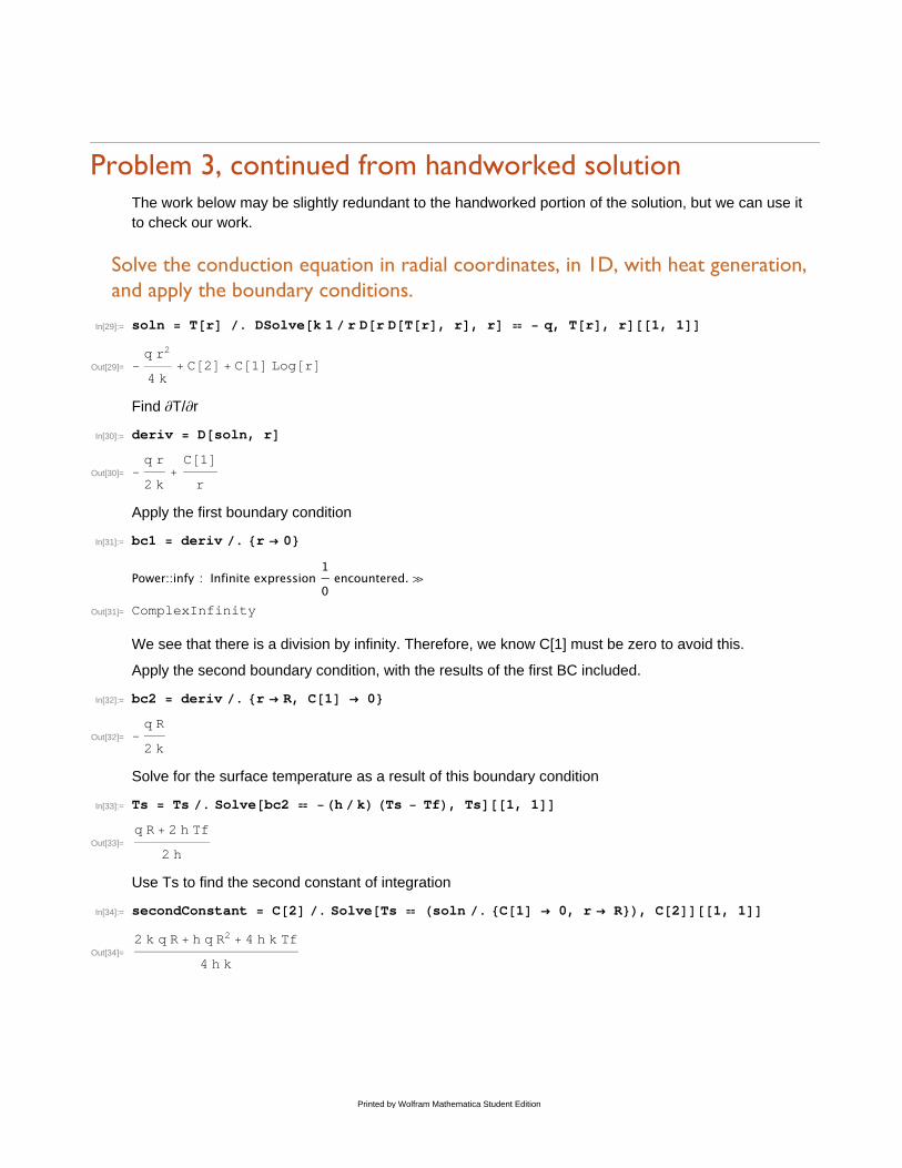
Problem 3, continued from handworked solution The work below may be slightly redundant to the handworked portion of the solution, but we can use it to check our work.

Solve the conduction equation in radial coordinates, in 1D, with heat generation, and apply the boundary conditions.

In[29]:= soln = T@rD ê. DSolve@k 1 ê r D@r D@T@rD, rD, rD ã - q, T@rD, rD@@1, 1DD

q r2

Out[29]= - + C@2D + C@1D Log@rD 4 k

Find !T/!r

In[30]:= deriv = D@soln, rD

q r C@1D Out[30]= - +

2 k r

Apply the first boundary condition

In[31]:= bc1 = deriv ê. 8r Ø 0<

Power::infy : Infinite expression encountered. à 0

Out[31]= ComplexInfinity

We see that there is a division by infinity. Therefore, we know C[1] must be zero to avoid this.

Apply the second boundary condition, with the results of the first BC included.

In[32]:= bc2 = deriv ê. 8r Ø R, C@1D Ø 0<

q R Out[32]= -

2 k

Solve for the surface temperature as a result of this boundary condition

In[33]:= Ts = Ts ê. Solve@bc2 ã -Hh ê kL HTs - TfL, TsD@@1, 1DD

q R + 2 h Tf Out[33]=

2 h

Use Ts to find the second constant of integration

In[34]:= secondConstant = C@2D ê. Solve@Ts ã Hsoln ê. 8C@1D Ø 0, r Ø R<L, C@2DD@@1, 1DD

2 k q R + h q R2 + 4 h k Tf Out[34]=

4 h k

1

Printed by Wolfram Mathematica Student Edition

2

In[35]:= Expand@secondConstantD

q R q R2

Out[35]= + + Tf 2 h 4 k

This agrees with our work by hand. The full solution is therefore:

In[36]:= temperature = soln ê. 8C@1D Ø 0, C@2D Ø secondConstant<

q r2 2 k q R + h q R2 + 4 h k Tf Out[36]= - +

4 k 4 h k

Visualize the solution with real numbers: k = 27.5 W êmK

h = 10 W ëm2 K

R = 0.125 m Tf = 298 K

3r = 1730 kgëm

cp = 27.665 J/mol K times 1/0.238 mol/kg

3We don’t know what the heat production production rate will need to be, so let it be set to 10x W ëm , and we’ll use a slider to vary x.

Out[50]=

Log@q ° D

3.3

0.05 0.10 0.15 0.20 0.25r @mD

300

305

310

THrL @KDTemperature in the rod & surrounding air

Wow! The thermal profile is really flat. Let’s look closely for q = 104 W ëm3:


= 7.0 109 molëm3

Since there are only ~7270 molëm3for uranium, there is no risk of overheating the rod. We haveassumed that 100% of the energy released by the decay is heat, but even if this is way off, it will notchange our answer by 5 orders of magnitude. Of course, rods can overheat in real life and cause a melt-down, but that is because neutrons released in radioactive decay can catalyze other nuclei to decayand set off a chain reaction. We have completely neglected this chain reaction effect here, but it essen-tial for nuclear power plants to work - without this effect, fission would not release nearly enough heat tobe a useful source of energy (as is shown by our analysis here).

3

Temperature in the rod for q = 104 Wêm3

THrL @KD

361.8

361.6

361.4Out[38]=

361.2

361.0

360.8

360.6

r @mD0.02 0.04 0.06 0.08 0.10 0.12

The profile is sloped, but only very slightly. I’d bet the Biot number is really small...

Find the maximum allowable rate of heat production.

Set the tempearture equation equal to 660 C:

In[39]:= maxQ = q ê. Solve@temperature ã 660 + 273, qD@@1, 1DD

4 h k H-933 + TfL Out[39]= -

-h r2 + 2 k R + h R2

Plug in real numbers for uranium in air:

In[40]:= maxQrealNumbers = maxQ ê. 9k Ø 27.5, h Ø 10, R Ø 0.125, Tf Ø 298,

rcp Ø I1730 H*kgëm3*L 27.665 H*Jêmol K*L 0.238-1 H*molêkg*LM=

698 500. Out[40]=

7.03125 - 10 r2

This still depends on r. But, we realize that the hottest point in the rod ought to be the point fatherest from the edges, r = 0. So, plug this in as well:

In[41]:= maxQ = maxQrealNumbers ê. r Ø 0

Out[41]= 99 342.2

3In summary, we find that the heat production in the rod may not exceed 99000 W ëm .

Out of curiosity, what concentration of U-235 (i.e., enrichment), which is the most radioactive isotope of uranium, must there be in the rod to achieve this heat production rate?

If you are curious, you can derive this expression assuming exponential radioactive decay (it is not difficult, but could be fun) t1ê2 = 704 million years and the energy released per decay is 4.679 MeV:

N0 = q t1ê2 / Ln2 DE

= ((99000 J ês m3M (704 106 yr) (3.156 107 sec/yr)) / (Ln2 (4.679 MeV) (1.602 10-13 J/MeV))

m -3 = 4.2 1033


In summary, we find that the heat production in the rod may not exceed 99000 W ëm3.

Out of curiosity, what concentration of U-235 (i.e., enrichment), which is the most radioactive isotope ofuranium, must there be in the rod to achieve this heat production rate?

If you are curious, you can derive this expression assuming exponential radioactive decay (it is notdifficult, but could be fun)t1ê2 = 704 million years and the energy released per decay is 4.679 MeV:

N0 = q t1ê2 / Ln2 DE

= ((99000 J ês m3M (704 106 yr) (3.156 107 sec/yr)) / (Ln2 (4.679 MeV) (1.602 10-13 J/MeV))

= 4.2 1033 m-3

°°

°

Problem 5: determine the dominant heat transfer process,i.e., the rate-limiting step

4

3 = 7.0 109 molëm

Since there are only ~7270 molëm3for uranium, there is no risk of overheating the rod. We have assumed that 100% of the energy released by the decay is heat, but even if this is way off, it will not change our answer by 5 orders of magnitude. Of course, rods can overheat in real life and cause a melt-down, but that is because neutrons released in radioactive decay can catalyze other nuclei to decay and set off a chain reaction. We have completely neglected this chain reaction effect here, but it essen-tial for nuclear power plants to work - without this effect, fission would not release nearly enough heat to be a useful source of energy (as is shown by our analysis here).

Problem 4

Repeat the analysis using the Biot number

I decided to change the statement of this problem after I initially wrote it, and thus it was necessary to use h = 2 W ëm2K to ensure that we were in the Newtonian regime. But, it turns out that this was unness-esay - we can see from our plots above that we are well within the Newtonian regime even in air. So, lowering h will not change out answer - it is Newtonian either way! Let’s prove it:

Bi = h L / k = (10 W ëm2 K) (0.125 m) / (2 27.5 W/mK) = 0.023 with h = 10 W ëm2K

and Bi = 0.0045 with h = 2 W ëm2K.

In either case, conduction is really fast and there are no temperature gradients. Thus, we can say at steady state, the rate of heat accumulation is zero:

rate of accumulation = A qin - A qout + V qgen = 0 where A is the area through which heat is lost/gained, and V is the volume over which heat is generated. qin = 0, so A qout = V qgen

h HTss - Tf) (2 p R z) = q (p R2 z) 2 h HTss - Tf) = q R

2 h HTss - TfL q = R

This equation relates the steady-state temperature with the rate of heat production in the rod. Much easier!

If Tss may not exceed 660 C and h = 2 W ëm2 K, then the maximum rate of heat production allowed is

2.0 104 W ëm3. Using this model and h = 10 W ëm2 K to check our previous work, we find the maxi-

mum rate of heat production is 102 000 W ëm3, which is extremely close to the actual value of 99000 3W ëm .


4. Convection of the aggitated air at the water surface

Note: The thermal conductivity of water is ~0.6 W/mK (from NIST: http://www.nist.gov/data/PDF-files/jpcrd493.pdf). The thermal conductivity of plastics and fibers is usually between ~0.2 - 1 W/mK, solet’s pick ~0.6 for hair. The air is highly aggitated, so h ~50 W ëm2 K.

Next, make relevant comparisons of the rates of heat transfer:

Compare 2 & 3: Is water better at conducting, or convecting? The water is probably nearly stagnant(though agitated vs. stagnant doesn’t matter much), so let’s pick h = 1400 W ëm2K. Convective conduc-tivity = h. Conductive conductivity = k/L. Thus, the comparison is h L/k, like a Biot number, except the kvalue is also for the fluid. h L/k = 0.093, so we can probably neglect the convection and only worryabout water conduction. Note that convection is usually faster than conduction in water, but we are inthe unusual case of a very, very thin layer of water, so conduction actually wins out.

Compare 1 & 2: The length to use for the hair is R/2 = 20mm. The length to use for the water is 40mmbecause it is a one-sided heat transfer (ignoring the cylindrical nature of the geometry). The ratio ofconductivities is Hk êLLwater ê Hk êLLhair = 0.5. Thus, conduction is equally important in the hair and water. Infact, because their thermal conductivities are equal, they act like one uniform material with radius R =80mm. This approximation works because convection only contributes a little to the heat transfer.

Compare 1/2 & 4: Use the Biot number to compare conduction through the strand/water layer andconvection in air. h L/k = (50 W ëm2 K) (40 mm) / (0.6 W/mK) = 0.0033, thus conduction in the solid/liq-uid is fast and transfer from the air is limiting.

Finally, decide what matters, and doesn’t matter:This case afforded us some nice simplifications, and one process clearly emerged as limiting. Heattransfer via convection from the air to the surface of the wet hair strand is rate-limiting.

5

Problem 5: determine the dominant heat transfer process, i.e., the rate-limiting step

Cooling a 1m wide, 0.4m thick billet of steel in a 1m thick refractory mold, open on top

First, list all of the heat transfer processes happening: 1. Conduction inside the steel 2. Conduction to the mold on 4 equivalent sides (the 1m direction) 3. Conduction t the mold through the bottom (the 0.4m direction) 3. Convection on the top of the billet

Note: The thermal conductivity of steel is ~37 W/mK. The thermal conductivity of a typical refractory blend is about 5-10ish W/mK near the 1000K, so let’s pick 8 W/mK.


Compare 1 & 2: The length to use for the steel is 0.5m because heat is escaping on both sides, i.e., it only has to cross half of the billet to escape. The length to use for the mold is 1m because it is a one-sided heat transfer. The ratio of conductivities is Hk êLLmold ê Hk êLLsteel = 0.11. Thus, conduction in the steel is faster than through the mold, but not by a whole lot.

Compare 1 & 3: This is just like before, except the length for the steel is 0.2m. The ratio of conductivities is Hk êLLmold ê Hk êLLsteel = 0.043. Thus, we know conduction in the steel is fast, and this is not limiting.

Compare 3 & 4: Use the Biot number, h L/k = (10 W ëm2 K) (0.2 m) / (37 W/mK) = 0.054, thus conduc-tion in the steel is fast and loss to the air is limiting.

Finally, decide what matters, and doesn’t matter: Because the billet is thin in one dimension, and conduction along that dimension to the air and mold is fast compared to convection in air and conduction in the mold, we can neglect conduction within the billet. If the ratio of conductivities was more extreme in the 1 & 2 comparison, we might have to worry about conduction within the plane of the billet as well, but it is 0.11, which is only barely over our factor-of-10 cut off. However, the ratios when comparing 1 & 2, 1 & 3, and 3 & 4 are very similar: 0.043/0.054 = 0.80; 0.11/0.054 = 2.0; 0.11/0.043 = 2.6. They are all silimar. This means that the rate-limiting heat transfer process is loss of heat from the billet to the surroundings: tranfer processes 2, 3, and 4 are all important, only process 1 can be neglected.

Blow-drying wet hair

First, list all of the heat transfer processes happening: 1. Conduction inside the hair strand 2. Conduction through the water layer 3. Convection within the water layer


First, list all of the heat transfer processes happening:1. Conduction inside the hair strand2. Conduction through the water layer3. Convection within the water la r

Finally, decide what matters, and doesn’t matter:Heat transfer via convection of the water at the copper surface is rate-limiting.

6

ye 4. Convection of the aggitated air at the water surface

Note: The thermal conductivity of water is ~0.6 W/mK (from NIST: http://www.nist.gov/data/PDF-files/jpcrd493.pdf). The thermal conductivity of plastics and fibers is usually between ~0.2 - 1 W/mK, so let’s pick ~0.6 for hair. The air is highly aggitated, so h ~50 W ëm2 K.


Compare 2 & 3: Is water better at conducting, or convecting? The water is probably nearly stagnant (though agitated vs. stagnant doesn’t matter much), so let’s pick h = 1400 W ëm2K. Convective conduc-tivity = h. Conductive conductivity = k/L. Thus, the comparison is h L/k, like a Biot number, except the k value is also for the fluid. h L/k = 0.093, so we can probably neglect the convection and only worry about water conduction. Note that convection is usually faster than conduction in water, but we are in the unusual case of a very, very thin layer of water, so conduction actually wins out.

Compare 1 & 2: The length to use for the hair is R/2 = 20mm. The length to use for the water is 40mm because it is a one-sided heat transfer (ignoring the cylindrical nature of the geometry). The ratio of conductivities is Hk êLLwater ê Hk êLLhair = 0.5. Thus, conduction is equally important in the hair and water. In fact, because their thermal conductivities are equal, they act like one uniform material with radius R = 80mm. This approximation works because convection only contributes a little to the heat transfer.

Compare 1/2 & 4: Use the Biot number to compare conduction through the strand/water layer and convection in air. h L/k = (50 W ëm2 K) (40 mm) / (0.6 W/mK) = 0.0033, thus conduction in the solid/liq-uid is fast and transfer from the air is limiting.

Finally, decide what matters, and doesn’t matter: This case afforded us some nice simplifications, and one process clearly emerged as limiting. Heat transfer via convection from the air to the surface of the wet hair strand is rate-limiting.

Quenching oxidized copper in water

First, list all of the heat transfer processes happening: 1. Conduction inside the copper 2. Conduction through the oxide layer 3. Convection of the water

Note: The thermal conductivity of copper is ~390 W/mK. The thermal conductivity of copper oxide isn’t provided in our tables, but all oxides are about 5-10ish W/mK, so let’s pick 8 W/mK.


Compare 1 & 2: This is a two-sided sheet, so LCu = 1.5cm and Loxide = 10 mm. Hk êLLCu ê Hk êLLoxide = 0.033. Thus, we can neglect the oxide layer because it does not sustain temperature gradients.

Compare 1 & 3: Compute the Biot number for stagnant water: h L/k = (10 W ëm2 K) (0.015 m) / (390 W/mK) = 0.00038. Thus, conduction is waaay faster than convection.


http://www.nist.gov/data/PDF

First, list all of the heat transfer processes happening:1. Conduction inside the copper2. Conduction through the oxide layer3. Convection of the water

Note: The thermal conductivity of copper is ~390 W/mK. The thermal conductivity of copper oxide isn’tprovided in our tables, but all oxides are about 5-10ish W/mK, so let’s pick 8 W/mK.


Compare 1 & 2: This is a two-sided sheet, so LCu = 1.5cm and Loxide = 10 mm. Hk êLLCu ê Hk êLLoxide =0.033. Thus, we can neglect the oxide layer because it does not sustain temperature gradients.

Compare 1 & 3: Compute the Biot number for stagnant water: h L/k = (10 W ëm2 K) (0.015 m) / (390W/mK) = 0.00038. Thus, conduction is waaay faster than convection.

7

Finally, decide what matters, and doesn’t matter: Heat transfer via convection of the water at the copper surface is rate-limiting.

Quenching oxidized copper in water

First, list all of the heat transfer processes happening: 1. Conduction inside the polyester 2. Convection of the air around the powder 3. Conduction of heat through the aluminum into the polyester

The aluminum substrate can in theory contribute heat to the powder particles, but the contact area is very small. If you chose to neglect transfer via aluminum, that is okay.

Note: The thermal conductivity of aluminum is ~235 W/mK. The thermal conductivity of polyester (a typical polyester is PET) is ~0.2 W/mK.


Compare 1 & 2: Compute the Biot number: h L/k = (10 W ëm2 K) (16.7 mm) / (0.2 W/mK) = 0.00084. Thus, conduction is much faster than convection.

Compare 2 & 3: Compute the Biot number: h L/k = (10 W ëm2 K) (0.0015 m) / (235 W/mK) = 0.000064. Thus, conduction is much faster than convection.

Compare 1 & 3: Heat reaches the aluminum on both sides, so LAl = 1.5mm and Lpowder = R/3 = 16.7 mm. Hk êLLAl ëHk êLLpowder = 13. Thus, the aluminum heats up quickly compared to the powder, so it is possible that the main source of heating is actually via the contact with the substrate (especially for real particles, which are not spherical).

Finally, decide what matters, and doesn’t matter: The most likely way the particles heat up is by the air heating the aluminum, which heats the powder particles from below. Thus, the limiting heat transfer process is convective transfer from the air to the aluminum.


Co.

-de

~ == i ~ coS(k~) + ~ S\N(k~)100 d L

.s§:: ~ -~A/t")9N(l~) + K ~I<.(L) co~(kS) d~ r..~O

'"i':f',. ":t - Ie'- A/c) '-"" /'3) - \<."- ,,/1::) S'N (k~) d :::> 1<:-0

- _ k1. 6(\/C)

S I) e:,<;1'11" I.,)"T (; e \!\lId 1-\ ~i:I\e:-~ Vi"--naN:

fo ~ 'd.>\<.~ -r ~~ S'N k~ = ~o-k'1. /.\/e) Co; \:~ _k'2 5/r)'" KJ

p.,u... Co':> k~ ~ SIN i:.s p.e..E\£ IU'I\. \N -n-£ SfR.-IG S /'f' 0Sf

d~k-((:) :::c ~ k2. A"Jt") )1:"'

f6l2- /4l-l-- O~ ~ ~ 0<>. --r~f ~r=DYL-f/_l'2.-'"( _~'2..--c

AlL)-:' f\ok ~ ~ 5~(r) ::- DOk e.-"

tAo~ ~ t::>Ok A'R-£ "111-£ INlfIAL- VALJ)b of f4\<Jt'.::::o)

\)1'-- (r~ 0).

-}-. Ix ,Dc I)N ,':>I\/: '\ CCHU' Cf'J~\ :l . G- (0 i .....•• (~J

G (q.:):: £ A~ L't) C';?,'i<) -ri;;t:+,s.~~{~) = 0 \;.rO ~1.--.,l0

.- r-~~:;-~_~~~~f_-~J ~ ~I)'NI) A.e..'1 *- L: G ( 1 (-c ):: U 'CCND1ii6f\,(

~(i/~):: t bLh:) SIN (k) -= 0 Ii.'"0

roQ.. \WIS To e,E l~tJ~ &- S11lL- SA-n"::,F't /l.JE ff\jlliAL

C. (jNDI-(\GN'j l MUS\ e.£ A tV'I[)L--nPLE of Tt ~

:. [-C: ~~~~--~~2/~~_~ 8( S/ T):;: £ 5k.(-r) 5 IN (Yl TC ~ )

\'\"0 . o

i 0 =+_._."' ~ SQvl\rZ..fo WA-J£ I

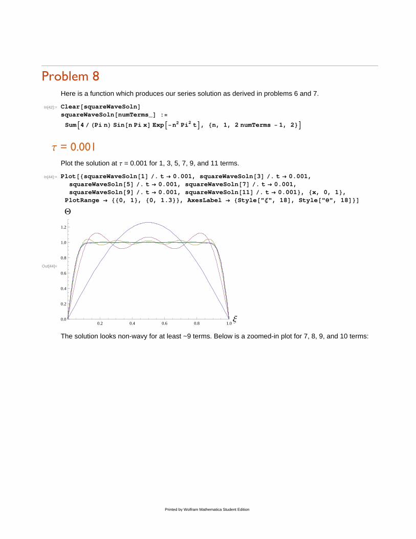
Problem 8 Here is a function which produces our series solution as derived in problems 6 and 7.

In[42]:= Clear@squareWaveSolnD squareWaveSoln@numTerms_D :=

SumA4 ê HPi nL Sin@n Pi xD ExpA-n2 Pi2 tE, 8n, 1, 2 numTerms - 1, 2<E

t = 0.001 Plot the solution at t = 0.001 for 1, 3, 5, 7, 9, and 11 terms.

In[44]:= Plot@8squareWaveSoln@1D ê. t Ø 0.001, squareWaveSoln@3D ê. t Ø 0.001, squareWaveSoln@5D ê. t Ø 0.001, squareWaveSoln@7D ê. t Ø 0.001, squareWaveSoln@9D ê. t Ø 0.001, squareWaveSoln@11D ê. t Ø 0.001<, 8x, 0, 1<,

PlotRange Ø 880, 1<, 80, 1.3<<, AxesLabel Ø 8Style@"x", 18D, Style@"Q", 18D<D

Q

Out[44]=

x0.0

0.2

0.4

0.6

0.8

1.0

1.2

0.2 0.4 0.6 0.8 1.0

The solution looks non-wavy for at least ~9 terms. Below is a zoomed-in plot for 7, 8, 9, and 10 terms:


mailto:squareWaveSoln@11D�.t





mailto:Plot@8squareWaveSoln@1D�.t

2

In[45]:= Plot@8squareWaveSoln@7D ê. t Ø 0.001, squareWaveSoln@8D ê. t Ø 0.001, squareWaveSoln@9D ê. t Ø 0.001, squareWaveSoln@10D ê. t Ø 0.001<, 8x, 0, 1<,

PlotRange Ø 880, 1<, 80.95, 1.05<<, AxesLabel Ø 8Style@"x", 18D, Style@"Q", 18D<D

Q

Out[45]=

0.2 0.4 0.6 0.8 1.0 x

0.96

0.98

1.00

1.02

1.04

8 terms has fewer than 10% deviation from the actual solution (i.e., it stays between 0.9 and 1.1 in the middle of the domain), so that would be an appropiate choice for sufficient terms to say it has con-verged. I’ll go with 10 terms because it looks like that gives less than 1% deviation, which is even better.

t = 0.1 Plot the solution at t = 0.001 for 1, 3, 5, 7, 9, and 11 terms.

In[46]:= Plot@8squareWaveSoln@1D ê. t Ø 0.1, squareWaveSoln@3D ê. t Ø 0.1, squareWaveSoln@5D ê. t Ø 0.1, squareWaveSoln@7D ê. t Ø 0.1, squareWaveSoln@9D ê. t Ø 0.1, squareWaveSoln@11D ê. t Ø 0.1<, 8x, 0, 1<,

PlotRange Ø 880, 1<, 80, 0.6<<, AxesLabel Ø 8Style@"x", 18D, Style@"Q", 18D<D

Out[46]=

x0.0

0.1

0.2

0.3

0.4

0.5

0.6

Q

0.2 0.4 0.6 0.8 1.0

Wow! All of the curves look the same. Even if you zoom way in, the solutions for 1, 2, and 3 terms look identical:












3

In[47]:= Plot@8squareWaveSoln@1D ê. t Ø 0.1, squareWaveSoln@2D ê. t Ø 0.1, squareWaveSoln@3D ê. t Ø 0.1<, 8x, 0, 1<,

PlotRange Ø 880, 1<, 80.3, 0.5<<, AxesLabel Ø 8Style@"x", 18D, Style@"Q", 18D<D

Q 0.50

0.45

Out[47]= 0.40

0.35

0.30 x0.2 0.4 0.6 0.8 1.0

At late times, only one term is needed to get a good approximation to the solution. That is because the solution contains e -n2 p t, so if t is anything but tiny, the exponential term kills the large-n terms. How-ever, at short times, you must include more terms because the exponential does not kill the higher order terms.

Problem 9 Plot the solution at various times:





4

In[48]:= Show@Plot@8squareWaveSoln@50D ê. t Ø 0.0001, squareWaveSoln@10D ê. t Ø 0.001, squareWaveSoln@5D ê. t Ø 0.01, squareWaveSoln@1D ê. t Ø 0.1, squareWaveSoln@1D ê. t Ø 0.5, squareWaveSoln@1D ê. t Ø 1<,

8x, 0, 1<, PlotRange Ø 880, 1<, 80, 1.2<<, PlotStyle Ø 8Red, Orange, Green, Blue, Purple, Black<, AxesLabel Ø 8Style@"x", 18D, Style@"Q", 18D<D,

Graphics@8Red, Text@Style@"t = 0.0001", 16D, 80.9, 1.1<D, Orange, Text@Style@"t = 0.001", 16D, 80.6, 1.1<D, Green, Text@Style@"t = 0.01", 16D, 80.5, 0.9<D, Blue, Text@Style@"t = 0.1", 16D, 80.5, 0.6<D, Purple, Text@Style@"t = 0.5", 16D,

80.5, 0.2<D, Black, Text@Style@"t = 1", 16D, 80.5, 0.08<D<DD

Out[48]=

t = 0.0001t = 0.001

t = 0.01

t = 0.1

t = 0.5 t = 1

x0.0

0.2

0.4

0.6

0.8

1.0

1.2

Q

0.2 0.4 0.6 0.8 1.0

The plot above demonstrates the complete thermal evolution of the heating/cooling of a 1D cartesian geometry with a fixed Q value at x = 0 and 1. Notice that by t = 1, the evolution is “finished.” Of course it will asymptotically approach a uniform temperature, but for engineering purposes, it has reached steady-state.

Cool aside: at early times, the heat hasn’t penetrated into the bulk yet, and only the edges of the domain have been affected. This is because at early times, the domain looks like a semi-infinite solid because the heat from one side hasn’t had a chance to start overlapping with the heat comming in through the other side. The solution for semi-infinite solids is and Erf, and indeed, the thermal profiles at the edges look just like erfs! The overlap is pretty much perfect (see below plot). That is because in the limit of small times, the series solution you derived here converges to the series expansion for erf. Cool...

In[49]:= Show@Plot@8squareWaveSoln@50D ê. t Ø 0.0001, squareWaveSoln@10D ê. t Ø 0.001, squareWaveSoln@5D ê. t Ø 0.01, squareWaveSoln@1D ê. t Ø 0.1, squareWaveSoln@1D ê. t Ø 0.5, squareWaveSoln@1D ê. t Ø 1<,

8x, 0, 1<, PlotRange Ø 880, 0.4<, 80, 1.2<<, PlotStyle Ø 8Red, Orange, Green, Blue, Purple, Black<, AxesLabel Ø 8Style@"x", 18D, Style@"Q", 18D<, PlotLabel Ø Style@"solid = series solutions, dashed = erf solutions", 20DD,

Plot@8Erf@x ê 0.02D, Erf@x ê 0.063D, Erf@x ê 0.2D<, 8x, 0, 0.4<, PlotStyle Ø 88Red, [email protected], [email protected], 0.05<D<,

8Orange, [email protected], [email protected], 0.05<D<,8Green, [email protected], [email protected], 0.05<D<<DD

Out[49]= $Aborted


mailto:[email protected]











mailto:Show@Plot@8squareWaveSoln@50D�.t






mailto:Show@Plot@8squareWaveSoln@50D�.t

5

2 real-world examples

This could be modelling the case of a long, wide sheet of material which is initially hot and is quenched in a fluid with a sufficiently high heat transfer coefficient that the Biot number is greater than 10. You could imagine casting a 10cm-thick sheet of steel that is ~900 C (just solidified) and quenching it in agitated brine at 25 C, for example.

Another example could be our graphite cube from problem 1 if it were in the 1D regime, i.e., only conduc-tion along the z-axis mattered, and basal plane conduction is very slow. This would model the tempera-ture profile vs. time as the cube was cooled from 298 K with a fixed surface temperature of 3 K.

A different set of boundary conditions

This solution is symmetric about x = 0.5. At that point, the temperature profile is always flat, i.e., !Q/!x = 0 at x = 0.5. This is consistent with the boundary condition of no heat flux at x = 0.5. This could be achieved, for example, by perfectly insulating the body on one side, at x = 0.5, and fixing the surface tempearture on the other side, at x = 0. The intial condition is uniform temperature within the body, which is different than the temperature at the x = 0 surface.

Q

x0.0

0.2

0.4

0.6

0.8

1.0

0.1 0.2 0.3 0.4 0.5

Thinking in terms of Biot number, this is like a high (>10) Biot number on the x = 0 side and a low (<0.1) Biot number on the x = 0.5 side. This could be achieved if you were cooling a sheet of freshly-cast steel by spraying it with brine on one side to fix the temperature, but the other side is in stagnant air, which practically does no cooling at all.


MIT OpenCourseWarehttp://ocw.mit.edu

3.044 Materials ProcessingSpring 2013

For information about citing these materials or our Terms of Use, visit: http://ocw.mit.edu/terms.

http://ocw.mit.edu/terms

http://ocw.mit.edu

Documents

10 C-AKkc, IN - MIT OpenCourseWare · Solve the conduction equation in radial coordinates, in 1D, with heat generation, and apply the boundary conditions