1 Visual Grouping by Neural Oscillator Networks - MITweb.mit.edu/nsl/www/preprints/visual_oscillators.pdf · Visual Grouping by Neural Oscillator Networks ... State-of-the-art visual

1

Visual Grouping by Neural Oscillator Networks

Guoshen Yu Jean-Jacques Slotine

Abstract

Distributed synchronization is known to occur at several scales in the brain, and has been suggested

as playing a key functional role in perceptual grouping. State-of-the-art visual grouping algorithms,

however, seem to give comparatively little attention to neural synchronization analogies. Based on the

framework of concurrent synchronization of dynamical systems, simple networks of neural oscillators

coupled with diffusive connections are proposed to solve visual grouping problems. The key idea is to

embed the desired grouping properties in the choice of the diffusive couplings, so that synchronization

of oscillators within each group indicates perceptual grouping of the underlying stimulative atoms,

while desynchronization between groups corresponds to group segregation. Compared with state-of-the-

art approaches, the same algorithm is shown to achieve promising results on several classical visual

grouping problems, including point clustering, contour integration, and image segmentation.

I. INTRODUCTION

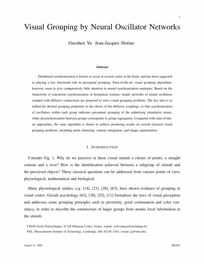
Consider Fig. 1. Why do we perceive in these visual stimuli a cluster of points, a straight

contour and a river? How is the identification achieved between a subgroup of stimuli and

the perceived objects? These classical questions can be addressed from various points of view,

physiological, mathematical and biological.

Many physiological studies, e.g. [14], [23], [28], [63], have shown evidence of grouping in

visual cortex. Gestalt psychology [62], [38], [25], [11] formalizes the laws of visual perception

and addresses some grouping principles such as proximity, good continuation and color con-

stancy, in order to describe the construction of larger groups from atomic local information in

the stimuli.

CMAP, Ecole Polytechnique, 91128 Palaiseau Cedex, France. (email: [email protected])

NSL, Massachusetts Institute of Technology, Cambridge, MA 02139, USA. (email: [email protected])

August 31, 2009 DRAFT

2

Fig. 1. Left: a cloud of points in which a dense cluster is embedded. Middle: a random direction grid in which a vertical

contour is embedded. Right: an image in which a river is embedded.

In computer vision, visual grouping has been studied in various mathematical frameworks

including graph-based methods [43], [20] and in particular normalized cuts [49], [8], harmonic

analysis [36], probabilistic approaches [12], [10], [9], [11], variational formulations [41], [40],

[1], Markov Random Fields [18], statistical techniques [16], [6], [7], [35], [34], among oth-

ers [53], [44].

In the brain, at a finer level of functional detail, the distributed synchronization known to

occur at different scales has been proposed as a general functional mechanism for perceptual

grouping [4], [50], [61]. In computer vision, however, comparatively little attention has been

devoted to exploiting neural-like oscillators in visual grouping. Wang and his colleagues have

performed very innovative work using oscillators for image segmentation [52], [57], [58], [33],

[5] and have extended the scheme to auditory segregation [2], [55], [56]. They constructed

oscillator networks with local excitatory lateral connections and a global inhibitory connection.

Adopting similar ideas, Yen and Finkel have simulated facilitatory and inhibitory interactions

among oscillators to conduct contour integration [63]. Li has proposed elaborate visual cortex

models with oscillators and applied them on lattice drawings segmentation [29], [30], [31],

[32]. Kuzmina and his colleagues [26], [27] have constructed a simple self-organized oscillator

coupling model, and applied it on synthetic lattice images as well. Faugeras et al. have started

studying oscillatory neural mass models in the contexts of natural and machine vision [13].

Inspired by neural synchronization mechanisms in perceptual grouping, this paper proposes a

simple and general neural oscillator algorithm for visual grouping, based on diffusive connections


3

and concurrent synchronization [45]. The key idea is to embed the desired grouping properties

in the choice of diffusive couplings between oscillators, so that the oscillators synchronize if

their underlying visual stimulative atoms belong to the same visual group and desynchronize

otherwise. A feedback mechanism and a multi-layer extension inspired by the hierarchical visual

cortex are introduced. The same algorithm is applied to point clustering, contour integration and

image segmentation.

The paper is organized as follows. Section II introduces a basic model of neural oscillators with

diffusive coupling connections, and proposes a general visual grouping algorithm. Sections III, IV

and V describe in detail the neural oscillator implementation for point clustering, contour inte-

gration and image segmentation and show a number of examples. The results are compared with

normalized cuts, a popular computer vision method [49], [8]. Section VI presents brief concluding

remarks. As detailed in Sec II-F, the method differs from the work of Wang et al [52], [57],

[58], [33], [5] in several fundamental aspects, including the synchronization/desynchronization

mechanism and the coupling structure.

II. MODEL AND ALGORITHM

The model is a network of neural oscillators coupled with diffusive connections. Each oscillator

is associated to an atomic element in the stimuli, for example a point, an orientation or a pixel.

Without coupling, the oscillators are desynchronized and oscillate in random phases. Under

diffusive coupling with the coupling strength appropriately tuned, they may converge to multiple

groups of synchronized elements. The synchronization of oscillators within each group indicates

the perceptual grouping of the underlying stimulative atoms, while the desynchronization between

groups suggests group segregation.

A. Neural Oscillators

A neural oscillator is an elementary unit associated to an atomic element in the stimuli, and

it models the perception of the stimulative atom. We use a modified form of FitzHugh-Nagumo


4

neural oscillators [15], [42], similar to [33], [5],

vi = 3vi − v3i − v7

i + 2− wi + Ii (1)

wi = c[α(1 + tanh(ρvi))− wi] (2)

where vi is the membrane potential of the oscillator, wi is an internal state variable representing

gate voltage, Ii represents the external current input and α, ρ and c are strictly positive constants.

This elementary unit oscillates if Ii exceeds a certain threshold and α, ρ and c are in an

appropriate range (within this range, the grouping results have low sensitivities to the values of

α, ρ and c — in all experiments we use α = 12, c = 0.04, ρ = 4). Fig. 2-a. plots the oscillation

trace of membrane potential vi. Other spiking oscillator models can be used similarly.

B. Diffusive Connections

Oscillators are coupled to form a network which aggregates the perception of individual atoms

in the visual stimulus. The oscillators are coupled through diffusive connections.

Let us denote by xi = [vi, wi]T the state vectors of the oscillators introduced in Section II-A,

each with dynamics xi = f(xi, t). A neural oscillator network is composed of N oscillators,

connected with diffusive coupling [59]

xi = f(xi, t) +∑

i6=j

kij(xj − xi), i = 1, . . . , N (3)

where kij is the coupling strength.

Oscillators i and j are said to be synchronized if xi remains equal to xj . Once the elements

are synchronized, the coupling terms in (3) disappear, so that each individual element exhibits

its natural and uncoupled behavior, as illustrated in Fig. 2. A larger value of kij tends to reduce

the state difference xi − xj and thus to reinforce the synchronization between oscillators i and

j (see the Appendix for more details).

The key to using diffusively-coupled neural oscillators for visual grouping is to tune the

couplings so that the oscillators synchronize if their underlying atoms belong to the same visual

group, and desynchronize otherwise. According to Gestalt psychology [62], [25], [38], visual

stimulative atoms having similarity (e.g. gray-level, color, orientation) or proximity tend to be


5

a b

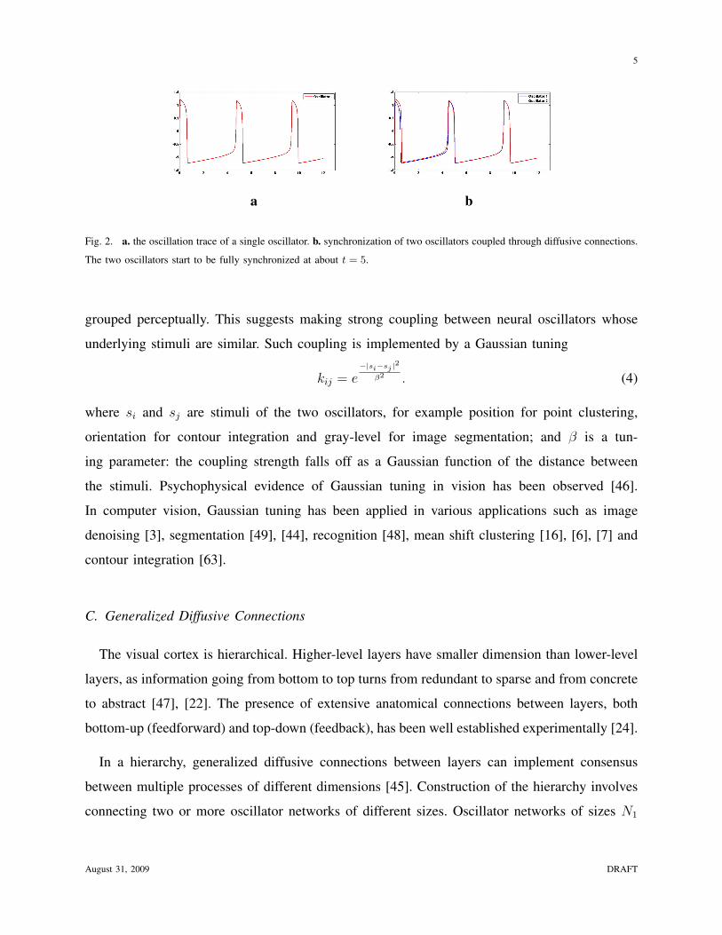
Fig. 2. a. the oscillation trace of a single oscillator. b. synchronization of two oscillators coupled through diffusive connections.

The two oscillators start to be fully synchronized at about t = 5.

grouped perceptually. This suggests making strong coupling between neural oscillators whose

underlying stimuli are similar. Such coupling is implemented by a Gaussian tuning

kij = e−|si−sj |2

β2 . (4)

where si and sj are stimuli of the two oscillators, for example position for point clustering,

orientation for contour integration and gray-level for image segmentation; and β is a tun-

ing parameter: the coupling strength falls off as a Gaussian function of the distance between

the stimuli. Psychophysical evidence of Gaussian tuning in vision has been observed [46].

In computer vision, Gaussian tuning has been applied in various applications such as image

denoising [3], segmentation [49], [44], recognition [48], mean shift clustering [16], [6], [7] and

contour integration [63].

C. Generalized Diffusive Connections

The visual cortex is hierarchical. Higher-level layers have smaller dimension than lower-level

layers, as information going from bottom to top turns from redundant to sparse and from concrete

to abstract [47], [22]. The presence of extensive anatomical connections between layers, both

bottom-up (feedforward) and top-down (feedback), has been well established experimentally [24].

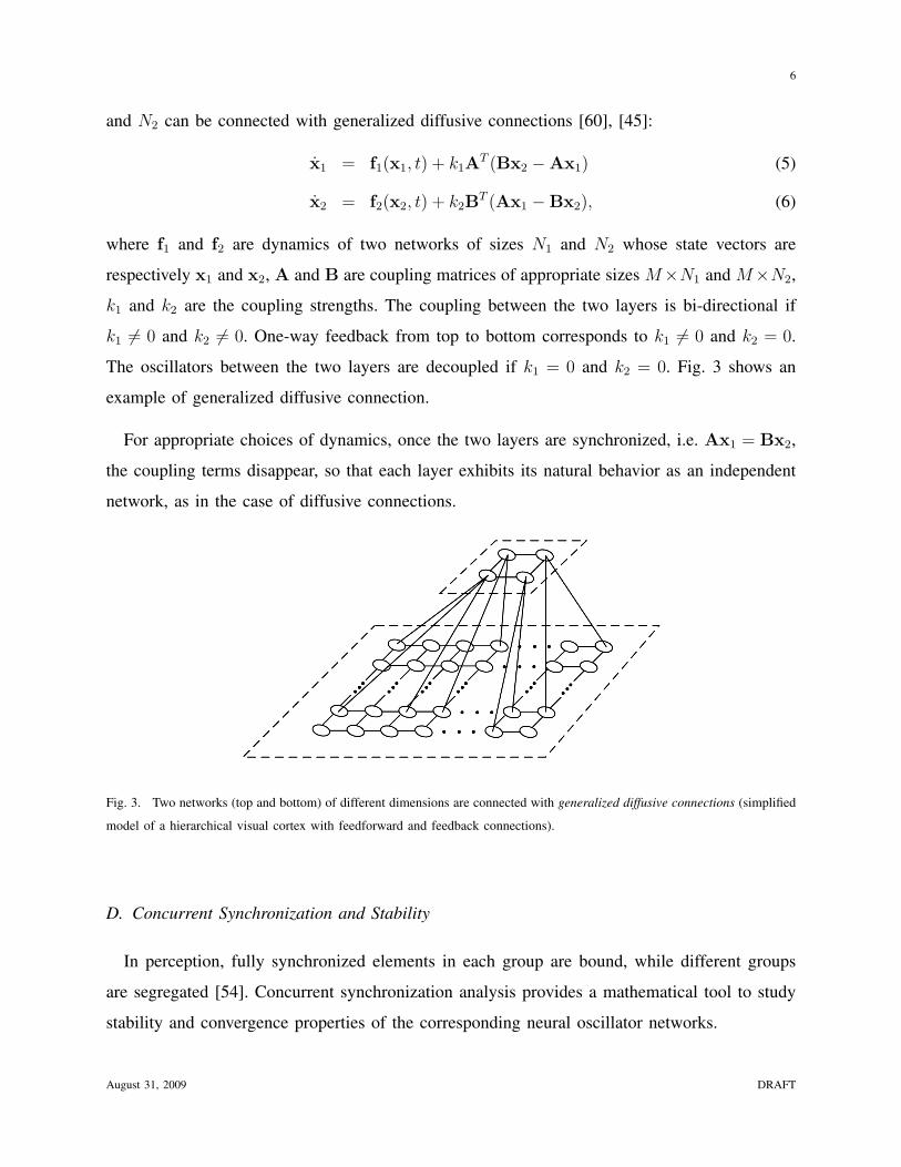
In a hierarchy, generalized diffusive connections between layers can implement consensus

between multiple processes of different dimensions [45]. Construction of the hierarchy involves

connecting two or more oscillator networks of different sizes. Oscillator networks of sizes N1


6

and N2 can be connected with generalized diffusive connections [60], [45]:

x1 = f1(x1, t) + k1AT (Bx2 −Ax1) (5)

x2 = f2(x2, t) + k2BT (Ax1 −Bx2), (6)

where f1 and f2 are dynamics of two networks of sizes N1 and N2 whose state vectors are

respectively x1 and x2, A and B are coupling matrices of appropriate sizes M×N1 and M×N2,

k1 and k2 are the coupling strengths. The coupling between the two layers is bi-directional if

k1 6= 0 and k2 6= 0. One-way feedback from top to bottom corresponds to k1 6= 0 and k2 = 0.

The oscillators between the two layers are decoupled if k1 = 0 and k2 = 0. Fig. 3 shows an

example of generalized diffusive connection.

For appropriate choices of dynamics, once the two layers are synchronized, i.e. Ax1 = Bx2,

the coupling terms disappear, so that each layer exhibits its natural behavior as an independent

network, as in the case of diffusive connections.

Fig. 3. Two networks (top and bottom) of different dimensions are connected with generalized diffusive connections (simplified

model of a hierarchical visual cortex with feedforward and feedback connections).

D. Concurrent Synchronization and Stability

In perception, fully synchronized elements in each group are bound, while different groups

are segregated [54]. Concurrent synchronization analysis provides a mathematical tool to study

stability and convergence properties of the corresponding neural oscillator networks.


7

In an ensemble of dynamical elements, concurrent synchronization is defined as a regime

where the whole system is divided into multiple groups of fully synchronized elements, but

elements from different groups are not necessarily synchronized [45]. Networks of oscillators

coupled by diffusive connections or generalized diffusive connections defined in Sections II-B

and II-C are specific cases of this general framework [45], [59].

A subset of the global state space is called invariant if trajectories that start in that subset

remain in that subset. In our synchronization context, the invariant subsets of interest are linear

subspaces, corresponding to some components of the overall state being equal (xi = xj) in (3),

or verifying some linear relation (Ax1 = Bx2) in (5, 6). Concurrent synchronization analysis

quantifies stability and convergence to invariant linear subspaces. Furthermore, a property of

concurrent synchronization analysis, which turns out to be particularly convenient in the context

of grouping, is that the actual invariant subset itself needs not be known a priori to guarantee

stable convergence to it.

Concurrent synchronization may first be studied in an idealized setting, e.g., with exactly equal

inputs to groups of oscillators, and noise-free conditions. This allows one to compute minimum

coupling gains to guarantee global exponential convergence to the invariant synchronization

subspace. Robustness of concurrent synchronization, a consequence of its exponential converge

properties, allows the qualitative behavior of the nominal model to be preserved even in non-

ideal conditions. In particular, it can be shown and quantified that for high convergence rates,

actual trajectories differ little from trajectories based on an idealized model [59].

A more specific discussion of stability and convergence is given in the appendix. The reader

is referred to [45] for more details on the analysis tools.

E. Visual Grouping Algorithm

A basic and general visual grouping algorithm is obtained by constructing a neural oscillator

network according to the following steps.

1) Construct a neural oscillator network. Each oscillator (1, 2) is associated to one atom in the

stimuli. Oscillators are connected with diffusive connections (3) or generalized diffusive


8

connections (5, 6) using the Gaussian-tuned gains (4). The coupling tuning for point

clustering, contour integration and image segmentation will be specified in the following

Sections.

2) Simulate the so-constructed network. The oscillators converge to concurrently synchronized

groups.

3) Identify the synchronized oscillators and equivalently the visual groups. A group of syn-

chronized oscillators indicates that the underlying visual stimulative atoms are perceptually

grouped. Desynchronization between groups suggests that the underlying stimulative atoms

in the two groups are segregated.

The differential equations (1) and (2) are solved using a Runge-Kutta method (with the Matlab

ODE solver). As a consequence of the global exponential convergence of networks of oscillators

coupled by diffusive coupling [59], concurrent synchronization in the neural oscillator networks

typically can occur within 2 or 3 cycles, and it may be verified by checking the correlation among

the traces in potential groups [63]. Fast transients are also consistent with the biological analogy,

as in the brain concurrent synchronization is thought to occur transiently over a few oscillation

cycles [4]. Once the system converges to the invariant synchronization subspace, synchronization

can be identified. As shown in Figs. 4-b and 5-b, traces of synchronized oscillators coincide in

time, while those of desynchronized groups are separated [54]. For point clustering and contour

integration, the identification of synchronization in the oscillation traces is implemented by

thresholding the correlation among the traces as proposed in [63]. For image segmentation,

a k-means algorithm (with random initialization and correlation distance measure) is applied

on the oscillation traces to identify the synchronization. A complete description of the basic

image segmentation algorithm is given in Fig. 10, which applies to point clustering and contour

integration as well. Feedback and multi-layer network extensions for image segmentation are

detailed in Figs. 14 and 18.

As in most other visual grouping algorithms [49], [7], [44], [63], some parameters, including

the number of clusters and a Gaussian tuning parameter, need to be adjusted manually according

to the number and size of the groups that one expects to obtain. Automatic parameter selection

in visual grouping problems remains an active research topic in computer vision [51] and is out

of the scope of the present paper which emphasizes neural analogy and implementation.


9

F. Relation to Previous Work

Among the relatively small body of previous work based on neural oscillators mentioned

in Section I, the pioneering work of Wang et al. [52], [57], [58], [5] on image segmentation

called LEGION (locally excitatory globally inhibitory oscillator networks) is most related to the

present paper. Yen and Finkel [63] have studied similar ideas for contour integration. While its

starting point is the same, namely achieving grouping through oscillator synchronization and

tight coupling between oscillators associated to similar stimuli, the method presented in this

paper differs fundamentally from LEGION in the following aspects:

• Synchronization mechanism. A global inhibitor that allows active oscillators to inhibit

others is a key element in LEGION in order to achieve synchronization within one group

and distinction between different groups: at one time only one group of oscillators is active

and the others are inhibited. The present work relies on concurrent synchronization [45] and

does not contain any inhibitor: all oscillators are active simultaneously; multiple groups of

oscillators, synchronized within each group and desynchronized between groups, coexist.

• Coupling mechanism. The oscillators coupling in LEGION is obtained through stimulation:

local excitation coupling is implemented through positive stimulation which tends to activate

the oscillators in the neighborhood; global inhibition is obtained by negative stimulation

which tends to deactivate other oscillators. The coupling in the present work is based on

diffusive connections (3): the coupling term is a state difference which tends to zero as

synchronization occurs [59].

• Robustness. The original LEGION was shown to be sensitive to noise [52], [57]. A concept

of lateral potential for each oscillator was introduced in a later version of LEGION [58],

[5] to improve its robustness and reduce over-segmentation in real image applications. The

proposed method based on non-local diffusive connections has inherent robustness to noise.

In turn, these fundamental differences make the proposed neural oscillator framework fairly

simple and general. It provides solutions not only for image segmentation, but also for point

clustering and contour integration, as detailed in the following Sections.


10

III. POINT CLUSTERING

Point clustering with neural oscillators is based on diffusive connections (3) and follows

directly the general algorithm in Section II-E. Let us denote ci = (ix, iy) the coordinates of a

point pi. Each point pi is associated to an oscillator xi. The proximity Gestalt principle [62],

[25], [38] suggests strong coupling between oscillators corresponding to proximate points. More

precisely, the coupling strength between xi and xj is

kij =

e−|ci−cj |2

β2 if j ∈ Ni

0 otherwise, (7)

where Ni is the set of M points closest to pi: an oscillator xi is coupled with its M nearest

neighbors. Oscillators may be indirectly coupled over larger distances through synchronization

propagation (e.g., if x1 is coupled with x2 and x2 is coupled with x3, then x1 is indirectly

coupled with x3.) β is the main parameter which tunes the coupling. It is adjusted according to

the size of the clusters one expects to detect, with a larger β tending to result in bigger clusters.

M is a more minor regularization parameter, and the clustering has low sensitivity to M once it

is larger than 5. In the experiments, the parameters are configured as β = 3 and M = 10. The

external inputs Ii of the oscillators in (1) are chosen as uniformly distributed random variables

in the appropriate range.

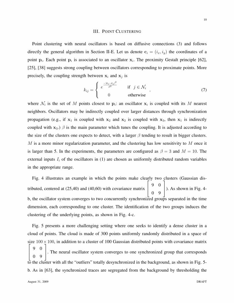
Fig. 4 illustrates an example in which the points make clearly two clusters (Gaussian dis-

tributed, centered at (25,40) and (40,60) with covariance matrix

9 0

0 9

). As shown in Fig. 4-

b, the oscillator system converges to two concurrently synchronized groups separated in the time

dimension, each corresponding to one cluster. The identification of the two groups induces the

clustering of the underlying points, as shown in Fig. 4-c.

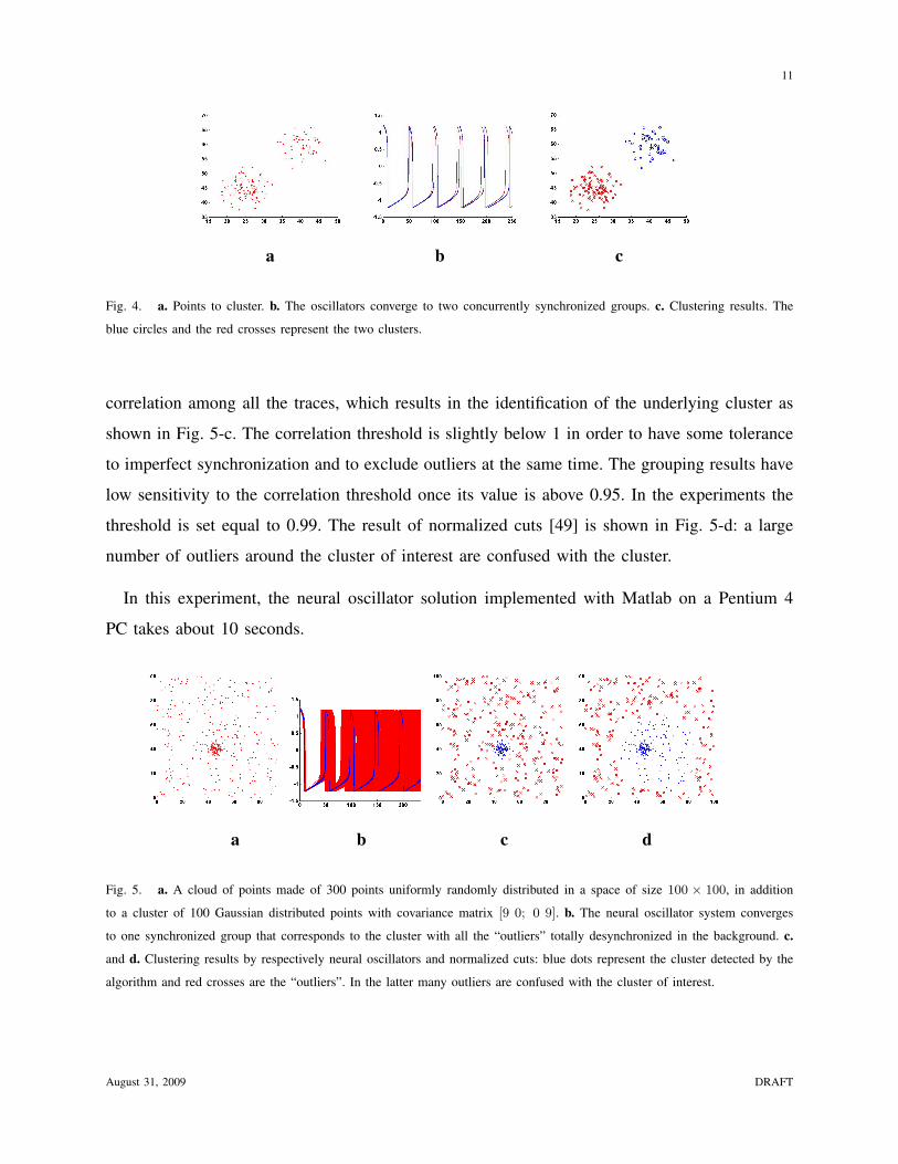
Fig. 5 presents a more challenging setting where one seeks to identify a dense cluster in a

cloud of points. The cloud is made of 300 points uniformly randomly distributed in a space of

size 100×100, in addition to a cluster of 100 Gaussian distributed points with covariance matrix 9 0

0 9

. The neural oscillator system converges to one synchronized group that corresponds

to the cluster with all the “outliers” totally desynchronized in the background, as shown in Fig. 5-

b. As in [63], the synchronized traces are segregated from the background by thresholding the


11

a b c

Fig. 4. a. Points to cluster. b. The oscillators converge to two concurrently synchronized groups. c. Clustering results. The

blue circles and the red crosses represent the two clusters.

correlation among all the traces, which results in the identification of the underlying cluster as

shown in Fig. 5-c. The correlation threshold is slightly below 1 in order to have some tolerance

to imperfect synchronization and to exclude outliers at the same time. The grouping results have

low sensitivity to the correlation threshold once its value is above 0.95. In the experiments the

threshold is set equal to 0.99. The result of normalized cuts [49] is shown in Fig. 5-d: a large

number of outliers around the cluster of interest are confused with the cluster.

In this experiment, the neural oscillator solution implemented with Matlab on a Pentium 4

PC takes about 10 seconds.

a b c d

Fig. 5. a. A cloud of points made of 300 points uniformly randomly distributed in a space of size 100 × 100, in addition

to a cluster of 100 Gaussian distributed points with covariance matrix [9 0; 0 9]. b. The neural oscillator system converges

to one synchronized group that corresponds to the cluster with all the “outliers” totally desynchronized in the background. c.

and d. Clustering results by respectively neural oscillators and normalized cuts: blue dots represent the cluster detected by the

algorithm and red crosses are the “outliers”. In the latter many outliers are confused with the cluster of interest.


12

IV. CONTOUR INTEGRATION

Field et al. [14] have performed interesting experiments to test human capacity of contour

integration, i.e., of identifying a path within a field of randomly-oriented Gabor elements. They

made some quantitative observations in accordance with the Gestalt “good continuation” law [62],

[63]:

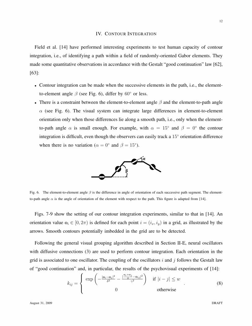
• Contour integration can be made when the successive elements in the path, i.e., the element-

to-element angle β (see Fig. 6), differ by 60◦ or less.

• There is a constraint between the element-to-element angle β and the element-to-path angle

α (see Fig. 6). The visual system can integrate large differences in element-to-element

orientation only when those differences lie along a smooth path, i.e., only when the element-

to-path angle α is small enough. For example, with α = 15◦ and β = 0◦ the contour

integration is difficult, even though the observers can easily track a 15◦ orientation difference

when there is no variation (α = 0◦ and β = 15◦).

Fig. 6. The element-to-element angle β is the difference in angle of orientation of each successive path segment. The element-

to-path angle α is the angle of orientation of the element with respect to the path. This figure is adapted from [14].

Figs. 7-9 show the setting of our contour integration experiments, similar to that in [14]. An

orientation value oi ∈ [0, 2π) is defined for each point i = (ix, iy) in a grid, as illustrated by the

arrows. Smooth contours potentially imbedded in the grid are to be detected.

Following the general visual grouping algorithm described in Section II-E, neural oscillators

with diffusive connections (3) are used to perform contour integration. Each orientation in the

grid is associated to one oscillator. The coupling of the oscillators i and j follows the Gestalt law

of “good continuation” and, in particular, the results of the psychovisual experiments of [14]:

kij =

exp

(− |oi−oj |2

δ2 − |oi+oj2

−oij |2γ2

)if |i− j| ≤ w

0 otherwise. (8)


13

where

oij =

θij if |θij − |oi+oj |2

| < |θij + π − |oi+oj |2

|θij + π otherwise

is the undirectional orientation of the path ij (the closest to the average element-to-element

orientation |oi+oj|2

modulo π), with θij = arctan( iy−jy

ix−jx). Oscillators with small element-to-element

angle β (the first term in (8)) and small element-to-path angle α (the second term in (8)) are

coupled more tightly. The neural oscillator system makes therefore smooth contour integration.

δ and γ tune the smoothness of the detected contour. As contour integration is known to be

rather local [14], the coupling (8) is effective within a neighborhood of size (2w+1)× (2w+1).

In the experiments the parameters are configured as δ = 20◦, γ = 10◦ and w = 1, in line with

the results of the psychovisual experiments of Field et al [14]. The external inputs Ii of the

oscillators in (1) are set proportional to the underlying orientations oi.

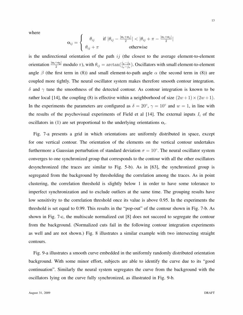
Fig. 7-a presents a grid in which orientations are uniformly distributed in space, except

for one vertical contour. The orientation of the elements on the vertical contour undertakes

furthermore a Gaussian perturbation of standard deviation σ = 10◦. The neural oscillator system

converges to one synchronized group that corresponds to the contour with all the other oscillators

desynchronized (the traces are similar to Fig. 5-b). As in [63], the synchronized group is

segregated from the background by thresholding the correlation among the traces. As in point

clustering, the correlation threshold is slightly below 1 in order to have some tolerance to

imperfect synchronization and to exclude outliers at the same time. The grouping results have

low sensitivity to the correlation threshold once its value is above 0.95. In the experiments the

threshold is set equal to 0.99. This results in the “pop-out” of the contour shown in Fig. 7-b. As

shown in Fig. 7-c, the multiscale normalized cut [8] does not succeed to segregate the contour

from the background. (Normalized cuts fail in the following contour integration experiments

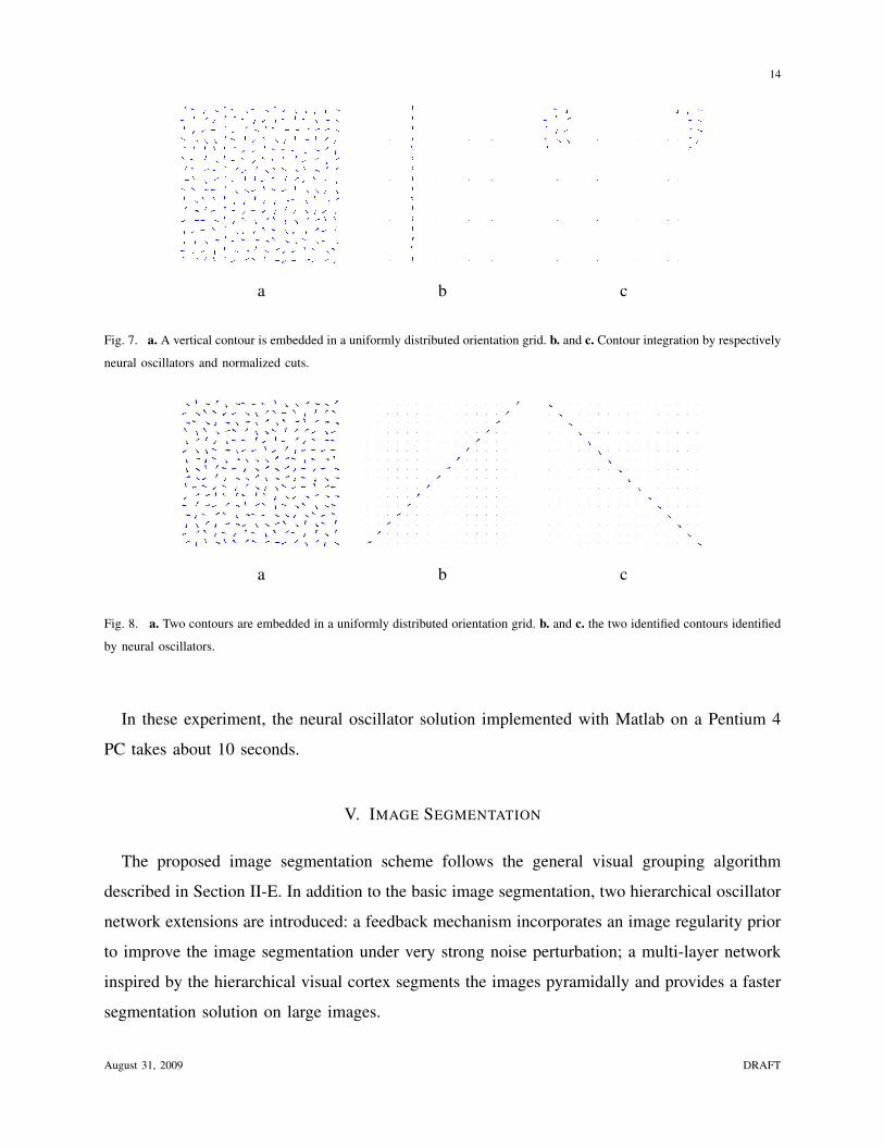
as well and are not shown.) Fig. 8 illustrates a similar example with two intersecting straight

contours.

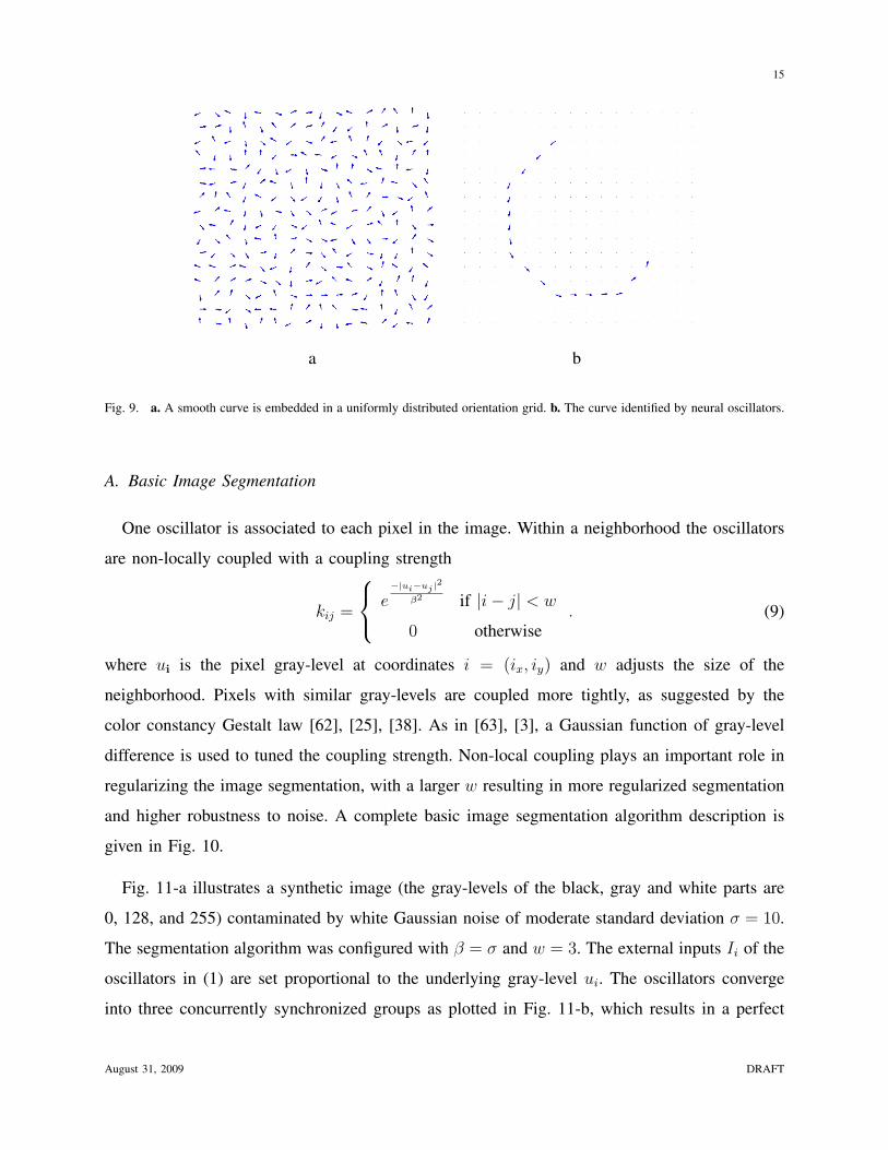
Fig. 9-a illustrates a smooth curve embedded in the uniformly randomly distributed orientation

background. With some minor effort, subjects are able to identify the curve due to its “good

continuation”. Similarly the neural system segregates the curve from the background with the

oscillators lying on the curve fully synchronized, as illustrated in Fig. 9-b.


14

a b c

Fig. 7. a. A vertical contour is embedded in a uniformly distributed orientation grid. b. and c. Contour integration by respectively

neural oscillators and normalized cuts.

a b c

Fig. 8. a. Two contours are embedded in a uniformly distributed orientation grid. b. and c. the two identified contours identified

by neural oscillators.

In these experiment, the neural oscillator solution implemented with Matlab on a Pentium 4

PC takes about 10 seconds.

V. IMAGE SEGMENTATION

The proposed image segmentation scheme follows the general visual grouping algorithm

described in Section II-E. In addition to the basic image segmentation, two hierarchical oscillator

network extensions are introduced: a feedback mechanism incorporates an image regularity prior

to improve the image segmentation under very strong noise perturbation; a multi-layer network

inspired by the hierarchical visual cortex segments the images pyramidally and provides a faster

segmentation solution on large images.


15

a b

Fig. 9. a. A smooth curve is embedded in a uniformly distributed orientation grid. b. The curve identified by neural oscillators.

A. Basic Image Segmentation

One oscillator is associated to each pixel in the image. Within a neighborhood the oscillators

are non-locally coupled with a coupling strength

kij =

e−|ui−uj |2

β2 if |i− j| < w

0 otherwise. (9)

where ui is the pixel gray-level at coordinates i = (ix, iy) and w adjusts the size of the

neighborhood. Pixels with similar gray-levels are coupled more tightly, as suggested by the

color constancy Gestalt law [62], [25], [38]. As in [63], [3], a Gaussian function of gray-level

difference is used to tuned the coupling strength. Non-local coupling plays an important role in

regularizing the image segmentation, with a larger w resulting in more regularized segmentation

and higher robustness to noise. A complete basic image segmentation algorithm description is

given in Fig. 10.

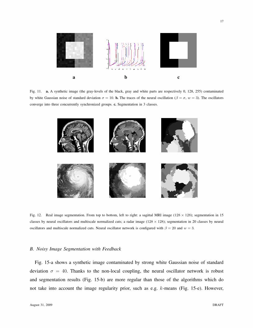
Fig. 11-a illustrates a synthetic image (the gray-levels of the black, gray and white parts are

0, 128, and 255) contaminated by white Gaussian noise of moderate standard deviation σ = 10.

The segmentation algorithm was configured with β = σ and w = 3. The external inputs Ii of the

oscillators in (1) are set proportional to the underlying gray-level ui. The oscillators converge

into three concurrently synchronized groups as plotted in Fig. 11-b, which results in a perfect


16

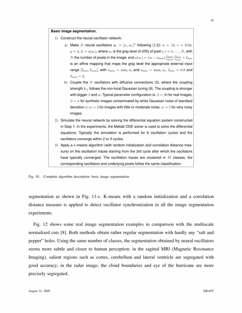
Basic image segmentation.

1) Construct the neural oscillator network.

a) Make N neural oscillators xi = [vi, wi]T following (1,2): α = 12, c = 0.04,

ρ = 4, Ii = a(ui), where ui is the gray level (0-255) of pixel i, i = 1, . . . , N , with

N the number of pixels in the image, and a(ui) = (ui−umin) Imax−Iminumax−umin

+ Imin

is an affine mapping that maps the gray level the appropriate external input

range [Imin, Imax], with umin = mini ui and umin = maxi ui, Imin = 0.8 and

Imax = 2.

b) Couple the N oscillators with diffusive connections (3), where the coupling

strength kij follows the non-local Gaussian tuning (9). The coupling is stronger

with bigger β and w. Typical parameter configuration is: β = 20 for real images,

β = σ for synthetic images contaminated by white Gaussian noise of standard

deviation σ; w = 3 for images with little or moderate noise, w = 5 for very noisy

images.

2) Simulate the neural network by solving the differential equation system constructed

in Step 1. In the experiments, the Matlab ODE solver is used to solve the differential

equations. Typically the simulation is performed for 6 oscillation cycles and the

oscillators converge within 2 or 3 cycles.

3) Apply a k-means algorithm (with random initialization and correlation distance mea-

sure) on the oscillation traces starting from the 3rd cycle after which the oscillators

have typically converged. The oscillation traces are clustered in M classes, the

corresponding oscillators and underlying pixels follow the same classification.

Fig. 10. Complete algorithm description: basic image segmentation.

segmentation as shown in Fig. 11-c. K-means with a random initialization and a correlation

distance measure is applied to detect oscillator synchronization in all the image segmentation

experiments.

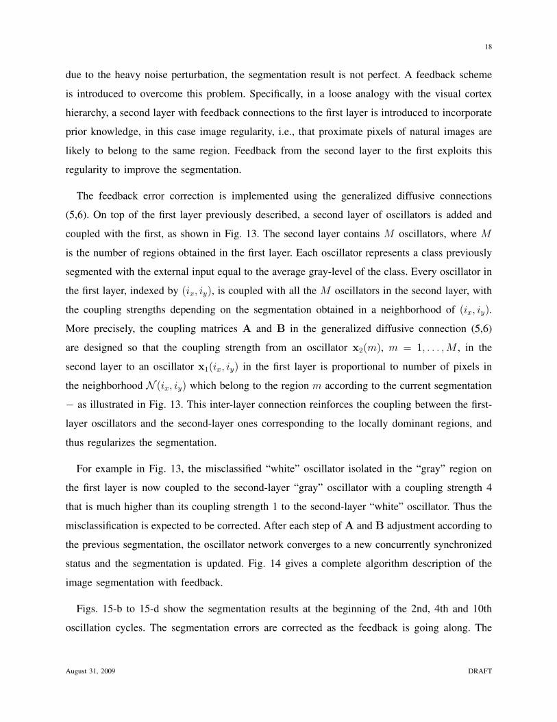
Fig. 12 shows some real image segmentation examples in comparison with the multiscale

normalized cuts [8]. Both methods obtain rather regular segmentation with hardly any “salt and

pepper” holes. Using the same number of classes, the segmentation obtained by neural oscillators

seems more subtle and closer to human perception: in the sagittal MRI (Magnetic Resonance

Imaging), salient regions such as cortex, cerebellum and lateral ventricle are segregated with

good accuracy; in the radar image, the cloud boundaries and eye of the hurricane are more

precisely segregated.


17

a b c

Fig. 11. a. A synthetic image (the gray-levels of the black, gray and white parts are respectively 0, 128, 255) contaminated

by white Gaussian noise of standard deviation σ = 10. b. The traces of the neural oscillation (β = σ, w = 3). The oscillators

converge into three concurrently synchronized groups. c. Segmentation in 3 classes.

Fig. 12. Real image segmentation. From top to bottom, left to right: a sagittal MRI image (128 × 128); segmentation in 15

classes by neural oscillators and multiscale normalized cuts; a radar image (128 × 128); segmentation in 20 classes by neural

oscillators and multiscale normalized cuts. Neural oscillator network is configured with β = 20 and w = 3.

B. Noisy Image Segmentation with Feedback

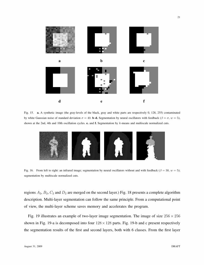
Fig. 15-a shows a synthetic image contaminated by strong white Gaussian noise of standard

deviation σ = 40. Thanks to the non-local coupling, the neural oscillator network is robust

and segmentation results (Fig. 15-b) are more regular than those of the algorithms which do

not take into account the image regularity prior, such as e.g. k-means (Fig. 15-e). However,


18

due to the heavy noise perturbation, the segmentation result is not perfect. A feedback scheme

is introduced to overcome this problem. Specifically, in a loose analogy with the visual cortex

hierarchy, a second layer with feedback connections to the first layer is introduced to incorporate

prior knowledge, in this case image regularity, i.e., that proximate pixels of natural images are

likely to belong to the same region. Feedback from the second layer to the first exploits this

regularity to improve the segmentation.

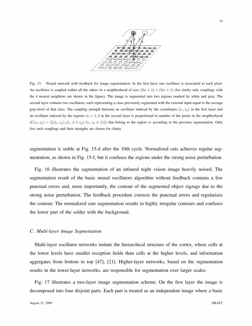
The feedback error correction is implemented using the generalized diffusive connections

(5,6). On top of the first layer previously described, a second layer of oscillators is added and

coupled with the first, as shown in Fig. 13. The second layer contains M oscillators, where M

is the number of regions obtained in the first layer. Each oscillator represents a class previously

segmented with the external input equal to the average gray-level of the class. Every oscillator in

the first layer, indexed by (ix, iy), is coupled with all the M oscillators in the second layer, with

the coupling strengths depending on the segmentation obtained in a neighborhood of (ix, iy).

More precisely, the coupling matrices A and B in the generalized diffusive connection (5,6)

are designed so that the coupling strength from an oscillator x2(m), m = 1, . . . , M , in the

second layer to an oscillator x1(ix, iy) in the first layer is proportional to number of pixels in

the neighborhood N (ix, iy) which belong to the region m according to the current segmentation

− as illustrated in Fig. 13. This inter-layer connection reinforces the coupling between the first-

layer oscillators and the second-layer ones corresponding to the locally dominant regions, and

thus regularizes the segmentation.

For example in Fig. 13, the misclassified “white” oscillator isolated in the “gray” region on

the first layer is now coupled to the second-layer “gray” oscillator with a coupling strength 4

that is much higher than its coupling strength 1 to the second-layer “white” oscillator. Thus the

misclassification is expected to be corrected. After each step of A and B adjustment according to

the previous segmentation, the oscillator network converges to a new concurrently synchronized

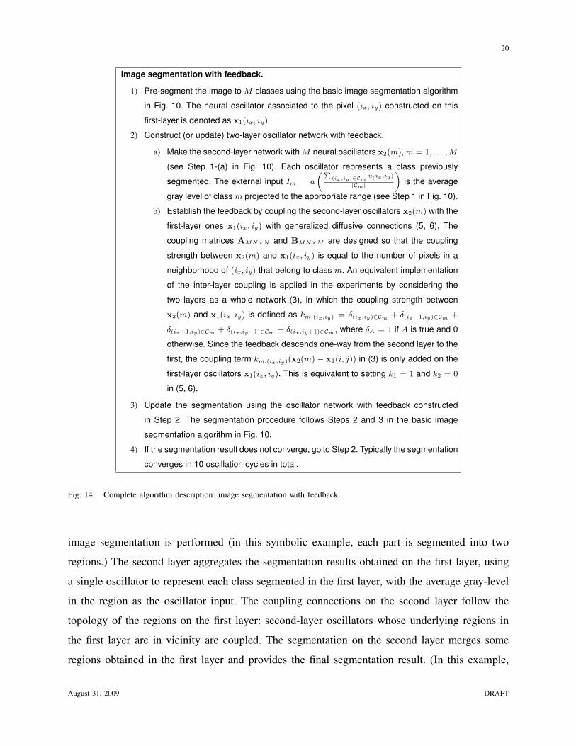
status and the segmentation is updated. Fig. 14 gives a complete algorithm description of the

image segmentation with feedback.

Figs. 15-b to 15-d show the segmentation results at the beginning of the 2nd, 4th and 10th

oscillation cycles. The segmentation errors are corrected as the feedback is going along. The


19

Fig. 13. Neural network with feedback for image segmentation. In the first layer one oscillator is associated to each pixel.

An oscillator is coupled within all the others in a neighborhood of size (2w + 1)× (2w + 1) (for clarity only couplings with

the 4 nearest neighbors are shown in the figure). The image is segmented into two regions marked by white and gray. The

second layer contains two oscillators, each representing a class previously segmented with the external input equal to the average

gray-level of that class. The coupling strength between an oscillator indexed by the coordinates (ix, iy) in the first layer and

an oscillator indexed by the regions m = 1, 2 in the second layer is proportional to number of the pixels in the neighborhood

N (ix, iy) = {((ix, iy), (ix ± 1, iy), (ix, iy ± 1))} that belong to the region m according to the previous segmentation. Only

five such couplings and their strengths are shown for clarity .

segmentation is stable at Fig. 15-d after the 10th cycle. Normalized cuts achieves regular seg-

mentation, as shown in Fig. 15-f, but it confuses the regions under the strong noise perturbation.

Fig. 16 illustrates the segmentation of an infrared night vision image heavily noised. The

segmentation result of the basic neural oscillators algorithm without feedback contains a few

punctual errors and, more importantly, the contour of the segmented object zigzags due to the

strong noise perturbation. The feedback procedure corrects the punctual errors and regularizes

the contour. The normalized cuts segmentation results in highly irregular contours and confuses

the lower part of the solder with the background.

C. Multi-layer Image Segmentation

Multi-layer oscillator networks imitate the hierarchical structure of the cortex, where cells at

the lower levels have smaller reception fields than cells at the higher levels, and information

aggregates from bottom to top [47], [21]. Higher-layer networks, based on the segmentation

results in the lower-layer networks, are responsible for segmentation over larger scales.

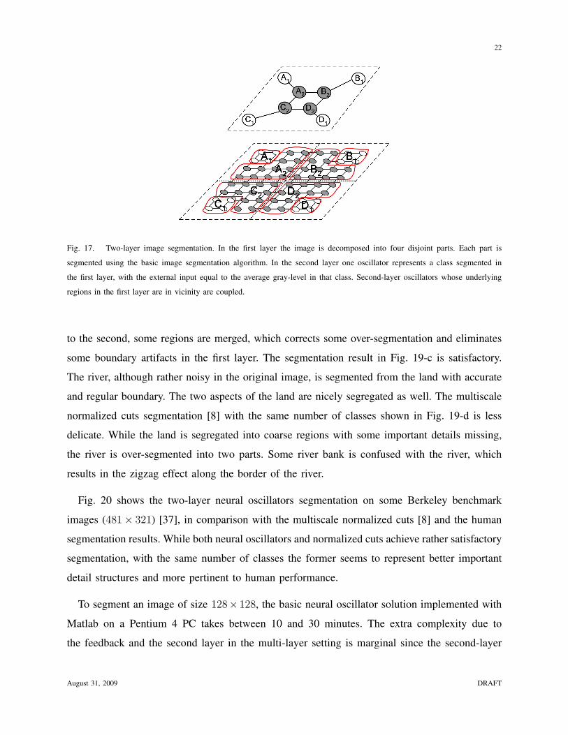
Fig. 17 illustrates a two-layer image segmentation scheme. On the first layer the image is

decomposed into four disjoint parts. Each part is treated as an independent image where a basic


20

Image segmentation with feedback.

1) Pre-segment the image to M classes using the basic image segmentation algorithm

in Fig. 10. The neural oscillator associated to the pixel (ix, iy) constructed on this

first-layer is denoted as x1(ix, iy).

2) Construct (or update) two-layer oscillator network with feedback.

a) Make the second-layer network with M neural oscillators x2(m), m = 1, . . . , M

(see Step 1-(a) in Fig. 10). Each oscillator represents a class previously

segmented. The external input Im = a

(∑(ix,iy)∈Cm

u(ix,iy)

|Cm|

)is the average

gray level of class m projected to the appropriate range (see Step 1 in Fig. 10).

b) Establish the feedback by coupling the second-layer oscillators x2(m) with the

first-layer ones x1(ix, iy) with generalized diffusive connections (5, 6). The

coupling matrices AMN×N and BMN×M are designed so that the coupling

strength between x2(m) and x1(ix, iy) is equal to the number of pixels in a

neighborhood of (ix, iy) that belong to class m. An equivalent implementation

of the inter-layer coupling is applied in the experiments by considering the

two layers as a whole network (3), in which the coupling strength between

x2(m) and x1(ix, iy) is defined as km,(ix,iy) = δ(ix,iy)∈Cm + δ(ix−1,iy)∈Cm +

δ(ix+1,iy)∈Cm + δ(ix,iy−1)∈Cm + δ(ix,iy+1)∈Cm , where δA = 1 if A is true and 0

otherwise. Since the feedback descends one-way from the second layer to the

first, the coupling term km,(ix,iy)(x2(m) − x1(i, j)) in (3) is only added on the

first-layer oscillators x1(ix, iy). This is equivalent to setting k1 = 1 and k2 = 0

in (5, 6).

3) Update the segmentation using the oscillator network with feedback constructed

in Step 2. The segmentation procedure follows Steps 2 and 3 in the basic image

segmentation algorithm in Fig. 10.

4) If the segmentation result does not converge, go to Step 2. Typically the segmentation

converges in 10 oscillation cycles in total.

Fig. 14. Complete algorithm description: image segmentation with feedback.

image segmentation is performed (in this symbolic example, each part is segmented into two

regions.) The second layer aggregates the segmentation results obtained on the first layer, using

a single oscillator to represent each class segmented in the first layer, with the average gray-level

in the region as the oscillator input. The coupling connections on the second layer follow the

topology of the regions on the first layer: second-layer oscillators whose underlying regions in

the first layer are in vicinity are coupled. The segmentation on the second layer merges some

regions obtained in the first layer and provides the final segmentation result. (In this example,


21

a b c

d e f

Fig. 15. a. A synthetic image (the gray-levels of the black, gray and white parts are respectively 0, 128, 255) contaminated

by white Gaussian noise of standard deviation σ = 40. b–d. Segmentation by neural oscillators with feedback (β = σ, w = 5),

shown at the 2nd, 4th and 10th oscillation cycles. e. and f. Segmentation by k-means and multiscale normalized cuts.

Fig. 16. From left to right: an infrared image; segmentation by neural oscillators without and with feedback (β = 30, w = 5);

segmentation by multiscale normalized cuts.

regions A2, B2, C2 and D2 are merged on the second layer.) Fig. 18 presents a complete algorithm

description. Multi-layer segmentation can follow the same principle. From a computational point

of view, the multi-layer scheme saves memory and accelerates the program.

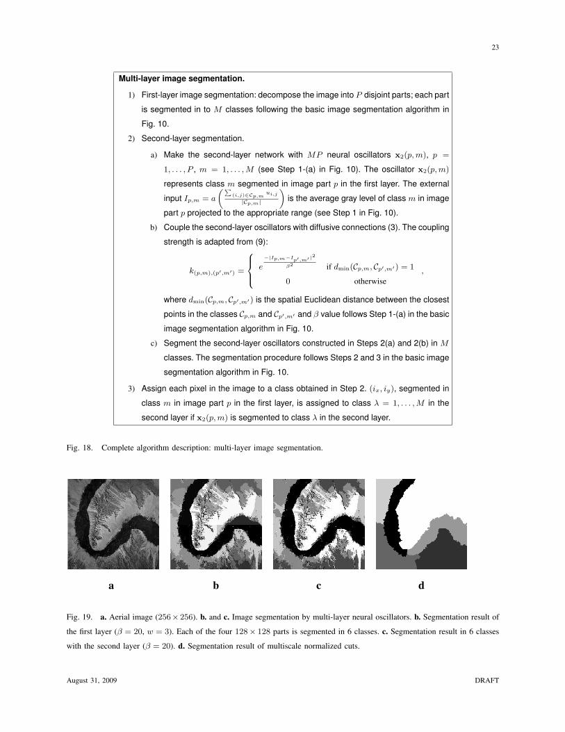
Fig. 19 illustrates an example of two-layer image segmentation. The image of size 256× 256

shown in Fig. 19-a is decomposed into four 128×128 parts. Fig. 19-b and c present respectively

the segmentation results of the first and second layers, both with 6 classes. From the first layer


22

Fig. 17. Two-layer image segmentation. In the first layer the image is decomposed into four disjoint parts. Each part is

segmented using the basic image segmentation algorithm. In the second layer one oscillator represents a class segmented in

the first layer, with the external input equal to the average gray-level in that class. Second-layer oscillators whose underlying

regions in the first layer are in vicinity are coupled.

to the second, some regions are merged, which corrects some over-segmentation and eliminates

some boundary artifacts in the first layer. The segmentation result in Fig. 19-c is satisfactory.

The river, although rather noisy in the original image, is segmented from the land with accurate

and regular boundary. The two aspects of the land are nicely segregated as well. The multiscale

normalized cuts segmentation [8] with the same number of classes shown in Fig. 19-d is less

delicate. While the land is segregated into coarse regions with some important details missing,

the river is over-segmented into two parts. Some river bank is confused with the river, which

results in the zigzag effect along the border of the river.

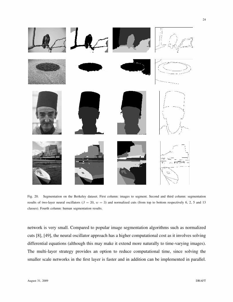
Fig. 20 shows the two-layer neural oscillators segmentation on some Berkeley benchmark

images (481× 321) [37], in comparison with the multiscale normalized cuts [8] and the human

segmentation results. While both neural oscillators and normalized cuts achieve rather satisfactory

segmentation, with the same number of classes the former seems to represent better important

detail structures and more pertinent to human performance.

To segment an image of size 128× 128, the basic neural oscillator solution implemented with

Matlab on a Pentium 4 PC takes between 10 and 30 minutes. The extra complexity due to

the feedback and the second layer in the multi-layer setting is marginal since the second-layer


23

Multi-layer image segmentation.

1) First-layer image segmentation: decompose the image into P disjoint parts; each part

is segmented in to M classes following the basic image segmentation algorithm in

Fig. 10.

2) Second-layer segmentation.

a) Make the second-layer network with MP neural oscillators x2(p, m), p =

1, . . . , P , m = 1, . . . , M (see Step 1-(a) in Fig. 10). The oscillator x2(p, m)

represents class m segmented in image part p in the first layer. The external

input Ip,m = a

(∑(i,j)∈Cp,m

ui,j

|Cp,m|

)is the average gray level of class m in image

part p projected to the appropriate range (see Step 1 in Fig. 10).

b) Couple the second-layer oscillators with diffusive connections (3). The coupling

strength is adapted from (9):

k(p,m),(p′,m′) =

e−|Ip,m−I

p′,m′ |2

β2 if dmin(Cp,m, Cp′,m′) = 1

0 otherwise,

where dmin(Cp,m, Cp′,m′) is the spatial Euclidean distance between the closest

points in the classes Cp,m and Cp′,m′ and β value follows Step 1-(a) in the basic

image segmentation algorithm in Fig. 10.

c) Segment the second-layer oscillators constructed in Steps 2(a) and 2(b) in M

classes. The segmentation procedure follows Steps 2 and 3 in the basic image

segmentation algorithm in Fig. 10.

3) Assign each pixel in the image to a class obtained in Step 2. (ix, iy), segmented in

class m in image part p in the first layer, is assigned to class λ = 1, . . . , M in the

second layer if x2(p, m) is segmented to class λ in the second layer.

Fig. 18. Complete algorithm description: multi-layer image segmentation.

a b c d

Fig. 19. a. Aerial image (256× 256). b. and c. Image segmentation by multi-layer neural oscillators. b. Segmentation result of

the first layer (β = 20, w = 3). Each of the four 128× 128 parts is segmented in 6 classes. c. Segmentation result in 6 classes

with the second layer (β = 20). d. Segmentation result of multiscale normalized cuts.


24

Fig. 20. Segmentation on the Berkeley dataset. First column: images to segment. Second and third column: segmentation

results of two-layer neural oscillators (β = 20, w = 3) and normalized cuts (from top to bottom respectively 6, 2, 5 and 13

classes). Fourth column: human segmentation results.

network is very small. Compared to popular image segmentation algorithms such as normalized

cuts [8], [49], the neural oscillator approach has a higher computational cost as it involves solving

differential equations (although this may make it extend more naturally to time-varying images).

The multi-layer strategy provides an option to reduce computational time, since solving the

smaller scale networks in the first layer is faster and in addition can be implemented in parallel.


25

VI. CONCLUDING REMARKS

Inspired by neural synchronization mechanisms in perceptual grouping, simple networks of

neural oscillators coupled with diffusive connections have been proposed to implement visual

grouping problems. Stable multi-layer algorithms and feedback mechanisms have also been

studied. Compared with state-of-the-art approaches, the same algorithm has been shown to

achieve promising results on several classical visual grouping problems, including point cluster-

ing, contour integration, and image segmentation. As in any algorithm based on the simulation

of a large network of dynamical systems, our visual grouping algorithm by neural oscillators

has a relatively high computational complexity. Implementation with parallel computing systems

such as VLSI (very-large-scale integration) or GPU (graphic processing unit) will be useful for

extensive acceleration [17].

Acknowledgements

We would like to thank the anonymous reviewers for their pointed and constructive suggestions

for improving the paper.

APPENDIX

Appendix: Convergence and Stability

One can verify ([45], to which the reader is referred for more details on the analysis tools) that

a sufficient condition for global exponential concurrent synchronization of an oscillator network

is

λmin(VLVT ) > supa,t

λmax

(∂f

∂x(a, t)

), (10)

where λmin(A) and λmax(A) are respectively the smallest and largest eigenvalues of the sym-

metric matrix As = (A + AT )/2, L is the Laplacian matrix of the network (Lii =∑

j 6=i kij ,

Lij = −kij for j 6= i) and V is a projection matrix on M⊥. Here M⊥ is the subspace orthogonal

to the subspace M in which all the oscillators are in synchrony − or, more generally in the

case of a hierarchy, where all oscillators at each level of the hierarchy are in synchrony (i.e.,

x1 = · · · = xN at each level). Note that M itself need not be invariant (i.e. all oscillators


26

synchronized at each level of the hierarchy need not be a particular solution of the system), but

only needs to be a subspace of the actual invariant synchronization subspace ([19], [45] section

3.3.i.), which may consist of synchronized subgroups according to the input image. Indeed, the

space where all xi are equal (or, in the case of a hierarchy, where at each level all xi are

equal), while in general not invariant, is always a subspace of the actual invariant subspace

corresponding to synchronized subgroups.

These results can be applied e.g. to individual oscillator dynamics of the type (1). Let Ji denote

the Jacobian matrix of the individual oscillator dynamics (1), Ji = ∂[vi wi]T /∂[vi, wi]

T . Using

a diagonal metric transformation Θ = diag(√

cαβ, 1), one easily shows, similarly to [59], [60],

that the transformed Jacobian matrix ΘJiΘ−1−diag(k, 0) is negative definite for k > 3+ αβ

4.

More general forms of oscillators can also be used. For instance, other second-order models can

be created based on a smooth function f(.) and an arbitrary sigmoid-like function σ(.) ≥ 0 such

that 0 ≤ σ′(.) ≤ 1 , in the form

vi = f(vi)− wi + Ii (11)

wi = c[ασ(βvi)− wi] (12)

with the transformed Jacobian matrix negative definite for k > f ′(vi) + αβ4

.

From a stability analysis point of view, the coupling matrix K of the Gaussian-tuned coupling,

composed of coupling coefficients kij in (4), presents desirable properties. It is symmetric, and

the classical theorem of Schoenberg (see [39]) shows that it is positive definite. Also, although it

may actually be state-dependent, the coupling matrix K can always be treated simply as a time-

varying external variable for stability analysis and Jacobian computation purposes, as detailed

in ([59], section 4.4, [45], section 2.3).

REFERENCES

[1] G. Aubert and P. Kornprobst. Mathematical Problems in Image Processing: Partial Differential Equations and the Calculus

of Variations. Springer; 2nd ed. edition, 2006.

[2] G.J. Brown and D.L. Wang. Modelling the perceptual segregation of double vowels with a network of neural oscillators.

Neural Networks, 10(9):1547–1558, 1997.

[3] A. Buades, B. Coll, and J.M. Morel. A review of image denoising algorithms, with a new one. Multiscale Modeling &

Simulation, 4(2):490–530, 2005.


27

[4] G. Buzsaki. Rhythms of the Brain. Oxford University Press, USA, 2006.

[5] K. Chen and D.L. Wang. A dynamically coupled neural oscillator network for image segmentation. Neural Networks,

15(3):423–439, 2002.

[6] Y. Cheng. Mean Shift, Mode Seeking, and Clustering. Pattern Analysis and Machine Intelligence, IEEE Transactions on,

page 790799, 1995.

[7] D. Comaniciu and P. Meer. Mean Shift: A Robust Approach Toward Feature Space Analysis. Pattern Analysis and Machine

Intelligence, IEEE Transactions on, pages 603–619, 2002.

[8] T.B. Cour, F. Benezit, and J. Shi. Spectral Segmentation with Multiscale Graph Decomposition. In Computer Vision and

Pattern Recognition, 2005. CVPR 2005. IEEE Computer Society Conference on, volume 2, 2005.

[9] A. Desolneux, L. Moisan, and J.-M. Morel. Computational gestalts and perception thresholds. Journal of Physiology -

Paris, 97(2-3):311–322, 2003.

[10] A. Desolneux, L. Moisan, and J.-M. Morel. A grouping principle and four applications. IEEE Transactions on Pattern

Analysis and Machine Intelligence, 25(4):508–513, 2003.

[11] A. Desolneux, L. Moisan, and J.-M. Morel. Gestalt Theory and Image Analysis, a Probabilistic Approach.

Interdisciplinary Applied Mathematics series, Springer Verlag, 2007. Preprint available at http://www.cmla.ens-

cachan.fr/Utilisateurs/morel/lecturenote.pdf.

[12] A. Desolneux P. Mus F. Cao, J. Delon and F. Sur. A unified framework for detecting groups and application to shape

recognition. Technical Report 1746, IRISA, September 2005.

[13] O. Faugeras, F. Grimbert, and J.J. Slotine. Stability and synchronization in neural fields. S.I.A.M. Journal on Applied

Mathematics, 68(8), 2008.

[14] D. J. Field, A. Hayes, and R. F. Hess. Contour integration by the human visual system: evidence for a local ”association

field”. Vision Res, 33(2):173–193, January 1993.

[15] R. FitzHugh. Impulses and physiological states in theoretical models of nerve membrane. Biophysical Journal, 1:445–466.,

1961.

[16] K. Fukunaga and L. Hostetler. The estimation of the gradient of a density function, with applications in pattern recognition.

Information Theory, IEEE Transactions on, 21(1):32–40, 1975.

[17] D. Geiger and F. Girosi. Parallel and deterministic algorithms from MRFs: surfacereconstruction. Pattern Analysis and

Machine Intelligence, IEEE Transactions on, 13(5):401–412, 1991.

[18] S. Geman and D. Geman. Stochastic relaxation, Gibbs distributions and the Bayesian restoration of images. Readings in

Computer Vision: Issues, Problems, Principles, and Paradigms, pages 564–584, 1987.

[19] L. Gerard and J.J.E. Slotine. Neuronal networks and controlled symmetries. arXiv:q-bio/0612049v4.

[20] L. Grady. Space-Variant Computer Vision: A Graph-Theoretic Approach. PhD thesis, Boston University Graduate School

of Arts and Sciences, 2004.

[21] J. Hawkins and S. Blakeslee. On Intelligence, 2004.

[22] J Hawkins and S Blakeslee. On Intelligence. Holt Paperbacks, 2005.

[23] R.F. Hess, A. Hayes, and DJ Field. Contour integration and cortical processing. Journal of Physiology-Paris, 97(2-3):105–

119, 2003.

[24] E.R. Kandel, J.J. Schwartz, and T.M. Jessel. Principles of Neural Science, 4th Edition. McGraw-Hill, New York, 2000.

[25] G. Kanizsa. Grammatica del Vedere, Il Mulino, Bologna, 1980. Traduction francaise: La grammaire du voir, Diderot

Editeur, Arts et Sciences, 1996.


28

[26] M. Kuzmina, E. Manykin, and I. Surina. Tunable Oscillatory Network for Visual Image Segmentation. Proc. of ICANN,

pages 1013–1019, 2001.

[27] M. Kuzmina, E. Manykin, and I. Surina. Oscillatory network with self-organized dynamical connections for

synchronization-based image segmentation. BioSystems, 76(1-3):43–53, 2004.

[28] T.S. Lee. Computations in the early visual cortex. Journal of Physiology-Paris, 97(2-3):121–139, 2003.

[29] Z. Li. A Neural Model of Contour Integration in the Primary Visual Cortex. Neural Computation, 10(4):903–940, 1998.

[30] Z. Li. Visual segmentation by contextual influences via intra-cortical interactions in the primary visual cortex. Network:

Computation in Neural Systems, 10(2):187–212, 1999.

[31] Z. Li. Pre-attentive segmentation in the primary visual cortex. Spatial Vision, 13(1):25–50, 2000.

[32] Z. Li. Computational Design and Nonlinear Dynamics of a Recurrent Network Model of the Primary Visual Cortex*.

Neural Computation, 13(8):1749–1780, 2001.

[33] X. Liu and D.L. Wang. Range image segmentation using a relaxation oscillator network. Neural Networks, IEEE

Transactions on, 10(3):564–573, 1999.

[34] X. Liu and D.L. Wang. A spectral histogram model for texton modeling and texture discrimination. Vision Research,

42(23):2617–2634, 2002.

[35] X. Liu and D.L. Wang. Image and texture segmentation using local spectral histograms. IEEE Transactions on Image

Processing, 15(10):3066, 2006.

[36] S. Mallat. Geometrical grouplets. Applied and Computational Harmonic Analysis, 2008.

[37] D. Martin, C. Fowlkes, D. Tal, and J. Malik. A database of human segmented natural images and its application to evaluating

segmentation algorithms and measuring ecological statistics. In Proc. 8th Int’l Conf. Computer Vision, volume 2, pages

416–423, July 2001.

[38] W. Metzger. Laws of seeing. 2006.

[39] C.A. Micchelli. Interpolation of scattered data: Distance matrices and conditionally positive definite functions. Constructive

Approximation, (2):11–22, 1986.

[40] J.M. Morel and S. Solimini. Variational methods in image segmentation. Progress in Nonlinear Differential Equations

and their Applications, 14, 1995.

[41] D. Mumford and J. Shah. Optimal approximations by piecewise smooth functions and associated variational problems.

Comm. Pure Appl. Math, 42(5):577–685, 1989.

[42] J. Nagumo, S. Arimoto, and S. Yoshizawa. An active pulse transmission line simulating nerve axon. Proceedings of the

IRE, 50(10):2061–2070, Oct. 1962.

[43] Edwin Olson, Matthew Walter, John Leonard, and Seth Teller. Single cluster graph partitioning for robotics applications.

In Proceedings of Robotics Science and Systems, pages 265–272, 2005.

[44] P. Perona and W. Freeman. A factorization approach to grouping. European Conference on Computer Vision, 1:655–670,

1998.

[45] Q.C. Pham and J.J. Slotine. Stable concurrent synchronization in dynamic system networks. Neural Netw., 20(1):62–77,

2007.

[46] U. Polat and D. Sagi. Lateral Interactions between Spatial Channels: Suppression and Facilitation Revealed by Lateral

Masking Experiments. Vision Research, 33:993–999, 1992.

[47] R.P.N. Rao and D.H. Ballard. Predictive coding in the visual cortex: a functional interpretation of some extra-classical

receptive-field effects. Nature Neuroscience, 2:79–87, 1999.


29

[48] T. Serre, L. Wolf, S. Bileschi, M. Riesenhuber, and T. Poggio. Robust Object Recognition with Cortex-Like Mechanisms.

IEEE Transaction On Pattern Analysis and Machine Intelligence, pages 411–426, 2007.

[49] J. Shi and J. Malik. Normalized Cuts and Image Segmentation. IEEE Transaction On Pattern Analysis and Machine

Intelligence, pages 888–905, 2000.

[50] W. Singer and C.M. Gray. Visual Feature Integration and the Temporal Correlation Hypothesis. Annual Reviews in

Neuroscience, 18(1):555–586, 1995.

[51] E. Sudderth and M.I. Jordan. Shared segmentation of natural scenes using dependent Pitman-Yor processes. Advances in

Neural Information Processing Systems, 21, 2009.

[52] D. Terman and D.L. Wang. Global competition and local cooperation in a network of neural oscillators. Physica D:

Nonlinear Phenomena, 81(1-2):148–176, 1995.

[53] S. Ullman and A. Shashua. Structural Saliency: The Detection of Globally Salient Structures Using a Locally Connected

Network. ICCV, Clearwater, FL, 1988.

[54] D.L. Wang. The time dimension for scene analysis. Neural Networks, IEEE Transactions on, 16(6):1401–1426, 2005.

[55] D.L. Wang and G.J. Brown. Separation of speech from interfering sounds based on oscillatorycorrelation. Neural Networks,

IEEE Transactions on, 10(3):684–697, 1999.

[56] D.L. Wang and P. Chang. An oscillatory correlation model of auditory streaming. Cognitive Neurodynamics, 2(1):7–19,

2008.

[57] D.L. Wang and D. Terman. Locally excitatory globally inhibitory oscillator networks. Neural Networks, IEEE Transactions

on, 6(1):283–286, 1995.

[58] D.L. Wang and D. Terman. Image Segmentation Based on Oscillatory Correlation. Neural Computation, 9(4):805–836,

1997.

[59] W. Wang and J.J.E. Slotine. On partial contraction analysis for coupled nonlinear oscillators. Biological Cybernetics,

92(1):38–53, 2005.

[60] W. Wang and J.J.E. Slotine. Contraction analysis of time-delayed communications and group cooperation. IEEE

Transactions on Automatic Control,, 51(4):712– 717, 2006.

[61] R.J. Watt and W.A. Phillips. The function of dynamic grouping in vision. Trends in Cognitive Sciences, 4(12):447–454,

2000.

[62] M. Wertheimer. Untersuchungen zur Lehre der Gestalt, II. Psychologische Forschung, 4:301–350, 1923. Translation

published as Laws of Organization in Perceptual Forms, in Ellis, W. (1938). A source book of Gestalt psychology (pp.

71-88). Routledge & Kegan Paul.

[63] S.C. Yen and L.H. Finkel. Extraction of perceptually salient contours by striate cortical networks. Vision Research,

38(5):719–741, 1998.


Documents

1 Visual Grouping by Neural Oscillator Networks - MITweb.mit.edu/nsl/www/preprints/visual_oscillators.pdf · Visual Grouping by Neural Oscillator Networks ... State-of-the-art visual