Embed Size (px)
Citation preview

1
Verification & Validation

2
Motivation
The simulation model needs to work as intended.It should adequately represent the system being simulated.

3
Verification & Validation
Verification –
Validation –

4
Verification
Possible methods
…
Use all of the prior methods in extreme cases Examples
Examine only one part type at a time. Allow only one entity into the system.

5
Verification
Use all of the prior methods in extreme cases Examples
Control the distributions used. Set all processing times to constants – You should be
able to predict quantities such as the entity avg. TIS. Control arrival rates
Extremely high. Extremely low.

6
Verification
Need to run very large models for a long simulated time to check for gradual buildup of queues.
May be able to compute utilizations.
During model development

7
Validation
In general this is more difficult than verification.Two general cases

8
Validation
System exists. Compare results to historical results.
Does the data exist? Are you comparing “apples to apples”?
Control model variability Resource availability
If a known long maintenance period occurred for machines or if known long failures/repairs occurred, duplicate these in the model.
Duplicate resource schedules. Duplicate the arrival pattern over which historical
performance data has been collected. Job types. Job arrival times.

9
Validation
System does not exist. Change the data and modify the model so that it
simulates a system that still exists. Then compare to historical data.
Expert opinion. Run extreme cases.
10
Output Analysis

11
Introduction
A simulation model has been constructed of a system to generate estimates of one or more performance measures.Random inputs/system components in the simulation imply that the outputs (performance measure estimates) will be observations from probability distributions.

12
Introduction
Questions about starting and running the model.

13
Types of Simulation “Runs”
In general, there are two types of simulation analyses performed that dictate how the previous questions should be answered.
1. Terminating –
2. Steady state –

14
Example
Simulation of a bank from open to close (9AM-5PM).
This is an example of a terminating simulation. How do you start the simulation?
Empty and idle. How long should the model be run (how much
simulated time before stopping the run)? 9AM until all customers depart after 5PM.

15
Terminating Simulations
Time period of interest is defined.

16
ExampleBank simulation from 9AM-5PM.
Customers arriving before 5PM are all served. The simulation ending time may vary from replication
to replication. What is the termination criteria?

17
Arena
To properly end such a simulation, use Run -> Setup -> Replication Parameters
1. Set ending criteria in “Terminating Condition”.2. Leave “Replication Length” field blank.
The termination criteria will use Arena “syntax”.

18
Arena

19
Terminating Simulations
A simulation of a service facility with “rush hour” periods is constructed. There is a specific time period of interest – 11AM -1PM. The facility is open at 9AM.
How long to simulate? 11AM-1PM.

20
Terminating Simulations
Approaches for starting a simulation with unknown initial conditions.
1. Collect data on the system state at the start of the rush hour period. Initialize the simulation with the “average” system
state. Initialize the simulation with a random system
state based on the collected data. Both hard to do in Arena, Straightforward in an “event driven” model (e.g., the
manual simulation).

21
Terminating Simulations
Approaches for starting a simulation with unknown initial conditions.
2.

22
Arena

23
Steady State Simulations
Steady state simulations are used to understand how a system performs after being in operations for a long time. The system has reached “steady state” where the performance is independent of the initial conditions.Examples
Production line simulations – the line starts where it left off at the end of prior shifts.
Emergency rooms. Worst case analysis.

24
Steady State Simulations
How to start the simulation? Typically a warm-up period is used to minimize any
impact of initial conditions. How long should the warm-up period be?
Can determine from some sample runs of the simulation.
How long to run the simulation? Can determine from some sample runs of the
simulation.

25
Steady State Simulations

26
Steady State Simulations
What are you looking for in the plots? Impact of initial conditions.
Does the plot from time zero look different than other portions of the graph?
Does the performance measure seem to be growing without bound?

27
The Number of Replications and Analysis of Output
We will focus on the analysis of terminating simulations.
They are more common in practice. The analysis is more straightforward.
Simulation models are used for experimentation.
One simulation replication → a single realization of each system performance measure.
n independent replications → n independent samples from the same distribution.

28
The Number of Replications and Analysis of Output
Consider a single performance measure. Let Xi be the random variable that represents the value of the performance measure for the ith simulation replication. xi = outcome/realization of Xi from the ith simulation
replication.
Since the Xi are independent and identically distributed random variables the performance can be characterized using the “typical” confidence interval.

29
Analysis of OutputThe approximate confidence interval
Assumes the observations are from a normal distribution.
%100*)1(

30
The Number of ReplicationsHow to estimate number of independent replications required for a desired precision expressed as a confidence interval half-width.
The half-width h of this confidence interval is
This cannot be used to precisely calculate n to get the desired precision h since the t-value is a function of n.

31
The Number of ReplicationsSubstitute
Use this formula to approximate the number of replications needed to get a desired half-width (precision) for some performance measure.

32
Example – Average Time In System (TIS) for entities being processed.
The Number of Replications

33
The Number of Replications
Use Arena to send TIS average results from independent replications to a text file.
Use this data to estimate n – the number of independent replications needed for a desired precision.

34
The Number of Replications

35
The Number of ReplicationsProject: Exercise 3.1User: KeltonData item: TIS2Run date: 2/27/2006Options: YDT 20
Time Observation1 8.341297
-1 02 7.39797
-2 03 5.40304
-3 04 9.393243
-4 05 3.859661
-5 06 14.76574
-6 07 26.15339
-7 0

36
The Number of Replications
2
22
2/1
2/1,12/1
)A(*
for
h
vgTISszn
tz n
4535.
43.596.1
96.1
2
22
025.01
n
z
Avg. 8.187022Stdev 5.428285
37
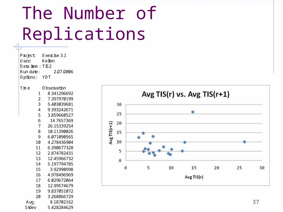
The Number of Replications
Project: Exercise 3.1User: KeltonData item: TIS2Run date: 2/27/2006Options: YDT
Time Observation1 8.3412966922 7.3979701993 5.4030396814 9.3932426715 3.8596605276 14.76573697 26.153392548 10.113900269 6.071090565
10 4.27843690411 6.39067732812 2.87478243113 12.4596673214 5.19779478515 3.9299099816 4.97849696917 6.02967206418 12.9957467919 9.83705107220 3.268866729
Avg. 8.18702162Stdev 5.428284629

38
Comparing Two Alternatives
In many situations where simulation is used, changes to an existing or “base” system are explored.There is a need to do a comparison of two systems.Simulation has been used to generate estimates of performance measure for the base system and a changed system.Analysis
Two sample t-confidence interval. Paired t-confidence interval.

39
Comparing Two Alternatives
control). is h there(over whic conducted weresexperimentsimulation thehowon depends and of ceindependen The
)(
.21for model) simulation theof 1n replicatio from TIS average theis (e.g.,
measure eperformanc system some of nsobservatio ddistributeyidenticall andt independen of sample a be ,,,
Let
21
21
1
21
jj
iji
i
iiinii
XX
XE
,iX
nXXX

40

41

42
Comparing Two Alternatives
“Standard” two-sample t-confidence interval.Assumptions X1j’s and X2j’s are independent.
Var(X1j) = Var(X2j) .
n1 and n2 need not be equal.
Not recommended for simulation output analysis since the equal variance assumption is often not met (Kelton and Law 2000).
However, the test is robust if n1 = n2.

43
Comparing Two Alternatives
“Welch” two-sample t-confidence interval.Assumptions X1j’s and X2j’s are independent and normally
distributed. n1 and n2 need not be equal.

44
Comparing Two Alternatives
222211
212/1,ˆ2211
22
22221
211
21
222
2211
21
2221
212211
/)(/)()()(
as interval confidence theForm
)1/(]/)([)1/(]/)([
]/)(/)([ˆ
ˆ freedom of degrees estimated theCompute
).(),(),(),(
s,simulation two theofoutput for the variancessample and means sample Compute
nnsnnstnXnX
nnnsnnns
nnsnnsf
f
nsnsnXnX
f

45
Comparing Two Alternatives
Paired t-confidence interval.Assumptions
n1 and n2 are equal.

46
Comparing Two Alternatives
n
DstnD
Dsn
D
nD
XXD
jn
j
n
jj
jjj
)()(
:is interval confidence The
variance.sample )( ,)(
)(
Let
2
2/1,1
21
21

47
Comparing Two Alternatives
The paired t-confidence interval forms a new sample as the difference between corresponding outputs from the same replication number for system 1 and system 2. X1j and X2j may be dependent.
The Di’s must be independent.
Var(X1j) = Var(X2j) is not necessary.

48
Example
Experiment with the single server model arrival process.
t 9,.975 = 2.26, Performance measure is avg. TIS.Time Expo(5) U(1,9) D1 8.341 8.328 0.0132 7.398 6.228 1.1703 5.403 5.943 -0.5404 9.393 7.924 1.4695 3.860 2.475 1.3856 14.766 8.086 6.6797 26.153 12.673 13.4808 10.114 15.218 -5.1049 6.071 5.893 0.178
10 4.278 4.161 0.117Avg. 1.885Stdev. 4.974

49
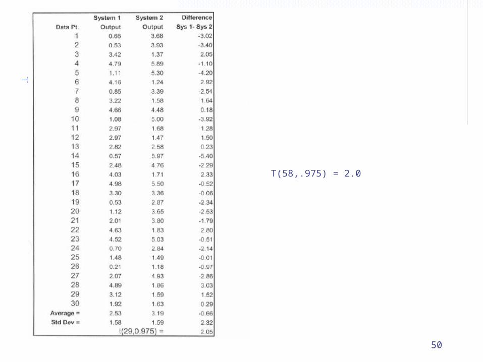
In-class ExerciseFor the following data.
Form 95% CIs for system 1 and system 2 output separately. Check for overlap.
Form a 95% paired t-confidence interval. Check for the inclusion of zero.
Construct a Welch two-sample t-confidence interval.
222211
212/1,ˆ2211
22
22221
211
21
222
2211
21
/)(/)()()(
as interval confidence theForm
)1/(]/)([)1/(]/)([
]/)(/)([ˆ
nnsnnstnXnX
nnnsnnns
nnsnnsf
f
n
DstnD
Dsn
D
nD
XXD
jn
j
n
jj
jjj
)()(
:is interval confidence The
variance.sample )( ,)(
)(
Let
2
2/1,1
21
21
50
T(58,.975) = 2.0

51
In-class Exercise

52

53
Comparing >2 SystemsComparisons with a base system.All pairwise comparisons.Simple procedure is to apply what is called the Bonferroni inequality.
k
jjj kjCI
1
1),,2,1 allfor , valueProb(True

54
Comparing >2 SystemsExample – One base system and four alternatives => four confidence intervals when comparing each system with the base system.To get 90% overall confidence level each individual confidence interval should be a 97.5% CI.
ci /1

55
Comparing >2 SystemsExperimental design methods are helpful for exploring a “factor space”.Care must be taken when conducting the experiments and analyzing experimental results due to the non-random nature of generating “random” values in a simulation.