1 Validation of Large-Eddy Simulation Methods for Gravity

Validation of Large-Eddy Simulation Methods for Gravity-Wave Breaking1

Sebastian Remmler∗ and Stefan Hickel† ‡2

Institute of Aerodynamics and Fluid Mechanics, Technische Universitat Munchen, Germany.3

Mark D. Fruman and Ulrich Achatz4

Institute for Atmosphere and Environment, Goethe-University Frankfurt, Germany.5

∗Current affiliation: AUDI AG, I/EK-44, 85045 Ingolstadt, Germany.6

†Current affiliation: Delft University of Technology, The Netherlands.7

‡Corresponding author address: Stefan Hickel, Department of Aerospace Engineering, Delft Uni-

versity of Technology, Kluyverweg 1, 2629 HS Delft, The Netherlands.

8

9

E-mail: [email protected]

Generated using v4.3.2 of the AMS LATEX template 1

ABSTRACT

In order to reduce the computational costs of numerical studies of gravity

wave breaking in the atmosphere, the grid resolution has to be reduced as

much as possible. Insufficient resolution of small-scale turbulence demands

a proper turbulence parametrisation in the framework of large-eddy simula-

tion (LES). We validate three different LES methods – the Adaptive Local

Deconvolution Method (ALDM), the dynamic Smagorinsky method (DSM)

and a naıve central discretisation without turbulence parametrisation (CDS4)

– for three different cases of the breaking of well defined monochromatic

gravity waves. For ALDM we developed a modification of the numerical flux

functions that significantly improves the simulation results in case of a tem-

porarily very smooth velocity field. The test cases include an unstable and

a stable inertia-gravity wave as well as an unstable high-frequency gravity

wave. All simulations are carried out both in three-dimensional domains and

in two-dimensional domains in which the velocity and vorticity fields are three

dimensional (so-called 2.5-D simulations). We find that results obtained with

ALDM and DSM are generally in good agreement with the reference direct

numerical simulations as long as the resolution in the direction of the wave

vector is sufficiently high. The resolution in the other directions has a weaker

influence on the results. The simulations without turbulence parametrisation

are only successful if the resolution is high and the level of turbulence com-

paratively low.

11

12

13

14

15

16

17

18

19

20

21

22

23

24

25

26

27

28

29

30

31

2

1. Introduction32

Gravity waves are a common phenomenon in any stably stratified fluid, such as the atmosphere33

of the earth. They can be excited by flow over orography (e.g. Smith 1979; McFarlane 1987), by34

convection (e.g. Chun et al. 2001; Grimsdell et al. 2010), and by spontaneous imbalance of the35

mean flow in the troposphere (O’Sullivan and Dunkerton 1995; Plougonven and Snyder 2007).36

Gravity waves transport energy and momentum from the region where they are forced to the re-37

gion where they are dissipated (e.g. through breaking), possibly far away from the source region.38

Various phenomena, such as the cold summer mesopause (Hines 1965) and the quasi-biennial39

oscillation in the equatorial stratosphere (e.g. Baldwin et al. 2001), cannot be explained nor repro-40

duced in weather and climate simulations without accounting for the effect of gravity waves. See41

Fritts and Alexander (2003) for an overview of gravity waves in the middle atmosphere. Prusa42

et al. (1996) found in numerical experiments that (due to wave dispersion) gravity waves gener-43

ated in the troposphere at a broad wavelength spectrum reach the upper mesosphere as an almost44

monochromatic wave packet with a horizontal wavelength between a few kilometres and more45

than 100 km, depending on the horizontal scale of the forcing and the background conditions.46

Since most gravity waves have a wavelength that is not well resolved in general circulation mod-47

els, the effect of gravity waves on the global circulation is usually accounted for by parametrisation48

based on combinations of linear wave theory (Lindzen 1981), empirical observations of time-mean49

energy spectra (e.g. Hines 1997), and simplified treatments of the breaking process. See Kim et al.50

(2003) and McLandress (1998) for reviews of the various standard parametrisation schemes.51

A common weakness of most parametrisation schemes is the over-simplified treatment of the52

wave breaking process. Improving this point requires a deeper insight into the breaking process53

that involves generation of small scale flow features through wave-wave interactions and through54

3

wave-turbulence interactions. Since the gravity-wave wavelength and the turbulence that even-55

tually leads to energy dissipation into heat span a wide range of spatial and temporal scales, the56

breaking process is challenging both for observations and numerical simulations. Direct Numeri-57

cal Simulations (DNS) must cover the breaking wave with a wavelength of a few kilometres as well58

as the smallest turbulence scales (the Kolmogorov length η). The Kolmogorov length depends on59

the kinetic energy dissipation and the kinematic viscosity. It is on the order of millimetres in the60

troposphere (Vallis 2006) and approximately 1 m at 80 km altitude (Remmler et al. 2013).61

The necessity of resolving the Kolmogorov scale can be circumvented by applying the approach62

of Large-Eddy Simulation (LES), i.e. by parametrising the effect of unresolved small eddies on63

the resolved large-scale flow.64

This can be necessary in cases where DNS would be too expensive, e.g. in investigating the65

dependence of the gravity wave breaking on several parameters (propagation angle, wavelength,66

amplitude, viscosity, stratification) at the same time; for problems in which many wavelengths67

need to be resolved – such as propagation of a wave packet or wave train through a variable68

background (Lund and Fritts 2012) or modelling realistic cases of waves generated by topography69

or convection; for validating quasilinear wave-propagation theory (Muraschko et al. 2014); or for70

validating gravity-wave-drag parametrisation schemes.71

The subgrid-scale parametrisation of turbulence is, of course, a source of uncertainty and, where72

possible, should be validated against fully resolved DNS or observations for every type of flow73

for which it is to be used. Many numerical studies of breaking gravity waves rely on the LES74

principle without such a validation (e.g. Winters and D’Asaro 1994; Lelong and Dunkerton 1998;75

Andreassen et al. 1998; Dornbrack 1998; Afanasyev and Peltier 2001).76

Recent studies (Fritts et al. 2009, 2013; Fritts and Wang 2013) have presented highly resolved,77

high Reynolds number DNS of a monochromatic gravity wave breaking. However, they do not78

4

take into account the Coriolis force, which has a large influence on the dynamics of breaking79

for low-frequency gravity waves (Dunkerton 1997; Achatz and Schmitz 2006b), often referred80

to as inertia-gravity waves (IGWs) as opposed to high-frequency gravity waves (HGWs). The81

Coriolis force induces an elliptically polarised transverse velocity field in IGWs, and the velocity82

component normal to the plane of propagation of the wave has its maximum shear at the level83

of minimum static stability. Dunkerton (1997) and Achatz and Schmitz (2006b) showed that this84

strongly influences the orientation of the most unstable perturbations.85

An important aspect in setting up a simulation of a gravity wave breaking event is the proper86

choice of the domain size and initial conditions. While the gravity wave itself depends on one87

spatial coordinate and has a natural length scale given by its wavelength, the breaking process88

and the resulting turbulence is three-dimensional and proper choices have to be made for the do-89

main sizes in the two directions perpendicular to the wave vector. Achatz (2005) and Achatz and90

Schmitz (2006a) analysed the primary instabilities of monochromatic gravity waves of various am-91

plitudes and propagation directions using normal-mode and singular-vector analysis, and Fruman92

and Achatz (2012) extended this analysis for IGWs by computing the leading secondary singu-93

lar vectors with respect to a time-dependent simulation of the perturbed wave. (Normal-mode94

analysis is not suited to time-dependent basic states, while singular-vector analysis, whereby the95

perturbations whose energy grows by the largest factor in a given optimisation time, is always pos-96

sible.) They found that the wavelength of the optimal secondary perturbation can be much shorter97

than the wavelength of the original wave. Thus the computational domain for a three-dimensional98

simulation need not necessarily have the size of the base wavelength in all three directions. They99

proposed the following multi-step approach to set-up the domain and initial conditions for a DNS100

of a given monochromatic gravity wave:101

5

1. solution (in the form of normal modes or singular vectors) of the governing (Boussinesq)102

equations linearised about the basic state wave, determining the primary instability structures;103

2. two-dimensional (in space) numerical solution of the full nonlinear equations using the result104

of stage 1 as initial condition;105

3. solution in the form of singular vectors (varying in the remaining spatial direction) of the106

governing equations linearised about the time-dependent result of stage 2;107

4. three-dimensional DNS using the linear solutions from stages 1 and 3 as initial condition and108

their wavelengths for the size of the computational domain.109

This procedure was applied to an unstable IGW by Remmler et al. (2013) and fully elaborated110

with two additional test cases by Fruman et al. (2014).111

Having these properly designed DNS results available, we can now use them for the validation112

of computationally less expensive methods. Hence the present study analyses the suitability of113

different LES methods for the cases presented by Fruman et al. (2014), viz. an unstable IGW,114

a stable IGW and an unstable HGW, all of them with a base wavelength of 3 km. The first LES115

method to be applied is the Adaptive Local Deconvolution Method (ALDM) of Hickel et al. (2006,116

2014). It is an “implicit” LES method since the SGS stress parametrisation is implied in the117

numerical discretisation scheme. Based on ALDM for incompressible flows and its extension to118

passive scalar mixing (Hickel et al. 2008), Remmler and Hickel (2012, 2013); Rieper et al. (2013)119

successfully applied ALDM to stably stratified turbulent flows.120

For the present study, the numerical flux function for the active scalar in ALDM has been mod-121

ified to prevent the method from generating spurious oscillations in partially laminar flow fields.122

The second method to be applied is the the well known Smagorinsky (1963) method with the123

dynamic estimation of the spatially nonuniform model parameter proposed by Germano et al.124

6

(1991) and refined by Lilly (1992). The third LES method is a “naıve” approach with a simple125

central discretisation scheme and no explicit SGS parametrisation. This method is theoretically126

dissipation-free but can lead to numerical instability if the turbulence level is high (which was the127

reason for the development of the first explicit SGS parametrisation by Smagorinsky 1963). How-128

ever, the method is computationally inexpensive and can be used in some cases without problems,129

as we will show.130

We apply these methods to the three gravity-wave test cases using grids of different refinement131

levels with the goal of using as few grid cells as possible while still obtaining good agreement with132

the DNS results. We also run small ensembles for each simulation with only slightly different ini-133

tial conditions to get an estimate of the sensitivity and variability of the results. All this is done in134

a three dimensional domain (with the same domain size as the DNS) and in a two-dimensional do-135

main in which the two dimensions are chosen to be parallel to the wave vectors of the gravity wave136

and of the most important growing primary perturbation (without the addition of the secondary sin-137

gular vector, cf. step 2 above). Since the velocity and vorticity fields are three-dimensional and138

since the turbulent cascade is direct (energy moves to smaller length scales), these simulations are139

sometimes called “2.5-D”. Fruman et al. (2014) found that 2.5-D and 3-D results are broadly very140

similar for the inertia–gravity-wave test cases considered here.141

The paper is organised as follows. In section 2 the governing equations used for the simulations142

are presented along with properties of the inertia-gravity wave solutions and the energetics of the143

system. Section 3 describes the numerical methods used, in particular the three LES schemes.144

The three test cases are reviewed in section 4 and the results of the simulations are discussed in145

sections 5 to 7.146

7

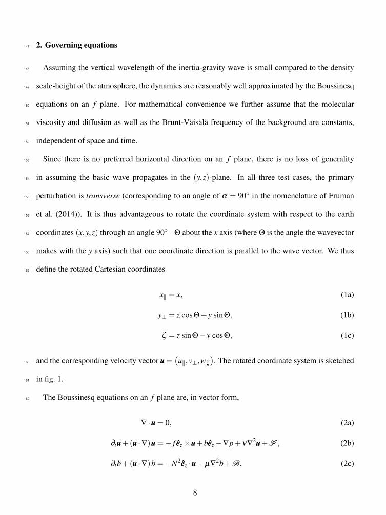
2. Governing equations147

Assuming the vertical wavelength of the inertia-gravity wave is small compared to the density148

scale-height of the atmosphere, the dynamics are reasonably well approximated by the Boussinesq149

equations on an f plane. For mathematical convenience we further assume that the molecular150

viscosity and diffusion as well as the Brunt-Vaisala frequency of the background are constants,151

independent of space and time.152

Since there is no preferred horizontal direction on an f plane, there is no loss of generality153

in assuming the basic wave propagates in the (y,z)-plane. In all three test cases, the primary154

perturbation is transverse (corresponding to an angle of α = 90◦ in the nomenclature of Fruman155

et al. (2014)). It is thus advantageous to rotate the coordinate system with respect to the earth156

coordinates (x,y,z) through an angle 90◦−Θ about the x axis (where Θ is the angle the wavevector157

makes with the y axis) such that one coordinate direction is parallel to the wave vector. We thus158

define the rotated Cartesian coordinates159

x‖ = x, (1a)

y⊥ = z cosΘ+ y sinΘ, (1b)

ζ = z sinΘ− y cosΘ, (1c)

and the corresponding velocity vector uuu =(u‖,v⊥,wζ

). The rotated coordinate system is sketched160

in fig. 1.161

The Boussinesq equations on an f plane are, in vector form,162

∇ ·uuu = 0, (2a)

∂tuuu+(uuu ·∇)uuu =− f eeez×uuu+beeez−∇p+ν∇2uuu+F , (2b)

∂tb+(uuu ·∇)b =−N2eeez ·uuu+µ∇2b+B, (2c)

8

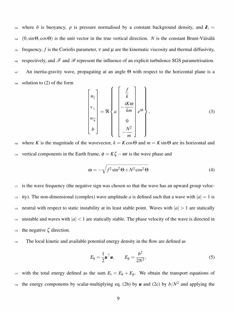
where b is buoyancy, p is pressure normalised by a constant background density, and eeez =163

(0,sinΘ,cosΘ) is the unit vector in the true vertical direction. N is the constant Brunt-Vaisala164

frequency, f is the Coriolis parameter, ν and µ are the kinematic viscosity and thermal diffusivity,165

respectively, and F and B represent the influence of an explicit turbulence SGS parametrisation.166

An inertia-gravity wave, propagating at an angle Θ with respect to the horizontal plane is a167

solution to (2) of the form168

u‖

v⊥

wζ

b

= ℜ

a

fk

− iKω

km

0

−N2

m

eiφ

, (3)

where K is the magnitude of the wavevector, k = K cosΘ and m = K sinΘ are its horizontal and169

vertical components in the Earth frame, φ = Kζ −ωt is the wave phase and170

ω =−√

f 2 sin2Θ+N2 cos2 Θ (4)

is the wave frequency (the negative sign was chosen so that the wave has an upward group veloc-171

ity). The non-dimensional (complex) wave amplitude a is defined such that a wave with |a|= 1 is172

neutral with respect to static instability at its least stable point. Waves with |a| > 1 are statically173

unstable and waves with |a|< 1 are statically stable. The phase velocity of the wave is directed in174

the negative ζ direction.175

The local kinetic and available potential energy density in the flow are defined as176

Ek =12

uuu>uuu, Ep =b2

2N2 , (5)

with the total energy defined as the sum Et = Ek + Ep. We obtain the transport equations of177

the energy components by scalar-multiplying eq. (2b) by uuu and (2c) by b/N2 and applying the178

9

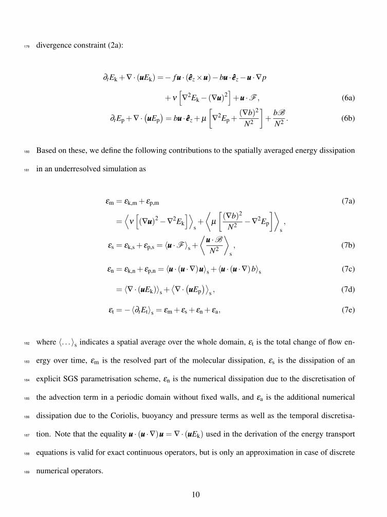
divergence constraint (2a):179

∂tEk +∇ · (uuuEk) =− fuuu · (eeez×uuu)−buuu · eeez−uuu ·∇p

+ν

[∇

2Ek− (∇uuu)2]+uuu ·F , (6a)

∂tEp +∇ ·(uuuEp)= buuu · eeez +µ

[∇

2Ep +(∇b)2

N2

]+

bB

N2 . (6b)

Based on these, we define the following contributions to the spatially averaged energy dissipation180

in an underresolved simulation as181

εm = εk,m + εp,m (7a)

=⟨

ν

[(∇uuu)2−∇

2Ek

]⟩s+

⟨µ

[(∇b)2

N2 −∇2Ep

]⟩s,

εs = εk,s + εp,s = 〈uuu ·F 〉s +⟨

uuu ·BN2

⟩s, (7b)

εn = εk,n + εp,n = 〈uuu · (uuu ·∇)uuu〉s + 〈uuu · (uuu ·∇)b〉s (7c)

= 〈∇ · (uuuEk)〉s +⟨∇ ·(uuuEp)⟩

s , (7d)

εt =−〈∂tEt〉s = εm + εs + εn + εa, (7e)

where 〈. . .〉s indicates a spatial average over the whole domain, εt is the total change of flow en-182

ergy over time, εm is the resolved part of the molecular dissipation, εs is the dissipation of an183

explicit SGS parametrisation scheme, εn is the numerical dissipation due to the discretisation of184

the advection term in a periodic domain without fixed walls, and εa is the additional numerical185

dissipation due to the Coriolis, buoyancy and pressure terms as well as the temporal discretisa-186

tion. Note that the equality uuu · (uuu ·∇)uuu = ∇ · (uuuEk) used in the derivation of the energy transport187

equations is valid for exact continuous operators, but is only an approximation in case of discrete188

numerical operators.189

10

3. Numerical methods190

a. The INCA model191

With our flow solver INCA, the Boussinesq equations are discretised by a fractional step method192

on a staggered Cartesian mesh. The code offers different discretisation schemes depending on the193

application, two of which are described below. For time advancement the explicit third-order194

Runge–Kutta scheme of Shu (1988) is used. The time-step is dynamically adapted to satisfy a195

Courant–Friedrichs–Lewy condition.196

The spatial discretisation is a finite-volume method. We use a 2nd order central difference197

scheme for the discretisation of the diffusive terms and for the pressure Poisson solver. The Pois-198

son equation for the pressure is solved at every Runge–Kutta sub step. The Poisson solver employs199

the fast Fourier-transform in the vertical (i.e. ζ ) direction and a Stabilised Bi-Conjugate Gradient200

(BiCGSTAB) solver (van der Vorst 1992) in the horizontal (x‖-y⊥) plane.201

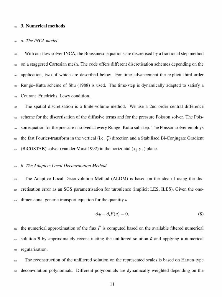
b. The Adaptive Local Deconvolution Method202

The Adaptive Local Deconvolution Method (ALDM) is based on the idea of using the dis-203

cretisation error as an SGS parametrisation for turbulence (implicit LES, ILES). Given the one-204

dimensional generic transport equation for the quantity u205

∂tu+∂xF(u) = 0, (8)

the numerical approximation of the flux F is computed based on the available filtered numerical206

solution u by approximately reconstructing the unfiltered solution u and applying a numerical207

regularisation.208

The reconstruction of the unfiltered solution on the represented scales is based on Harten-type209

deconvolution polynomials. Different polynomials are dynamically weighted depending on the210

11

smoothness of the filtered solution. The regularisation is obtained through a tailored numerical flux211

function operating on the reconstructed solution. Both the solution-adaptive polynomial weight-212

ing and the numerical flux function involve free model parameters that were calibrated in such213

a way that the truncation error of the discretised equations optimally represents the SGS stresses214

of isotropic turbulence (Hickel et al. 2006). This set of parameters was not changed for any sub-215

sequent applications of ALDM. For the presented computations, we used an implementation of216

ALDM with improved computational efficiency (Hickel and Adams 2007).217

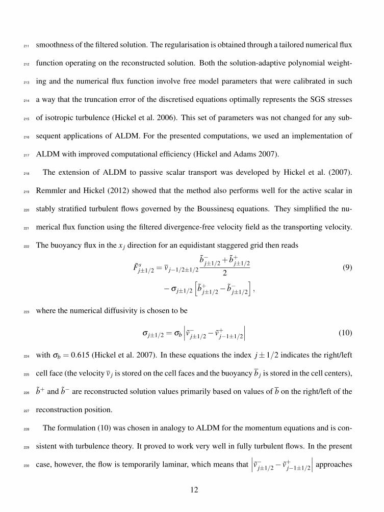
The extension of ALDM to passive scalar transport was developed by Hickel et al. (2007).218

Remmler and Hickel (2012) showed that the method also performs well for the active scalar in219

stably stratified turbulent flows governed by the Boussinesq equations. They simplified the nu-220

merical flux function using the filtered divergence-free velocity field as the transporting velocity.221

The buoyancy flux in the x j direction for an equidistant staggered grid then reads222

Fsj±1/2 = v j−1/2±1/2

b−j±1/2 + b+j±1/2

2(9)

−σ j±1/2

[b+j±1/2− b−j±1/2

],

where the numerical diffusivity is chosen to be223

σ j±1/2 = σb

∣∣∣v−j±1/2− v+j−1±1/2

∣∣∣ (10)

with σb = 0.615 (Hickel et al. 2007). In these equations the index j±1/2 indicates the right/left224

cell face (the velocity v j is stored on the cell faces and the buoyancy b j is stored in the cell centers),225

b+ and b− are reconstructed solution values primarily based on values of b on the right/left of the226

reconstruction position.227

The formulation (10) was chosen in analogy to ALDM for the momentum equations and is con-228

sistent with turbulence theory. It proved to work very well in fully turbulent flows. In the present229

case, however, the flow is temporarily laminar, which means that∣∣∣v−j±1/2− v+j−1±1/2

∣∣∣ approaches230

12

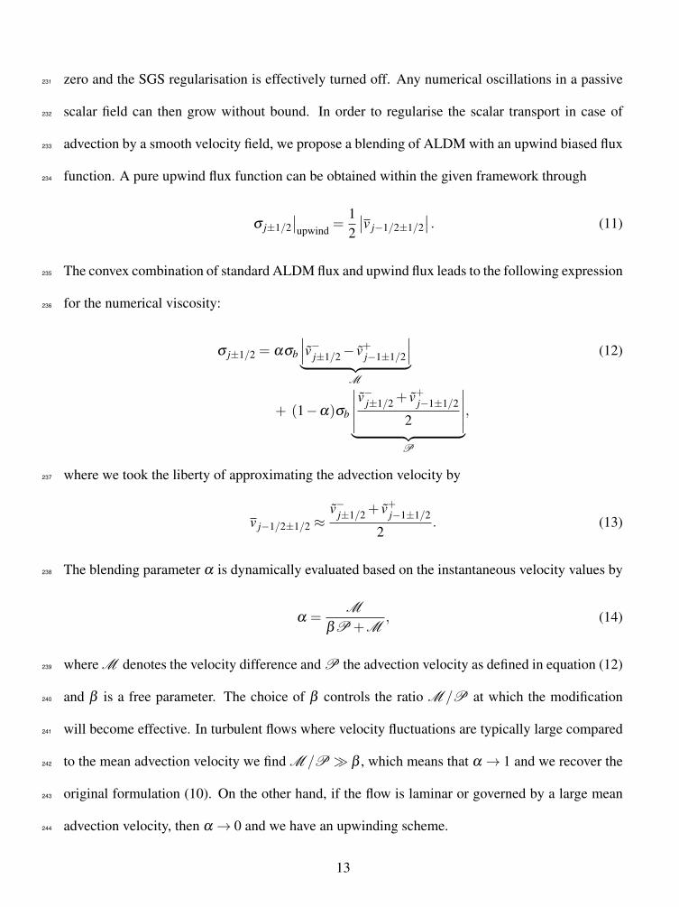
zero and the SGS regularisation is effectively turned off. Any numerical oscillations in a passive231

scalar field can then grow without bound. In order to regularise the scalar transport in case of232

advection by a smooth velocity field, we propose a blending of ALDM with an upwind biased flux233

function. A pure upwind flux function can be obtained within the given framework through234

σ j±1/2∣∣upwind =

12

∣∣v j−1/2±1/2∣∣ . (11)

The convex combination of standard ALDM flux and upwind flux leads to the following expression235

for the numerical viscosity:236

σ j±1/2 = ασb

∣∣∣v−j±1/2− v+j−1±1/2

∣∣∣︸︷︷︸M

(12)

+ (1−α)σb

∣∣∣∣∣ v−j±1/2 + v+j−1±1/2

2

∣∣∣∣∣︸︷︷︸P

,

where we took the liberty of approximating the advection velocity by237

v j−1/2±1/2 ≈v−j±1/2 + v+j−1±1/2

2. (13)

The blending parameter α is dynamically evaluated based on the instantaneous velocity values by238

α =M

βP +M, (14)

where M denotes the velocity difference and P the advection velocity as defined in equation (12)239

and β is a free parameter. The choice of β controls the ratio M /P at which the modification240

will become effective. In turbulent flows where velocity fluctuations are typically large compared241

to the mean advection velocity we find M /P � β , which means that α → 1 and we recover the242

original formulation (10). On the other hand, if the flow is laminar or governed by a large mean243

advection velocity, then α → 0 and we have an upwinding scheme.244

13

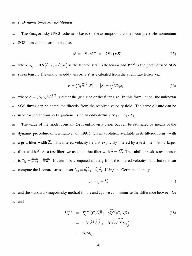
c. Dynamic Smagorinsky Method245

The Smagorinsky (1963) scheme is based on the assumption that the incompressible momentum246

SGS term can be parametrised as247

F =−∇ ·τττmod =−2∇ ·(νtSSS)

(15)

where Si j = 0.5(∂xiv j +∂x jvi

)is the filtered strain rate tensor and τττmod is the parametrised SGS248

stress tensor. The unknown eddy viscosity νt is evaluated from the strain rate tensor via249

νt =(CS∆

)2 ∣∣S∣∣ ;∣∣S∣∣=√2Si jSi j , (16)

where ∆ = (∆x∆y∆z)1/3 is either the grid size or the filter size. In this formulation, the unknown250

SGS fluxes can be computed directly from the resolved velocity field. The same closure can be251

used for scalar transport equations using an eddy diffusivity µt = νt/Prt.252

The value of the model constant CS is unknown a priori but can be estimated by means of the253

dynamic procedure of Germano et al. (1991). Given a solution available in its filtered form v with254

a grid filter width ∆. This filtered velocity field is explicitly filtered by a test filter with a larger255

filter width ∆. As a test filter, we use a top-hat filter with ∆ = 2∆. The subfilter-scale stress tensor256

is Ti j = uiu j− ui u j. It cannot be computed directly from the filtered velocity field, but one can257

compute the Leonard stress tensor Li j = ui u j− ui u j. Using the Germano identity258

Ti j = Li j + τi j (17)

and the standard Smagorinsky method for τi j and Tji, we can minimise the difference between Li j259

and260

Lmodi j = T mod

i j (C, ∆,vvv)− τmodi j (C,∆,vvv) (18)

= −2C∆2|S|Si j +2C

(∆

2|S|Si j

)= 2CMi j,

14

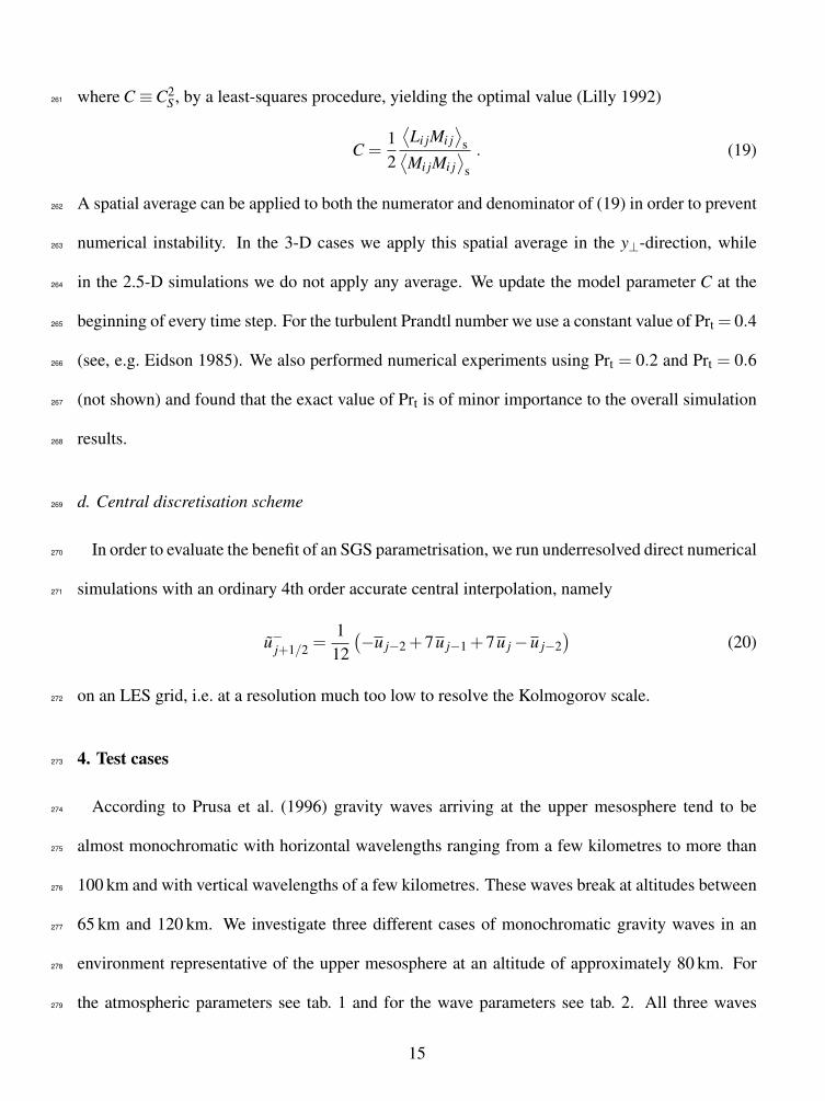
where C ≡C2S , by a least-squares procedure, yielding the optimal value (Lilly 1992)261

C =12

⟨Li jMi j

⟩s⟨

Mi jMi j⟩

s. (19)

A spatial average can be applied to both the numerator and denominator of (19) in order to prevent262

numerical instability. In the 3-D cases we apply this spatial average in the y⊥-direction, while263

in the 2.5-D simulations we do not apply any average. We update the model parameter C at the264

beginning of every time step. For the turbulent Prandtl number we use a constant value of Prt = 0.4265

(see, e.g. Eidson 1985). We also performed numerical experiments using Prt = 0.2 and Prt = 0.6266

(not shown) and found that the exact value of Prt is of minor importance to the overall simulation267

results.268

d. Central discretisation scheme269

In order to evaluate the benefit of an SGS parametrisation, we run underresolved direct numerical270

simulations with an ordinary 4th order accurate central interpolation, namely271

u−j+1/2 =1

12(−u j−2 +7u j−1 +7u j−u j−2

)(20)

on an LES grid, i.e. at a resolution much too low to resolve the Kolmogorov scale.272

4. Test cases273

According to Prusa et al. (1996) gravity waves arriving at the upper mesosphere tend to be274

almost monochromatic with horizontal wavelengths ranging from a few kilometres to more than275

100 km and with vertical wavelengths of a few kilometres. These waves break at altitudes between276

65 km and 120 km. We investigate three different cases of monochromatic gravity waves in an277

environment representative of the upper mesosphere at an altitude of approximately 80 km. For278

the atmospheric parameters see tab. 1 and for the wave parameters see tab. 2. All three waves279

15

have a wavelength of 3 km and the wave phase is such that, in the rotated coordinate system,280

the maximum total buoyancy gradient within the wave is located at ζ = 750m and the minimum281

(associated with the least stable point) at ζ = 2250m. The primary and secondary perturbations282

of the waves used to construct the initial condition for the 3-D simulations were computed by283

Fruman et al. (2014). In fig. 2 we show the initial perturbation energy Eini (primary and secondary284

perturbations) as a function of ζ , integrated in the spanwise–streamwise (x‖-y⊥) plane.285

Case 1 is a statically unstable inertia-gravity wave with a wave period of 8 hours and a phase286

speed of 0.1 m s−1. The wavelength of the leading transverse normal mode (primary perturbation)287

is somewhat longer than the base wavelength (λ‖= 3.98 km), while the leading secondary singular288

vector (with respect to an optimisation time of 5 minutes) has a significantly shorter wavelength289

(λ⊥= 0.4 km). The initial perturbation energy (fig. 2(a)) is distributed rather homogeneously in the290

wave with a peak close to the minimum static stability and a minimum in the most stable region.291

The time scales of the turbulent wave breaking and of the wave propagation are similarly long,292

which makes this case especially interesting. Remmler et al. (2013) pointed out that a secondary293

breaking event is stimulated in this cases when the most unstable part of the wave reaches the294

region where the primary breaking has earlier generated significant turbulence.295

Case 2 is also an inertia-gravity wave with the same period and phase speed as case 1, but with an296

amplitude below the threshold of static instability. The wave is perturbed by the leading transverse297

primary singular vector (λ‖ = 2.115 km), and the leading secondary singular vector (λ⊥ = 300 m).298

An optimisation time of 7.5 minutes was used for computing both the primary and secondary299

singular vectors. The perturbation energy in this case is concentrated exclusively in the region of300

lowest static stability (see fig. 2(b)). This is typical for SV, which maximise perturbation energy301

growth in a given time. Despite the wave being statically stable, the perturbations lead to a weak302

breaking and the generation of turbulence. However, the duration of the breaking event is much303

16

shorter than the wave period and the overall energy loss in the wave is not much larger than the304

energy loss through viscous forces on the base wave in the same time.305

Case 3 is a statically unstable high-frequency gravity wave with a period of 15 minutes and306

a phase speed of 3.3 m s−1 perturbed with the leading transverse primary normal mode (λ‖ =307

2.929 km) and the leading secondary singular vector with λ⊥ = 3 km. The initial perturbation308

energy (fig. 2(c)) has a clear maximum at ζ = 100m, which is in a region with moderately stable309

stratification. The breaking is much stronger than in cases 1 and 2 and lasts for slightly more310

than one wave period. Turbulence and energy dissipation are almost uniformly distributed in the311

domain during the most intense phase of the breaking.312

The three different cases were chosen to represent a wide range of different configurations of313

breaking gravity waves. They especially differ in the duration of the breaking compared to the314

wave period. In case 1 the breaking duration is slightly smaller than the wave period and the315

breaking involves multiple bursts of turbulence. In case 2 the breaking lasts only for a short time316

compared to the wave period and in case 3 the breaking lasts longer than one wave period.317

5. Case 1: unstable inertia-gravity wave318

a. Three-dimensional DNS319

Fruman et al. (2014) showed that in 2.5-D simulations a small initial random disturbance of the320

flow field can lead to different global results. In order to investigate whether the same applies321

to full 3-D simulations of the same case and whether the LES method has an influence on this322

variability, we added two new DNS simulations (640×64×500 cells) to the results of Remmler323

et al. (2013) to have a very small ensemble of four simulations from which we can compute324

averages and standard deviations. For these new simulations, a very small amount of white noise325

17

was added to all three velocity components at the initial time. In fig. 3 we show the ensemble326

average of the amplitudes 〈a〉e and of the spatially averaged total dissipation rate 〈εt〉s,e as a solid327

line and the standard deviation from these ensemble averages as shaded area.328

For the present case the wave breaking consists of a series of three single breaking events. Each329

of those events is characterised by a peak in the energy dissipation and by an enhanced amplitude330

decrease. The strongest breaking event is initialised by the initial perturbations and starts directly331

at the beginning of the simulation. It involves overturning and generation of turbulence in the332

whole computational domain. The intensity of this primary breaking event is very similar in all333

ensemble members, independent of the resolution and initial white noise. The second breaking334

event around t ≈ 4 h is preceeded by an instability of the large-scale wave and generates only a335

small amount of turbulence in the unstable half of the domain. The third breaking event around336

t ≈ 5 h is caused by a small amount of remaining turbulence from the first breaking event, which337

was generated in the stable part of the wave. At the time of the third breaking event the wave phase338

has travelled approximately half a wavelength and so the unstable part of the wave has reached the339

region of the remaining turbulence at this time. For details of the wave breaking process, we refer340

to Remmler et al. (2013) and Fruman et al. (2014).341

The amplitude variations in the 3-D DNS are very small. The ensemble members diverge slightly342

during a very weak breaking event at t ≈ 8 h, which has very different intensity in the four simula-343

tions. The total dissipation rate varies significantly among the ensemble members during the weak344

breaking events but not during the first strong breaking event.345

b. Three-dimensional LES346

We simulated the 3-D setup of case 1 using three different LES resolutions, which we refer to347

as fine (100× 24× 80 cells, corresponding to a cell size of 39.8m× 17.7m× 37.5m), medium348

18

(24× 12× 80 cells) and coarse (24× 12× 20 cells). We chose these resolutions after a series of349

numerical experiments which showed two main results: (i) the horizontal (i.e. in the x‖-y⊥ plane)350

resolution can be reduced without much effect on the global result as long as the vertical resolution351

remains comparatively high, and (ii) reducing the vertical resolution and keeping the horizontal352

resolution high had a strong adverse effect on the global result, independent of the LES method353

used. One reason for this behaviour might be the insufficient resolution of the initial perturbation354

on the coarsest grid. From fig. 2(a) it is obvious that the initial perturbation is well resolved by355

80 cells in the ζ direction, but deviates in places on the coarse grid with only 20 cells in the ζ356

direction.357

In LES it is easily affordable to run small ensembles for many different simulations. For all358

presented 3-D LES results we performed the same simulation eight times with some low-level359

white noise superposed on the initial condition (consisting of the base wave and its leading primary360

and secondary perturbations) and once with no added noise. The results of these nine realisations361

were then averaged. The average amplitudes of simulations with three different resolutions and362

four different LES methods (standard ALDM with β = 0.0, modified ALDM with β = 0.01,363

Dynamic Smagorinsky [DSM], and plain central discretisation [CDS4]) are shown in figs. 3(a) to364

3(c). Figure 3(d) shows the total dissipation rates for the medium grid. In all figures the error bars365

indicate the standard deviation of the ensemble.366

Using the fine LES grid the average wave amplitude is quite well predicted by standard ALDM,367

DSM and CDS4. Modified ALDM dissipates slightly too much energy while standard ALDM368

shows very large variations between ensemble members.369

With the medium grid the three SGS models (i.e. DSM and the two versions of ALDM) yield370

good agreement with the DNS, both in the average amplitude and in the variations among ensemble371

members. Only CDS4 (without SGS model) creates a bit too much dissipation and far too much372

19

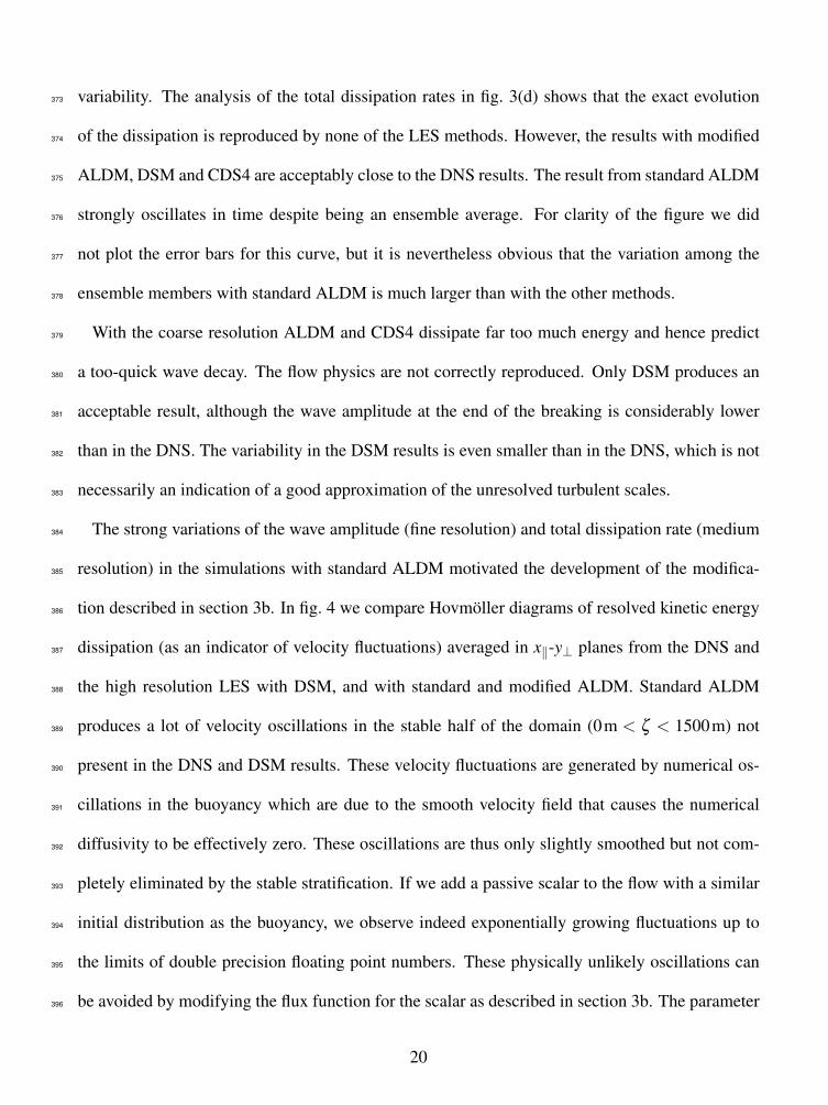
variability. The analysis of the total dissipation rates in fig. 3(d) shows that the exact evolution373

of the dissipation is reproduced by none of the LES methods. However, the results with modified374

ALDM, DSM and CDS4 are acceptably close to the DNS results. The result from standard ALDM375

strongly oscillates in time despite being an ensemble average. For clarity of the figure we did376

not plot the error bars for this curve, but it is nevertheless obvious that the variation among the377

ensemble members with standard ALDM is much larger than with the other methods.378

With the coarse resolution ALDM and CDS4 dissipate far too much energy and hence predict379

a too-quick wave decay. The flow physics are not correctly reproduced. Only DSM produces an380

acceptable result, although the wave amplitude at the end of the breaking is considerably lower381

than in the DNS. The variability in the DSM results is even smaller than in the DNS, which is not382

necessarily an indication of a good approximation of the unresolved turbulent scales.383

The strong variations of the wave amplitude (fine resolution) and total dissipation rate (medium384

resolution) in the simulations with standard ALDM motivated the development of the modifica-385

tion described in section 3b. In fig. 4 we compare Hovmoller diagrams of resolved kinetic energy386

dissipation (as an indicator of velocity fluctuations) averaged in x‖-y⊥ planes from the DNS and387

the high resolution LES with DSM, and with standard and modified ALDM. Standard ALDM388

produces a lot of velocity oscillations in the stable half of the domain (0m < ζ < 1500m) not389

present in the DNS and DSM results. These velocity fluctuations are generated by numerical os-390

cillations in the buoyancy which are due to the smooth velocity field that causes the numerical391

diffusivity to be effectively zero. These oscillations are thus only slightly smoothed but not com-392

pletely eliminated by the stable stratification. If we add a passive scalar to the flow with a similar393

initial distribution as the buoyancy, we observe indeed exponentially growing fluctuations up to394

the limits of double precision floating point numbers. These physically unlikely oscillations can395

be avoided by modifying the flux function for the scalar as described in section 3b. The parameter396

20

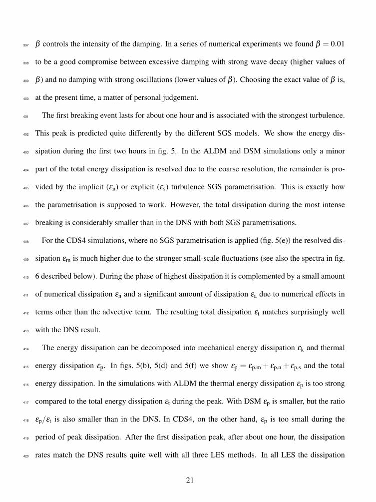
β controls the intensity of the damping. In a series of numerical experiments we found β = 0.01397

to be a good compromise between excessive damping with strong wave decay (higher values of398

β ) and no damping with strong oscillations (lower values of β ). Choosing the exact value of β is,399

at the present time, a matter of personal judgement.400

The first breaking event lasts for about one hour and is associated with the strongest turbulence.401

This peak is predicted quite differently by the different SGS models. We show the energy dis-402

sipation during the first two hours in fig. 5. In the ALDM and DSM simulations only a minor403

part of the total energy dissipation is resolved due to the coarse resolution, the remainder is pro-404

vided by the implicit (εn) or explicit (εs) turbulence SGS parametrisation. This is exactly how405

the parametrisation is supposed to work. However, the total dissipation during the most intense406

breaking is considerably smaller than in the DNS with both SGS parametrisations.407

For the CDS4 simulations, where no SGS parametrisation is applied (fig. 5(e)) the resolved dis-408

sipation εm is much higher due to the stronger small-scale fluctuations (see also the spectra in fig.409

6 described below). During the phase of highest dissipation it is complemented by a small amount410

of numerical dissipation εn and a significant amount of dissipation εa due to numerical effects in411

terms other than the advective term. The resulting total dissipation εt matches surprisingly well412

with the DNS result.413

The energy dissipation can be decomposed into mechanical energy dissipation εk and thermal414

energy dissipation εp. In figs. 5(b), 5(d) and 5(f) we show εp = εp,m + εp,n + εp,s and the total415

energy dissipation. In the simulations with ALDM the thermal energy dissipation εp is too strong416

compared to the total energy dissipation εt during the peak. With DSM εp is smaller, but the ratio417

εp/εt is also smaller than in the DNS. In CDS4, on the other hand, εp is too small during the418

period of peak dissipation. After the first dissipation peak, after about one hour, the dissipation419

rates match the DNS results quite well with all three LES methods. In all LES the dissipation420

21

peaks a little bit earlier than in the DNS. The time difference is surely due to the time that flow421

energy needs to be transported through the spectrum from the finest LES scales to the scales of422

maximum dissipation in the DNS.423

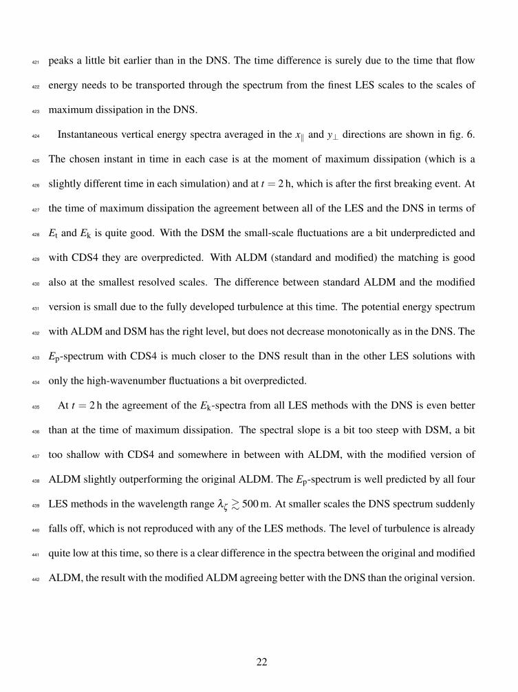
Instantaneous vertical energy spectra averaged in the x‖ and y⊥ directions are shown in fig. 6.424

The chosen instant in time in each case is at the moment of maximum dissipation (which is a425

slightly different time in each simulation) and at t = 2 h, which is after the first breaking event. At426

the time of maximum dissipation the agreement between all of the LES and the DNS in terms of427

Et and Ek is quite good. With the DSM the small-scale fluctuations are a bit underpredicted and428

with CDS4 they are overpredicted. With ALDM (standard and modified) the matching is good429

also at the smallest resolved scales. The difference between standard ALDM and the modified430

version is small due to the fully developed turbulence at this time. The potential energy spectrum431

with ALDM and DSM has the right level, but does not decrease monotonically as in the DNS. The432

Ep-spectrum with CDS4 is much closer to the DNS result than in the other LES solutions with433

only the high-wavenumber fluctuations a bit overpredicted.434

At t = 2 h the agreement of the Ek-spectra from all LES methods with the DNS is even better435

than at the time of maximum dissipation. The spectral slope is a bit too steep with DSM, a bit436

too shallow with CDS4 and somewhere in between with ALDM, with the modified version of437

ALDM slightly outperforming the original ALDM. The Ep-spectrum is well predicted by all four438

LES methods in the wavelength range λζ & 500 m. At smaller scales the DNS spectrum suddenly439

falls off, which is not reproduced with any of the LES methods. The level of turbulence is already440

quite low at this time, so there is a clear difference in the spectra between the original and modified441

ALDM, the result with the modified ALDM agreeing better with the DNS than the original version.442

22

c. 2.5-D simulations443

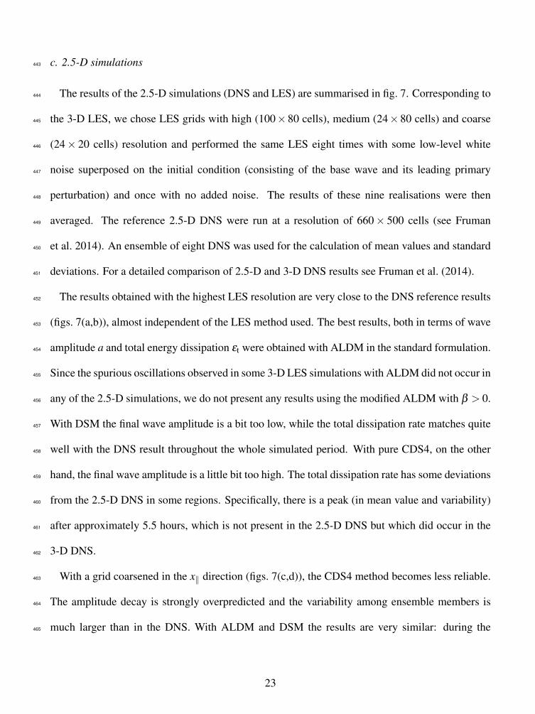
The results of the 2.5-D simulations (DNS and LES) are summarised in fig. 7. Corresponding to444

the 3-D LES, we chose LES grids with high (100×80 cells), medium (24×80 cells) and coarse445

(24× 20 cells) resolution and performed the same LES eight times with some low-level white446

noise superposed on the initial condition (consisting of the base wave and its leading primary447

perturbation) and once with no added noise. The results of these nine realisations were then448

averaged. The reference 2.5-D DNS were run at a resolution of 660× 500 cells (see Fruman449

et al. 2014). An ensemble of eight DNS was used for the calculation of mean values and standard450

deviations. For a detailed comparison of 2.5-D and 3-D DNS results see Fruman et al. (2014).451

The results obtained with the highest LES resolution are very close to the DNS reference results452

(figs. 7(a,b)), almost independent of the LES method used. The best results, both in terms of wave453

amplitude a and total energy dissipation εt were obtained with ALDM in the standard formulation.454

Since the spurious oscillations observed in some 3-D LES simulations with ALDM did not occur in455

any of the 2.5-D simulations, we do not present any results using the modified ALDM with β > 0.456

With DSM the final wave amplitude is a bit too low, while the total dissipation rate matches quite457

well with the DNS result throughout the whole simulated period. With pure CDS4, on the other458

hand, the final wave amplitude is a little bit too high. The total dissipation rate has some deviations459

from the 2.5-D DNS in some regions. Specifically, there is a peak (in mean value and variability)460

after approximately 5.5 hours, which is not present in the 2.5-D DNS but which did occur in the461

3-D DNS.462

With a grid coarsened in the x‖ direction (figs. 7(c,d)), the CDS4 method becomes less reliable.463

The amplitude decay is strongly overpredicted and the variability among ensemble members is464

much larger than in the DNS. With ALDM and DSM the results are very similar: during the465

23

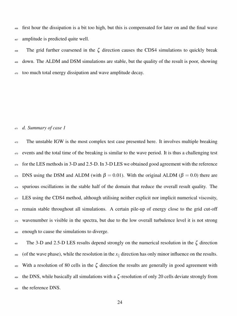
first hour the dissipation is a bit too high, but this is compensated for later on and the final wave466

amplitude is predicted quite well.467

The grid further coarsened in the ζ direction causes the CDS4 simulations to quickly break468

down. The ALDM and DSM simulations are stable, but the quality of the result is poor, showing469

too much total energy dissipation and wave amplitude decay.470

d. Summary of case 1471

The unstable IGW is the most complex test case presented here. It involves multiple breaking472

events and the total time of the breaking is similar to the wave period. It is thus a challenging test473

for the LES methods in 3-D and 2.5-D. In 3-D LES we obtained good agreement with the reference474

DNS using the DSM and ALDM (with β = 0.01). With the original ALDM (β = 0.0) there are475

spurious oscillations in the stable half of the domain that reduce the overall result quality. The476

LES using the CDS4 method, although utilising neither explicit nor implicit numerical viscosity,477

remain stable throughout all simulations. A certain pile-up of energy close to the grid cut-off478

wavenumber is visible in the spectra, but due to the low overall turbulence level it is not strong479

enough to cause the simulations to diverge.480

The 3-D and 2.5-D LES results depend strongly on the numerical resolution in the ζ direction481

(of the wave phase), while the resolution in the x‖ direction has only minor influence on the results.482

With a resolution of 80 cells in the ζ direction the results are generally in good agreement with483

the DNS, while basically all simulations with a ζ -resolution of only 20 cells deviate strongly from484

the reference DNS.485

24

6. Case 2: Stable inertia-gravity wave486


The reference DNS results are taken from Fruman et al. (2014). They presented simulations488

with 720× 96× 1024 cells and with 512× 64× 768 cells. To have at least a small ensemble of489

four members for comparison, we repeated these simulations (adding low level white noise to the490

velocity components of the initial condition) running until t = 1 h. The ensemble average and491

standard deviation of these four simulations is shown in fig. 8.492

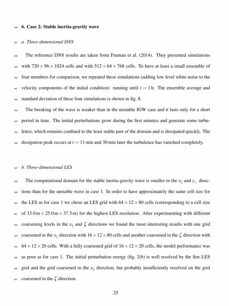
The breaking of the wave is weaker than in the unstable IGW case and it lasts only for a short493

period in time. The initial perturbations grow during the first minutes and generate some turbu-494

lence, which remains confined to the least stable part of the domain and is dissipated quickly. The495

dissipation peak occurs at t = 11 min and 30 min later the turbulence has vanished completely.496


The computational domain for the stable inertia-gravity wave is smaller in the x‖ and y⊥ direc-498

tions than for the unstable wave in case 1. In order to have approximately the same cell size for499

the LES as for case 1 we chose an LES grid with 64×12×80 cells (corresponding to a cell size500

of 33.0m× 25.0m× 37.5m) for the highest LES resolution. After experimenting with different501

coarsening levels in the x‖ and ζ directions we found the most interesting results with one grid502

coarsened in the x‖ direction with 16×12×80 cells and another coarsened in the ζ direction with503

64×12×20 cells. With a fully coarsened grid of 16×12×20 cells, the model performance was504

as poor as for case 1. The initial perturbation energy (fig. 2(b) is well resolved by the fine LES505

grid and the grid coarsened in the x‖ direction, but probably insufficiently resolved on the grid506

coarsened in the ζ direction.507

25

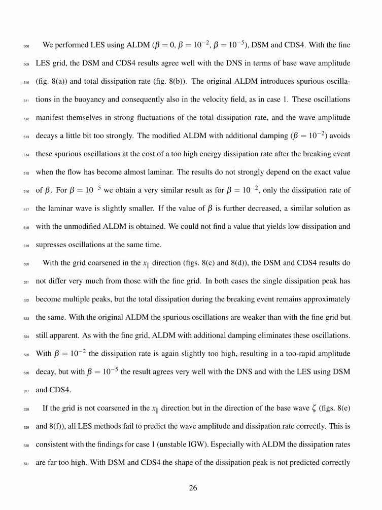
We performed LES using ALDM (β = 0, β = 10−2, β = 10−5), DSM and CDS4. With the fine508

LES grid, the DSM and CDS4 results agree well with the DNS in terms of base wave amplitude509

(fig. 8(a)) and total dissipation rate (fig. 8(b)). The original ALDM introduces spurious oscilla-510

tions in the buoyancy and consequently also in the velocity field, as in case 1. These oscillations511

manifest themselves in strong fluctuations of the total dissipation rate, and the wave amplitude512

decays a little bit too strongly. The modified ALDM with additional damping (β = 10−2) avoids513

these spurious oscillations at the cost of a too high energy dissipation rate after the breaking event514

when the flow has become almost laminar. The results do not strongly depend on the exact value515

of β . For β = 10−5 we obtain a very similar result as for β = 10−2, only the dissipation rate of516

the laminar wave is slightly smaller. If the value of β is further decreased, a similar solution as517

with the unmodified ALDM is obtained. We could not find a value that yields low dissipation and518

supresses oscillations at the same time.519

With the grid coarsened in the x‖ direction (figs. 8(c) and 8(d)), the DSM and CDS4 results do520

not differ very much from those with the fine grid. In both cases the single dissipation peak has521

become multiple peaks, but the total dissipation during the breaking event remains approximately522

the same. With the original ALDM the spurious oscillations are weaker than with the fine grid but523

still apparent. As with the fine grid, ALDM with additional damping eliminates these oscillations.524

With β = 10−2 the dissipation rate is again slightly too high, resulting in a too-rapid amplitude525

decay, but with β = 10−5 the result agrees very well with the DNS and with the LES using DSM526

and CDS4.527

If the grid is not coarsened in the x‖ direction but in the direction of the base wave ζ (figs. 8(e)528

and 8(f)), all LES methods fail to predict the wave amplitude and dissipation rate correctly. This is529

consistent with the findings for case 1 (unstable IGW). Especially with ALDM the dissipation rates530

are far too high. With DSM and CDS4 the shape of the dissipation peak is not predicted correctly531

26

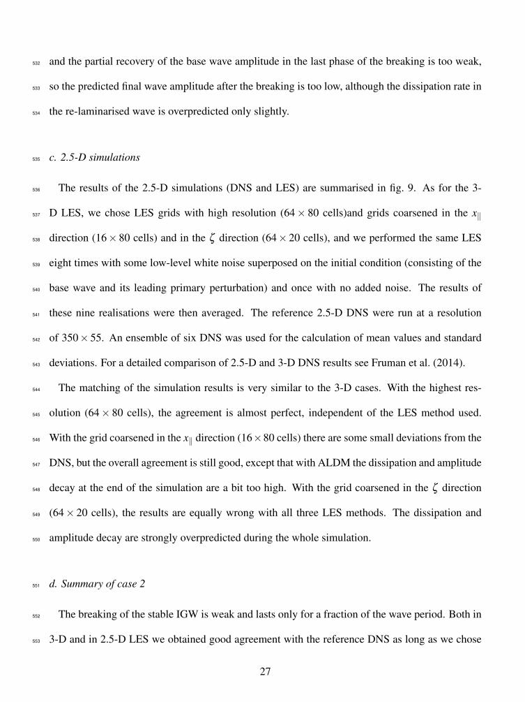
and the partial recovery of the base wave amplitude in the last phase of the breaking is too weak,532

so the predicted final wave amplitude after the breaking is too low, although the dissipation rate in533

the re-laminarised wave is overpredicted only slightly.534


The results of the 2.5-D simulations (DNS and LES) are summarised in fig. 9. As for the 3-536

D LES, we chose LES grids with high resolution (64× 80 cells)and grids coarsened in the x‖537

direction (16× 80 cells) and in the ζ direction (64× 20 cells), and we performed the same LES538

eight times with some low-level white noise superposed on the initial condition (consisting of the539

base wave and its leading primary perturbation) and once with no added noise. The results of540

these nine realisations were then averaged. The reference 2.5-D DNS were run at a resolution541

of 350× 55. An ensemble of six DNS was used for the calculation of mean values and standard542

deviations. For a detailed comparison of 2.5-D and 3-D DNS results see Fruman et al. (2014).543

The matching of the simulation results is very similar to the 3-D cases. With the highest res-544

olution (64× 80 cells), the agreement is almost perfect, independent of the LES method used.545

With the grid coarsened in the x‖ direction (16×80 cells) there are some small deviations from the546

DNS, but the overall agreement is still good, except that with ALDM the dissipation and amplitude547

decay at the end of the simulation are a bit too high. With the grid coarsened in the ζ direction548

(64× 20 cells), the results are equally wrong with all three LES methods. The dissipation and549

amplitude decay are strongly overpredicted during the whole simulation.550


The breaking of the stable IGW is weak and lasts only for a fraction of the wave period. Both in552

3-D and in 2.5-D LES we obtained good agreement with the reference DNS as long as we chose553

27

a comparatively high resolution in the ζ direction, while the results were not much affected by554

choosing a low resolution in the x‖ direction. Since the 2.5-D DNS were sufficient for estimating555

the breaking duration and intensity, see Fruman et al. (2014), LES with only 16×80 = 1280 cells556

are thus sufficient for computing the basic characteristic of the wave breaking. Good LES results557

were obtained without any SGS parametrisation and with DSM.558

7. Case 3: Unstable high-frequency gravity wave559


Fruman et al. (2014) simulated the case of a breaking unstable HGW on grids with 15363 cells,561

7683 cells and 3843 cells. They found no notable differences between the two highest resolutions.562

We added another two simulations with 7683 cells and 3843 cells and averaged the results of these563

five DNS. The results are presented in fig. 10.564

The wave breaking is much more intense than in both IGW cases. The generation of turbulence565

starts immediately after the initialisation in the unstable part of the wave and is quickly advected566

also into the stable part due to the high phase velocity of the wave. At the time of maximum567

energy dissipation (around t = 15 min) turbulence is distributed almost homogeneously in the568

whole domain. The non-dimensional wave amplitude rapidly decreases from an initial value of569

a = 1.2 to a ≈ 0.3 after 30 min and does not change significantly any more after that time. The570

breaking process is analysed in more detail by Fruman et al. (2014).571


The domain for the unstable high-frequency gravity wave case is almost cubic. In a number573

of LES with different resolutions in the horizontal and the vertical directions we could not find574

any indication that different resolutions in the different directions make a great deal of difference.575

28

Hence we present here the results of three LES grids with coarse (203), medium (403) and fine576

(803), the fine resolution corresponding to a cell size of 36.6m×37.5m×37.5m) resolution. On577

the medium and fine grid, the initial perturbation is resolved almost perfectly (see fig. 2(c)), while578

on the coarse grid there are some slight deviations in the initial perturbation energy distribution.579

We performed LES on these grids using ALDM (β = 0, β = 0.01), DSM and CDS4. For all of580

these cases we averaged the results of nine simulations to get an estimate of the ensemble average581

and the standard deviations.582

With the high LES resolution of 803 cells, the results are very similar to the DNS (figs. 10(a)583

and 10(b)). The base wave amplitude decay is slightly overpredicted with ALDM and CDS4, but584

the amplitude remains almost within the variations among the DNS ensemble members. The peak585

dissipation rate matches well with the DNS in all cases. With CDS4 the dissipation falls off a bit586

too rapidly after the peak. With modified ALDM (β = 0.01) the dissipation rate is overpredicted587

during the phases of weak turbulence, i.e. before and after the peak. Actually, using the modified588

version is not necessary for this simulation, since no physically unlikely oscillations develop at589

any time due to the high level of turbulence during most of the simulation.590

When the resolution is reduced to 403 cells (figs. 10(c) and 10(d)) the main difference is in the591

CDS4 simulations. The turbulence during the peak of breaking is too strong and the molecular592

dissipation is not sufficient on the coarse grid to keep the energy balance. Energy piles up at593

the smallest resolved wavenumbers (see the energy spectra in fig. 12) and numerical errors lead594

to an increase of flow total energy, which eventually also affects the largest resolved scales, and595

therefore the amplitude of the base wave. The time of simulation break-down is almost the same596

in all ensemble members. By using the turbulence parametrisation schemes this instability can be597

avoided. The best matching with the DNS results is obtained with the original ALDM. Only about598

10% of the peak energy dissipation is resolved, see fig. 11(a), but the sum of resolved molecular599

29

and numerical dissipation matches quite well with the DNS result. Also the ratio between εk and600

εp is well repoduced, see fig. 11(b). The modified ALDM dissipates too much energy. The DSM601

predicts a slightly too-high base wave amplitude after the breaking and the total dissipation rate602

starts oscillating moderately after approximately 60 min. The total dissipation rate presented in603

fig. 11(c) is overpredicted a bit at the peak, but matches well with the DNS before t = 10 min and604

after t = 15 min.605

In fig. 12 we present the energy spectra of all LES with 403 cells compared to the DNS spectra.606

The CDS4 spectra are wrong, as mentioned above, and the method fails for this case. The ALDM607

and DSM spectra are very close to the DNS reference for wavelengths λζ > 400 m. For smaller608

wavelengths the spectral energy is slightly underpredicted with only very small differences be-609

tween ALDM (β = 0.0) and DSM. With ALDM (β = 0.01), the thermal energy dissipation εp is610

overpredicted, hence the spectra of potential and total energy fall off to rapidly close to the grid611

cut-off wavelength.612

The results obtained with the coarsest grid, with 203 cells (figs. 10(e) and 10(f)), are similar613

to those with the medium resolution. The simulations with CDS4 break down due to unbounded614

growth of numerical errors. ALDM with β = 0.01 is far too dissipative before and after the peak615

of dissipation. The DSM now underpredicts the final wave amplitude and generates oscillations of616

total dissipation after the breaking. The closest match with the DNS is obtained with the original617

ALDM, both in terms of base wave amplitude and total dissipation rate. Also the variations among618

ensemble members are similar to the DNS. The onset of dissipation is, in all LES a little bit earlier619

than in the DNS. This is consistent with our observations in case 1.620

30


The results of the 2.5-D simulations (DNS and LES) are summarised in figure 13. LES grids with622

high (802 cells), medium (402 cells) and coarse resolution (202 cells) were used. The same LES623

were performed eight times with some low-level white noise superposed on the initial condition624

(consisting of the base wave and its leading primary perturbation) and once with no added noise.625

The results of these nine realisations were then averaged. The reference 2.5-D DNS were run at626

a resolution of 500× 500 cells. An ensemble of six DNS was used for the calculation of mean627

values and standard deviations.628

With the highest resolution (802 cells), the results in terms of wave amplitude and total dissi-629

pation rate are in very close agreement with the reference DNS. Only for CDS4 is the dissipation630

rate a bit too low during the period of decreasing dissipation.631

At the medium resolution (402 cells), the DSM and ALDM results are very similar and still in632

good agreement with the DNS. The dissipation peak is slightly shifted to earlier times according to633

the dissipation acting at larger wavenumbers and the hence reduced time required for flow energy634

to reach this range. CDS4, however, predicts the wrong evolution of the wave amplitude and635

dissipation rate and cannot be recommended for this resolution.636

At the coarsest resolution (202 cells), ALDM and DSM still do a very good job in predicting the637

amplitude decay and the dissipation maximum. The dissipation peak is further shifted forward in638

time due to the reduced time the flow energy needs to move through the spectrum. In the CDS4639

simulation, however, the dissipation rate becomes negative after approximately 20 minutes and640

hence the predicted flow field is completely wrong, although the simulations remain stable in a641

numerical sense during the whole simulated period.642

31


The unstable HGW involves much stronger turbulence than the IGW cases and thus the buoy-644

ancy forces are weaker compared to the acceleration associated with turbulent motions. The orig-645

inal ALDM and the DSM thus do an excellent job in predicting the dissipation rates and the wave646

amplitude decay over time, even at a very coarse resolution with a cell size of about ∆ = 150 m,647

both in 3-D and 2.5-D simulations. According to Fruman et al. (2014) the 3-D and the 2.5-D648

solutions are similar in this case. We conclude that for a proper estimation of the key parameters649

breaking time, maximum dissipation and amplitude decay only a 2.5-D simulation with 202 = 400650

cells is necessary, if ALDM or DSM is applied.651

8. Conclusion652

We scrutinised different methods of large-eddy simulation for three cases of breaking monochro-653

matic gravity waves. The methods tested included: the Adaptive Local Deconvolution Method654

(ALDM), an implicit turbulence parametrisation; the dynamic Smagorinsky method (DSM); and a655

plain fourth order central discretisation without any turbulence parametrisation (CDS4). The test656

cases have been carefully designed and set-up by Remmler et al. (2013) and Fruman et al. (2014)657

based on the primary and secondary instability modes of the base waves and included an unstable658

and a stable inertia-gravity wave as well as an unstable high-frequency gravity wave. All simu-659

lations presented were run in 2.5-D and 3-D domains and for all simulations a small ensemble of660

simulations starting from slightly different initial conditions were performed in order to assess the661

sensitivity and robustness of the results.662

The original ALDM leads to spurious oscillations of the buoyancy field in some 3-D simulations,663

where the velocity field is very smooth for a long time. We thus developed a modified version of664

32

the ALDM flux function. The modification led to a significant reduction of the oscillations, but665

also increased the overall energy dissipation.666

For all three test cases we started at an LES resolution of 80 cells per wavelength of the original667

wave and gradually reduced the resolution in all three directions. The inertia-gravity wave cases,668

in which the wave vector almost coincides with the vertical direction, were very sensitive to the669

resolution in the direction of the wave vector, while the resolution in the other directions could be670

strongly reduced without a massive negative effect on the overall results.671

We found that results obtained with ALDM and DSM are generally in good agreement with672

the reference direct numerical simulations as long as the resolution in the direction of the wave673

vector is sufficiently high. The CDS4 simulations, without turbulence parametrisation, are only674

successful if the resolution is high and the level of turbulence comparatively low. In cases with675

low turbulence intensity and a smooth velocity field for long time periods (unstable and stable676

IGW) ALDM generated spurious oscillations in the buoyancy field, which we could avoid by677

using the modified numerical flux function. However, this was not necessary in the case with a678

high turbulence level (unstable HGW) and in all 2.5-D simulations.679

Our results back the findings of Remmler and Hickel (2012, 2013, 2014), who showed that both680

DSM and ALDM are suitable tools for the simulation of homogeneous stratified turbulence. Ap-681

plying the same methods to gravity-wave breaking, where turbulence is spatially inhomogeneous682

and intermittent in time, reveals that DSM is in some cases more robust than ALDM, although683

ALDM provides a better approximation of the spectral eddy viscosity and diffusivity in homoge-684

neous stratified turbulence (Remmler and Hickel 2014).685

In all simulations we observed that the peak of dissipation occurs earlier in simulations with686

coarser computational grids. This is more pronounced in 2.5-D LES, but also apparent in 3-687

D LES. We explain this time difference by the time required for flow energy to move from the688

33

smallest resolved wavenumbers in an LES to the dissipative scales in a DNS. Among the tested689

LES methods there is no method that can account for this time lag. However, the large-scale flow690

and the maximum dissipation can still be predicted correctly.691

Fruman et al. (2014) have shown that in some cases 2.5-D simulations can be sufficient to get a692

good estimate of the energy dissipation during a breaking event. We showed that with ALDM and693

DSM reliable results can be obtained in 2.5-D simulations with less than 2000 computational cells.694

Such inexpensive simulations will allow running large numbers of simulations in order to study695

the influence of various parameters on wave breaking, such as stratification, wavelength, ampli-696

tude, propagation angle and viscosity. A possible automated approach would involve computing697

the growth rates of perturbations of the original waves, setting up an ensemble of 2.5-D LES ini-698

tialised by the base wave and its leading primary perturbation and extracting key data from the699

LES results, such as the maximum energy dissipation, the amplitude decay and the duration of the700

breaking event. Another potential application of our findings is the (2.5-D or 3-D) simulation of701

wave packets in the atmosphere, which is computationally feasible only if small-scale turbulence702

remains unresolved and is treated by a reliable subgrid-scale parametrisation such as ALDM or703

DSM.704

Acknowledgment. U. A. and S. H. thank Deutsche Forschungsgemeinschaft for partial support705

through the MetStrom (Multiple Scales in Fluid Mechanics and Meteorology) Priority Research706

Program (SPP 1276), and through Grants HI 1273/1-2 and AC 71/4-2. Computational resources707

were provided by the HLRS Stuttgart under the grant DINSGRAW.708

References709

Achatz, U., 2005: On the role of optimal perturbations in the instability of monochromatic gravity710

waves. Phys. Fluids, 17 (9), 094107.711

34

Achatz, U. and G. Schmitz, 2006a: Optimal growth in inertia-gravity wave packets: Energetics,712

long-term development, and three-dimensional structure. J. Atmos. Sci., 63, 414–434.713

Achatz, U. and G. Schmitz, 2006b: Shear and static instability of inertia-gravity wave packets:714

Short-term modal and nonmodal growth. J. Atmos. Sci., 63, 397–413.715

Afanasyev, Y. D. and W. R. Peltier, 2001: Numerical simulations of internal gravity wave breaking716

in the middle atmosphere: The influence of dispersion and three-dimensionalization. J. Atmos.717

Sci., 58, 132–153.718

Andreassen, Ø., P. Øyvind Hvidsten, D. C. Fritts, and S. Arendt, 1998: Vorticity dynamics in a719

breaking internal gravity wave. Part 1. Initial instability evolution. J. Fluid Mech., 367, 27–46.720

Baldwin, M. P., et al., 2001: The quasi-biennial oscillation. Rev. Geophys., 39, 179–229.721

Chun, H.-Y., M.-D. Song, J.-W. Kim, and J.-J. Baik, 2001: Effects of gravity wave drag induced722

by cumulus convection on the atmospheric general circulation. J. Atmos. Sci., 58 (3), 302–319.723

Dornbrack, A., 1998: Turbulent mixing by breaking gravity waves. J. Fluid Mech., 375, 113–141.724

Dunkerton, T. J., 1997: Shear instability of internal inertia-gravity waves. J. Atmos. Sci., 54, 1628–725

1641.726

Eidson, T. M., 1985: Numerical simulation of the turbulent Rayleigh–Benard problem using sub-727

grid modelling. J. Fluid Mech., 158, 245–268.728

Fritts, D. C. and M. J. Alexander, 2003: Gravity wave dynamics and effects in the middle atmo-729

sphere. Rev. Geophys., 41 (1).730

Fritts, D. C. and L. Wang, 2013: Gravity wave-fine structure interactions. Part II: Energy dissipa-731

tion evolutions, statistics, and implications. J. Atmos. Sci., 70 (12), 3710–3734.732

35

Fritts, D. C., L. Wang, J. Werne, T. Lund, and K. Wan, 2009: Gravity wave instability dynamics at733

high reynolds numbers. Parts I and II. J. Atmos. Sci., 66 (5), 1126–1171.734

Fritts, D. C., L. Wang, and J. A. Werne, 2013: Gravity wave-fine structure interactions. Part I:735

Influences of fine structure form and orientation on flow evolution and instability. J. Atmos. Sci.,736

70 (12), 3710–3734.737

Fruman, M. D. and U. Achatz, 2012: Secondary instabilities in breaking inertia-gravity waves. J.738

Atmos. Sci., 69, 303–322.739

Fruman, M. D., S. Remmler, U. Achatz, and S. Hickel, 2014: On the construction of a direct740

numerical simulation of a breaking inertia-gravity wave in the upper-mesosphere. J. Geophys.741

Res., 119, 11 613–11 640.742

Germano, M., U. Piomelli, P. Moin, and W. H. Cabot, 1991: A dynamic subgrid-scale eddy vis-743

cosity model. Phys. Fluids A, 3 (7), 1760–1765.744

Grimsdell, A. W., M. J. Alexander, P. T. May, and L. Hoffmann, 2010: Model study of waves745

generated by convection with direct validation via satellite. J. Atmos. Sci., 67 (5), 1617–1631.746

Hickel, S. and N. A. Adams, 2007: A proposed simplification of the adaptive local deconvolution747

method. ESAIM, 16, 66–76.748

Hickel, S., N. A. Adams, and J. A. Domaradzki, 2006: An adaptive local deconvolution method749

for implicit LES. J. Comput. Phys., 213, 413–436.750

Hickel, S., N. A. Adams, and N. N. Mansour, 2007: Implicit subgrid-scale modeling for large-eddy751

simulation of passive scalar mixing. Phys. Fluids, 19, 095 102.752

36

Hickel, S., C. Egerer, and J. Larsson, 2014: Subgrid-scale modeling for implicit large eddy sim-753

ulation of compressible flows and shock-turbulence interaction. Phys. Fluids, 26, 106 101, doi:754

10.1063/1.4898641.755

Hickel, S., T. Kempe, and N. A. Adams, 2008: Implicit large-eddy simulation applied to turbulent756

channel flow with periodic constrictions. Theor. Comput. Fluid Dyn., 22, 227–242.757

Hines, C. O., 1965: Dynamical heating of the upper atmosphere. J. Geophys. Res., 70 (1), 177–758

183.759

Hines, C. O., 1997: Doppler-spread parameterization of gravity-wave momentum deposition in760

the middle atmosphere. Part 1: Basic formulation. J. Atmos. Sol.-Terr. Phys., 59 (4), 371–386.761

Kim, Y.-J., S. D. Eckermann, and H.-Y. Chun, 2003: An overview of the past, present and future762

of gravity–wave drag parametrization for numerical climate and weather prediction models.763

Atmosphere-Ocean, 41 (1), 65–98.764

Lelong, M.-P. and T. J. Dunkerton, 1998: Inertia-gravity wave breaking in three dimensions. Parts765

I and II. J. Atmos. Sci., 55, 2473–2501.766

Lilly, D. K., 1992: A proposed modification of the german subgrid-scale closure method. Phys.767

Fluids A, 4 (3), 633–635.768

Lindzen, R. S., 1981: Turbulence and stress owing to gravity wave and tidal breakdown. J. Geo-769

phys. Res., 86, 9707–9714.770

Lund, T. S. and D. C. Fritts, 2012: Numerical simulation of gravity wave breaking in the lower771

thermosphere. J. Geophys. Res., 117 (D21105).772

McFarlane, N. A., 1987: The effect of orographically excited gravity wave drag on the general773

circulation of the lower stratosphere and troposphere. J. Atmos. Sci., 44, 1775–1800.774

37

McLandress, C., 1998: On the importance of gravity waves in the middle atmosphere and their775

parameterization in general circulation models. J. Atmos. Sol.-Terr. Phy., 60 (14), 1357–1383.776

Muraschko, J., M. D. Fruman, U. Achatz, S. Hickel, and Y. Toledo, 2014: On the application777

of Wentzel–Kramer–Brillouin theory for the simulation of the weakly nonlinear dynamics of778

gravity waves. Q. J. R. Meteorol. Soc., doi:10.1002/qj.2381.779

O’Sullivan, D. and T. J. Dunkerton, 1995: Generation of inertia-gravity waves in a simulated life780

cycle of baroclinic instability. J. Atmos. Sci., 52 (21), 3695–3716.781

Plougonven, R. and C. Snyder, 2007: Inertia gravity waves spontaneously generated by jets and782

fronts. Part I: Different baroclinic life cycles. J. Atmos. Sci., 64 (7), 2502–2520.783

Prusa, J. M., P. K. Smolarkiewicz, and R. R. Garcia, 1996: Propagation and breaking at high784

altitudes of gravity waves excited by tropospheric forcing. J. Atmos. Sci., 53 (15), 2186–2216.785

Remmler, S., M. D. Fruman, and S. Hickel, 2013: Direct numerical simulation of a breaking786

inertia-gravity wave. J. Fluid Mech., 722, 424–436.787

Remmler, S. and S. Hickel, 2012: Direct and large eddy simulation of stratified turbulence. Int. J.788

Heat Fluid Flow, 35, 13–24.789

Remmler, S. and S. Hickel, 2013: Spectral structure of stratified turbulence: Direct numerical790

simulations and predictions by large eddy simulation. Theor. Comput. Fluid Dyn., 27, 319–336.791

Remmler, S. and S. Hickel, 2014: Spectral eddy viscosity of stratified turbulence. J. Fluid Mech.,792

755 (R 6).793

Rieper, F., S. Hickel, and U. Achatz, 2013: A conservative integration of the pseudo-794

incompressible equations with implicit turbulence parameterization. Monthly Weather Review,795

141, 861–886.796

38

Shu, C.-W., 1988: Total-variation-diminishing time discretizations. SIAM J. Sci. Stat. Comput.,797

9 (6), 1073–1084.798

Smagorinsky, J., 1963: General circulation experiments with the primitive equations. I: The basic799

experiment. Mon. Wea. Rev., 91, 99–164.800

Smith, R. B., 1979: The influence of mountains on the atmosphere. Adv. Geophys., 21, 87–230.801

Vallis, G. K., 2006: Atmospheric and oceanic fluid dynamics. Cambridge University Press.802

van der Vorst, H. A., 1992: Bi-CGSTAB: A fast and smoothly converging variant of Bi-CG for the803

solution of nonsymmetric linear systems. SIAM J. Sci. Stat. Comput., 13 (2), 631–644.804

Winters, K. B. and E. A. D’Asaro, 1994: Three-dimensional wave instability near a critical level.805

J. Fluid Mech., 272, 255–284.806

39

LIST OF TABLES807

Table 1. Atmosphere parameters. . . . . . . . . . . . . . . . . 41808

Table 2. Parameters of the initial conditions for the investigated test cases. A1 and A2809

are the amplitudes of the respective perturbations in terms of the maximum810

perturbation energy density compared to the maximum energy density in the811

basic state; u‖, v⊥ and b are the amplitudes of the original wave (eq. 3); λy and812

λz are the horizontal and vertical wavelengths in the earth frame corresponding813

to the base wavelength λ = 3 km and the propagation angle Θ; 〈εt〉max is the814

maximum value observed in our respective highest resolved DNS. . . . . . 42815

40

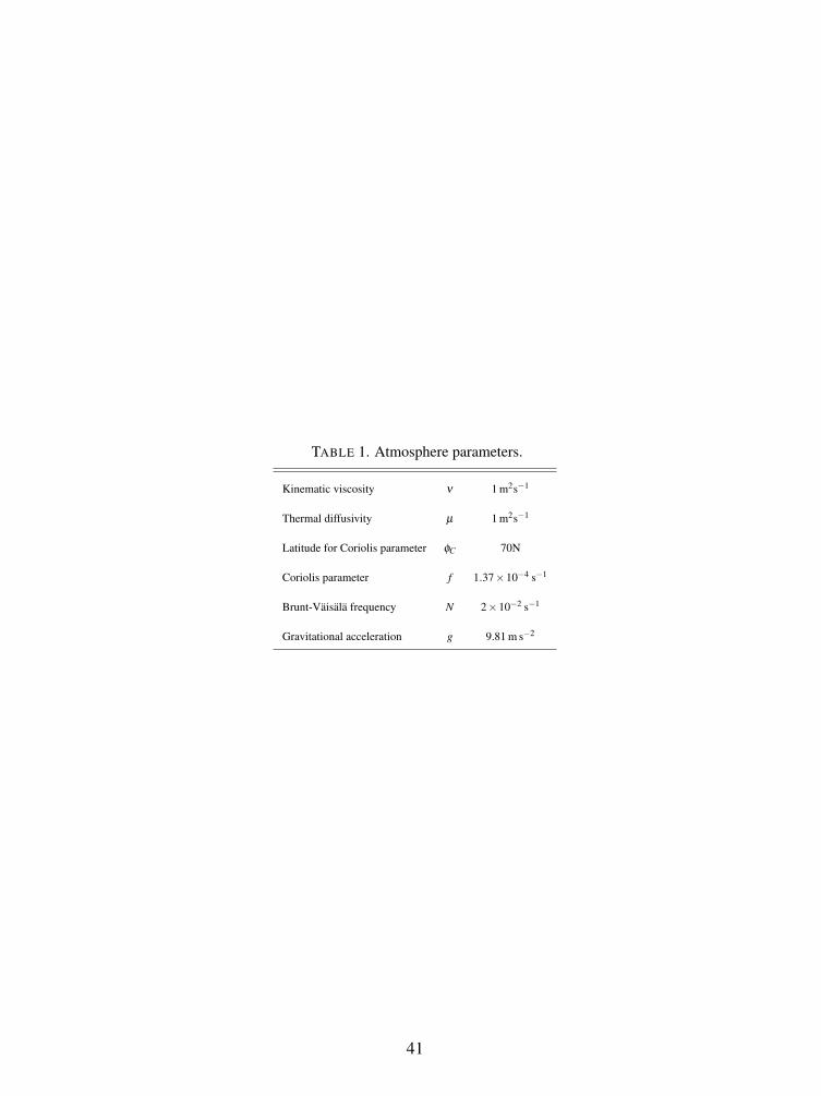
TABLE 1. Atmosphere parameters.

Kinematic viscosity ν 1 m2s−1

Thermal diffusivity µ 1 m2s−1

Latitude for Coriolis parameter φC 70N

Coriolis parameter f 1.37×10−4 s−1

Brunt-Vaisala frequency N 2×10−2 s−1

Gravitational acceleration g 9.81 m s−2

41

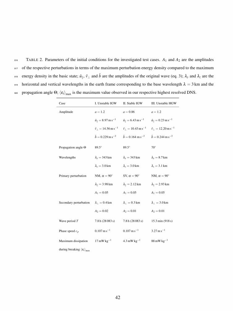
TABLE 2. Parameters of the initial conditions for the investigated test cases. A1 and A2 are the amplitudes

of the respective perturbations in terms of the maximum perturbation energy density compared to the maximum

energy density in the basic state; u‖, v⊥ and b are the amplitudes of the original wave (eq. 3); λy and λz are the

horizontal and vertical wavelengths in the earth frame corresponding to the base wavelength λ = 3 km and the

propagation angle Θ; 〈εt〉max is the maximum value observed in our respective highest resolved DNS.

816

817

818

819

820

Case I. Unstable IGW II. Stable IGW III. Unstable HGW

Amplitude a = 1.2 a = 0.86 a = 1.2

u‖ = 8.97 m s−1 u‖ = 6.43 m s−1 u‖ = 0.23 m s−1

v⊥ = 14.56 m s−1 v⊥ = 10.43 m s−1 v⊥ = 12.20 m s−1

b = 0.229 m s−2 b = 0.164 m s−2 b = 0.244 m s−2

Propagation angle Θ 89.5◦ 89.5◦ 70◦

Wavelengths λy = 343 km λy = 343 km λy = 8.7 km

λz = 3.0 km λz = 3.0 km λz = 3.1 km

Primary perturbation NM, α = 90◦ SV, α = 90◦ NM, α = 90◦

λ‖ = 3.98 km λ‖ = 2.12 km λ‖ = 2.93 km

A1 = 0.05 A1 = 0.05 A1 = 0.05

Secondary perturbation λ⊥ = 0.4 km λ⊥ = 0.3 km λ⊥ = 3.0 km

A2 = 0.02 A2 = 0.01 A2 = 0.01

Wave period T 7.8 h (28 083 s) 7.8 h (28 083 s) 15.3 min (918 s)

Phase speed cp 0.107 m s−1 0.107 m s−1 3.27 m s−1

Maximum dissipation 17 mW kg−1 4.3 mW kg−1 88 mW kg−1

during breaking 〈εt〉max

42

LIST OF FIGURES821

Fig. 1. Rotated coordinate system and computational domain (grey box) for the monochromatic822

gravity wave (after Remmler et al. 2013). . . . . . . . . . . . . . . . 45823

Fig. 2. Initial horizontally (x‖-y⊥) averaged perturbation energy at different 3-D grid resolutions. . . 46824

Fig. 3. Statically unstable IGW (3-D): Base wave amplitudes a and total dissipation rates εt at825

coarse, medium and fine LES resolution. The grey shaded area indicates the standard devi-826

ation of four DNS and the error bars indicate the standard deviation of nine LES. . . . . 47827

Fig. 4. Statically unstable IGW (3-D): Hovmoller plots of horizontally averaged (resolved) dissipa-828

tion of kinetic energy. Top left panel: DNS (640× 64× 500 cells), the other panels: LES829

(100×24×80 cells). The dashed line indicates a fixed position in space. . . . . . . 48830

Fig. 5. Statically unstable IGW (3-D): Comparison of resolved (εm), numerical (εn), parametrised831

(εs) and total (εt) dissipation (left column) and thermal (εp) and total dissipation (right col-832

umn) during the first breaking event (DNS: single simulation, LES: ensemble averages).833

49834

Fig. 6. Statically unstable IGW (3-D): Distributions of total, kinetic and potential energy over ver-835

tical wavelength λζ at the moment of maximum total energy dissipation (left column) and836

at t = 2 hours (right column) (DNS: single simulation, LES: ensemble averages). . . . . 50837

Fig. 7. Statically unstable IGW (2.5-D): Base wave amplitude a and total dissipation rate εt at838

coarse, medium and fine LES resolution compared with a and resolved dissipation rate εm839

from DNS. The grey shaded area indicates the standard deviation of eight DNS, the error840

bars indicate the standard deviation of nine LES. . . . . . . . . . . . . . 51841

Fig. 8. Statically stable IGW (3-D): Base wave amplitude a and total dissipation rate εt at three842

different LES resolutions. The grey shaded area indicates the standard deviation of five843

DNS and the error bars indicate the standard deviation of nine LES. . . . . . . . . 52844

Fig. 9. Statically stable IGW (2.5-D): Base wave amplitude a and total dissipation rate εt at three845

different LES resolutions compared with a and resolved dissipation rate εm from DNS. The846

grey shaded area indicates the standard deviation of six DNS, the error bars indicate the847

standard deviation of nine LES. . . . . . . . . . . . . . . . . . . 53848

Fig. 10. Statically unstable HGW (3-D): Base wave amplitude a and total dissipation rate εt at coarse,849

medium and fine LES resolution. The grey shaded area indicates the standard deviation of850

five DNS, the error bars indicate the standard deviation of nine LES. . . . . . . . . 54851

Fig. 11. Statically unstable HGW (3-D): Comparison of resolved (εm), numerical (εn), parametrised852

(εs) and total (εt) dissipation (left column) and thermal (εp) and total dissipation (right col-853

umn) during the first breaking event (DNS: single simulation, LES: ensemble averages).854

55855

Fig. 12. Statically unstable HGW (3-D): Distributions of total, kinetic and potential energy over856

vertical wavelength λζ at the moment of maximum total energy dissipation (left column)857

and at t = 30 min (right column) (DNS: single simulation, LES: ensemble averages). . . . 56858

Fig. 13. Statically unstable HGW (2.5-D): Base wave amplitude a and total dissipation rate εt at859

coarse, medium and fine LES resolution compared with a and resolved dissipation rate εm860

43

from DNS. The grey shaded area indicates the standard deviation of six DNS, the error bars861

indicate the standard deviation of nine LES. . . . . . . . . . . . . . . 57862

44

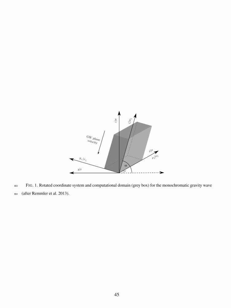
Θ

x|u

x‖|u‖

y|v

y⊥ |v⊥

z|w

ζ|wζ

GW phasevelocity

FIG. 1. Rotated coordinate system and computational domain (grey box) for the monochromatic gravity wave

(after Remmler et al. 2013).

863

864

45

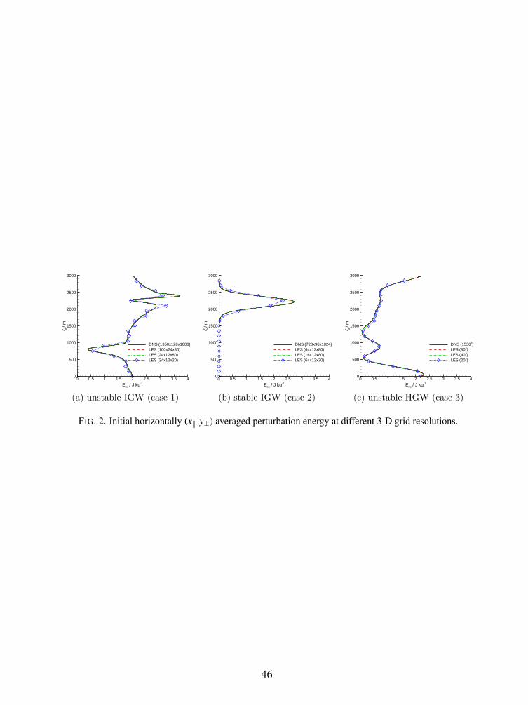
Eini / J kg-1

/ m

0 0.5 1 1.5 2 2.5 3 3.5 40

500

1000

1500

2000

2500

3000

DNS (1350x128x1000)LES (100x24x80)LES (24x12x80)LES (24x12x20)

Eini / J kg-1

/ m

0 0.5 1 1.5 2 2.5 3 3.5 40

500

1000

1500

2000

2500

3000

DNS (720x96x1024)LES (64x12x80)LES (16x12x80)LES (64x12x20)

Eini / J kg-1

/ m

0 0.5 1 1.5 2 2.5 3 3.5 40

500

1000

1500

2000

2500

3000

DNS (15363)LES (803)LES (403)LES (203)

(a) unstable IGW (case 1) (b) stable IGW (case 2) (c) unstable HGW (case 3)

FIG. 2. Initial horizontally (x‖-y⊥) averaged perturbation energy at different 3-D grid resolutions.

46

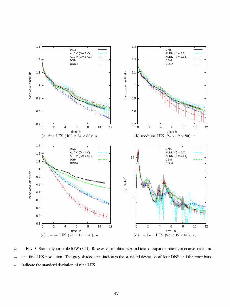
0.7

0.8

0.9

1

1.1

1.2

1.3

0 2 4 6 8 10 12

base

wav

e am

plitu

de

time / h

DNSALDM (β = 0.0)ALDM (β = 0.01)DSMCDS4

0.7

0.8

0.9

1

1.1

1.2

1.3

0 2 4 6 8 10 12ba

se w

ave

ampl

itude

time / h


(a) fine LES (100 × 24 × 80): a (b) medium LES (24 × 12 × 80): a

0.3

0.4

0.5

0.6

0.7

0.8

0.9

1

1.1

1.2

1.3

0 2 4 6 8 10 12

base

wav

e am

plitu

de

time / h


1

10

0 2 4 6 8 10 12

ε t /

mW

kg-1

time / h


(c) coarse LES (24 × 12 × 20): a (d) medium LES (24 × 12 × 80): εt

FIG. 3. Statically unstable IGW (3-D): Base wave amplitudes a and total dissipation rates εt at coarse, medium

and fine LES resolution. The grey shaded area indicates the standard deviation of four DNS and the error bars

indicate the standard deviation of nine LES.

865

866

867

47

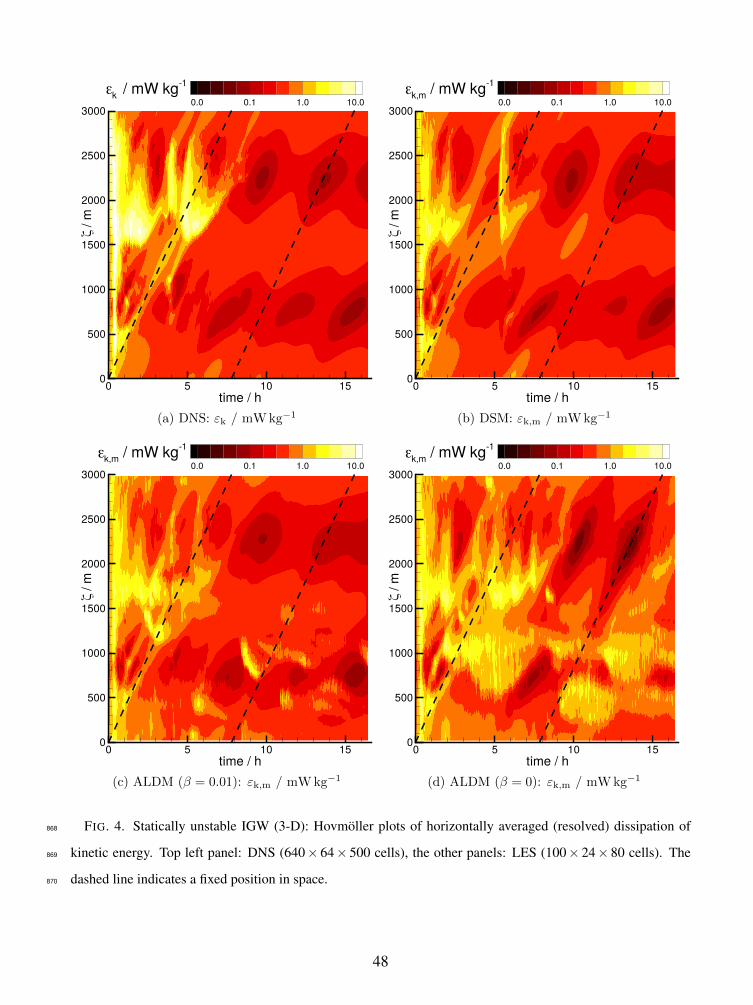
time / h

/ m

0 5 10 150

500

1000

1500

2000

2500

30000.0 0.1 1.0 10.0

kζ

ε / mW kg-1

time / h/ m

0 5 10 150

500

1000

1500

2000

2500

30000.0 0.1 1.0 10.0

k,m

ζ

ε / mW kg-1

(a) DNS: εk / mWkg−1 (b) DSM: εk,m / mWkg−1

time / h

/ m

0 5 10 150

500

1000

1500

2000

2500

30000.0 0.1 1.0 10.0

k,m

ζ

ε / mW kg-1

time / h

/ m

0 5 10 150

500

1000

1500

2000

2500

30000.0 0.1 1.0 10.0

k,m

ζ

ε / mW kg-1

(c) ALDM (β = 0.01): εk,m / mWkg−1 (d) ALDM (β = 0): εk,m / mWkg−1

FIG. 4. Statically unstable IGW (3-D): Hovmoller plots of horizontally averaged (resolved) dissipation of

kinetic energy. Top left panel: DNS (640× 64× 500 cells), the other panels: LES (100× 24× 80 cells). The

dashed line indicates a fixed position in space.

868

869

870

48

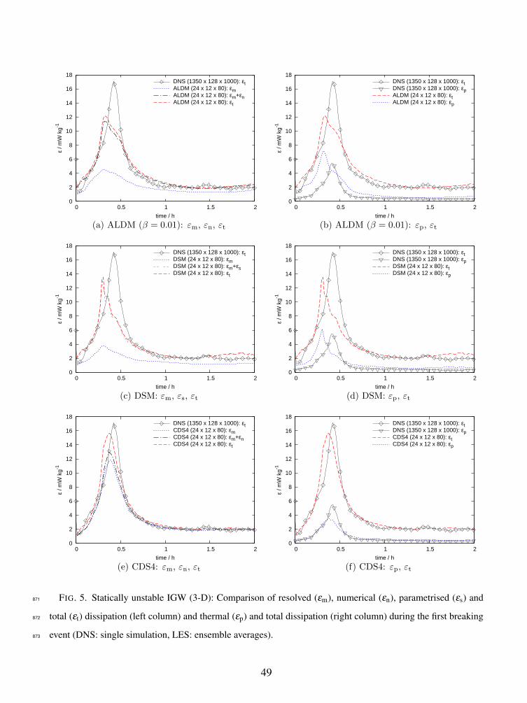
0

2

4

6

8

10

12

14

16

18

0 0.5 1 1.5 2

ε / m

W k

g-1

time / h

DNS (1350 x 128 x 1000): εtALDM (24 x 12 x 80): εmALDM (24 x 12 x 80): εm+εnALDM (24 x 12 x 80): εt

0

2

4

6

8

10

12

14

16

18

0 0.5 1 1.5 2

ε / m

W k

g-1

time / h

DNS (1350 x 128 x 1000): εtDNS (1350 x 128 x 1000): εpALDM (24 x 12 x 80): εtALDM (24 x 12 x 80): εp

(a) ALDM (β = 0.01): εm, εn, εt (b) ALDM (β = 0.01): εp, εt

0

2

4

6

8

10

12

14

16

18

0 0.5 1 1.5 2

ε / m

W k

g-1

time / h

DNS (1350 x 128 x 1000): εtDSM (24 x 12 x 80): εmDSM (24 x 12 x 80): εm+εsDSM (24 x 12 x 80): εt

0

2

4

6

8

10

12

14

16

18

0 0.5 1 1.5 2

ε / m

W k

g-1

time / h

DNS (1350 x 128 x 1000): εtDNS (1350 x 128 x 1000): εpDSM (24 x 12 x 80): εtDSM (24 x 12 x 80): εp

(c) DSM: εm, εs, εt (d) DSM: εp, εt

0

2

4

6

8

10

12

14

16

18

0 0.5 1 1.5 2

ε / m

W k

g-1

time / h

DNS (1350 x 128 x 1000): εtCDS4 (24 x 12 x 80): εmCDS4 (24 x 12 x 80): εm+εnCDS4 (24 x 12 x 80): εt

0

2

4

6

8

10

12

14

16

18

0 0.5 1 1.5 2

ε / m

W k

g-1

time / h

DNS (1350 x 128 x 1000): εtDNS (1350 x 128 x 1000): εpCDS4 (24 x 12 x 80): εtCDS4 (24 x 12 x 80): εp

(e) CDS4: εm, εn, εt (f) CDS4: εp, εt

FIG. 5. Statically unstable IGW (3-D): Comparison of resolved (εm), numerical (εn), parametrised (εs) and

total (εt) dissipation (left column) and thermal (εp) and total dissipation (right column) during the first breaking

event (DNS: single simulation, LES: ensemble averages).

871

872

873

49

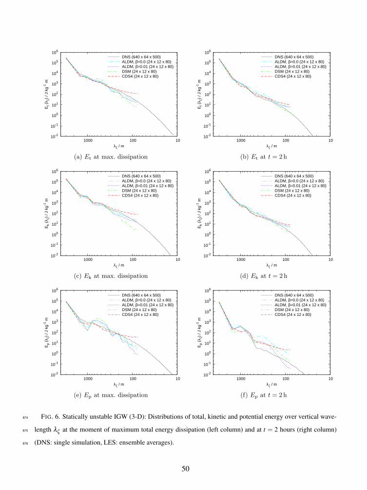
10-2

10-1

100

101

102

103

104

105

106

10 100 1000

Et (

λ ζ)

/ J k

g-1 m

λζ / m

DNS (640 x 64 x 500)ALDM, β=0.0 (24 x 12 x 80)ALDM, β=0.01 (24 x 12 x 80)DSM (24 x 12 x 80)CDS4 (24 x 12 x 80)

10-2

10-1

100

101

102

103

104

105

106

10 100 1000

Et (

λ ζ)

/ J k

g-1 m

λζ / m


(a) Et at max. dissipation (b) Et at t = 2h

10-2

10-1

100

101

102

103

104

105

106

10 100 1000

Ek

(λζ)

/ J

kg-1

m

λζ / m


10-2

10-1

100

101

102

103

104

105

106

10 100 1000

Ek

(λζ)

/ J

kg-1

m

λζ / m


(c) Ek at max. dissipation (d) Ek at t = 2h

10-2

10-1

100

101

102

103

104

105

106

10 100 1000

Ep

(λζ)

/ J

kg-1

m

λζ / m


10-2

10-1

100

101

102

103

104

105

106

10 100 1000

Ep

(λζ)

/ J

kg-1

m

λζ / m


(e) Ep at max. dissipation (f) Ep at t = 2h

FIG. 6. Statically unstable IGW (3-D): Distributions of total, kinetic and potential energy over vertical wave-

length λζ at the moment of maximum total energy dissipation (left column) and at t = 2 hours (right column)

(DNS: single simulation, LES: ensemble averages).

874

875

876

50

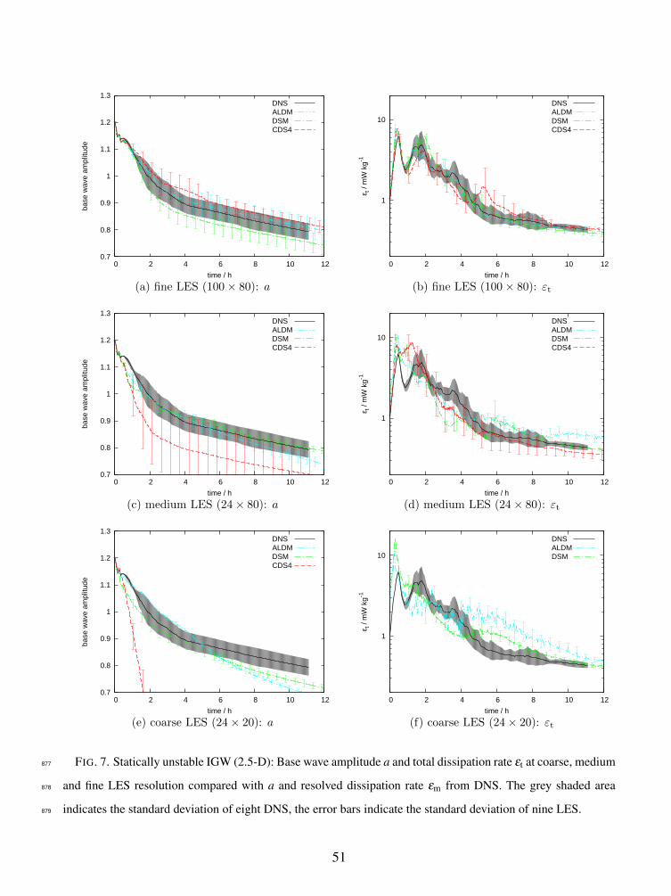
0.7

0.8

0.9

1

1.1

1.2

1.3

0 2 4 6 8 10 12

base

wav

e am

plitu

de

time / h

DNSALDMDSMCDS4

1

10

0 2 4 6 8 10 12

ε t /

mW

kg-1

time / h

DNSALDMDSMCDS4

(a) fine LES (100 × 80): a (b) fine LES (100 × 80): εt

0.7

0.8

0.9

1

1.1

1.2

1.3

0 2 4 6 8 10 12

base

wav

e am

plitu

de

time / h

DNSALDMDSMCDS4

1

10

0 2 4 6 8 10 12

ε t /

mW

kg-1

time / h

DNSALDMDSMCDS4

(c) medium LES (24 × 80): a (d) medium LES (24 × 80): εt

0.7

0.8

0.9

1

1.1

1.2

1.3

0 2 4 6 8 10 12

base

wav

e am

plitu

de

time / h

DNSALDMDSMCDS4

1

10

0 2 4 6 8 10 12

ε t /

mW

kg-1

time / h

DNSALDMDSM

(e) coarse LES (24 × 20): a (f) coarse LES (24 × 20): εt

FIG. 7. Statically unstable IGW (2.5-D): Base wave amplitude a and total dissipation rate εt at coarse, medium

and fine LES resolution compared with a and resolved dissipation rate εm from DNS. The grey shaded area

indicates the standard deviation of eight DNS, the error bars indicate the standard deviation of nine LES.

877

878

879

51

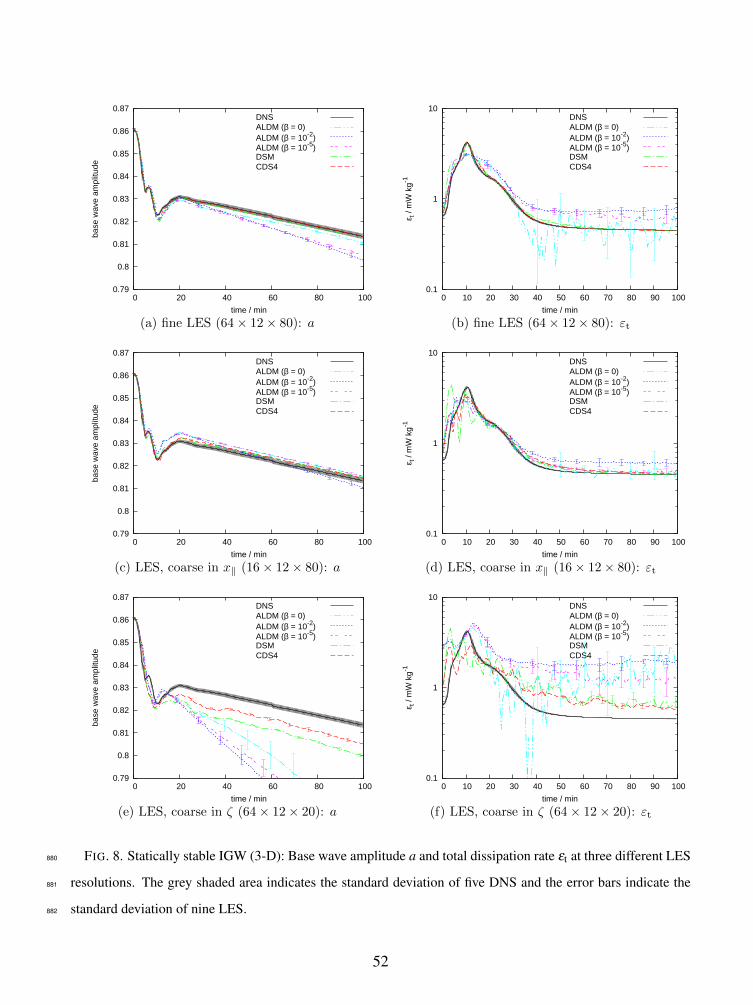
0.79

0.8

0.81

0.82

0.83

0.84

0.85

0.86

0.87

0 20 40 60 80 100

base

wav

e am

plitu

de

time / min

DNSALDM (β = 0)ALDM (β = 10-2)ALDM (β = 10-5)DSMCDS4

0.1

1

10

0 10 20 30 40 50 60 70 80 90 100

ε t /

mW

kg-1

time / min


(a) fine LES (64 × 12 × 80): a (b) fine LES (64 × 12 × 80): εt

0.79

0.8

0.81

0.82

0.83

0.84

0.85

0.86

0.87

0 20 40 60 80 100

base

wav

e am

plitu

de

time / min


0.1

1

10

0 10 20 30 40 50 60 70 80 90 100

ε t /

mW

kg-1

time / min


(c) LES, coarse in x‖ (16 × 12 × 80): a (d) LES, coarse in x‖ (16 × 12 × 80): εt

0.79

0.8

0.81

0.82

0.83

0.84

0.85

0.86

0.87

0 20 40 60 80 100

base

wav

e am

plitu

de

time / min


0.1

1

10

0 10 20 30 40 50 60 70 80 90 100

ε t /

mW

kg-1

time / min


(e) LES, coarse in ζ (64 × 12 × 20): a (f) LES, coarse in ζ (64 × 12 × 20): εt

FIG. 8. Statically stable IGW (3-D): Base wave amplitude a and total dissipation rate εt at three different LES

resolutions. The grey shaded area indicates the standard deviation of five DNS and the error bars indicate the

standard deviation of nine LES.

880

881

882

52

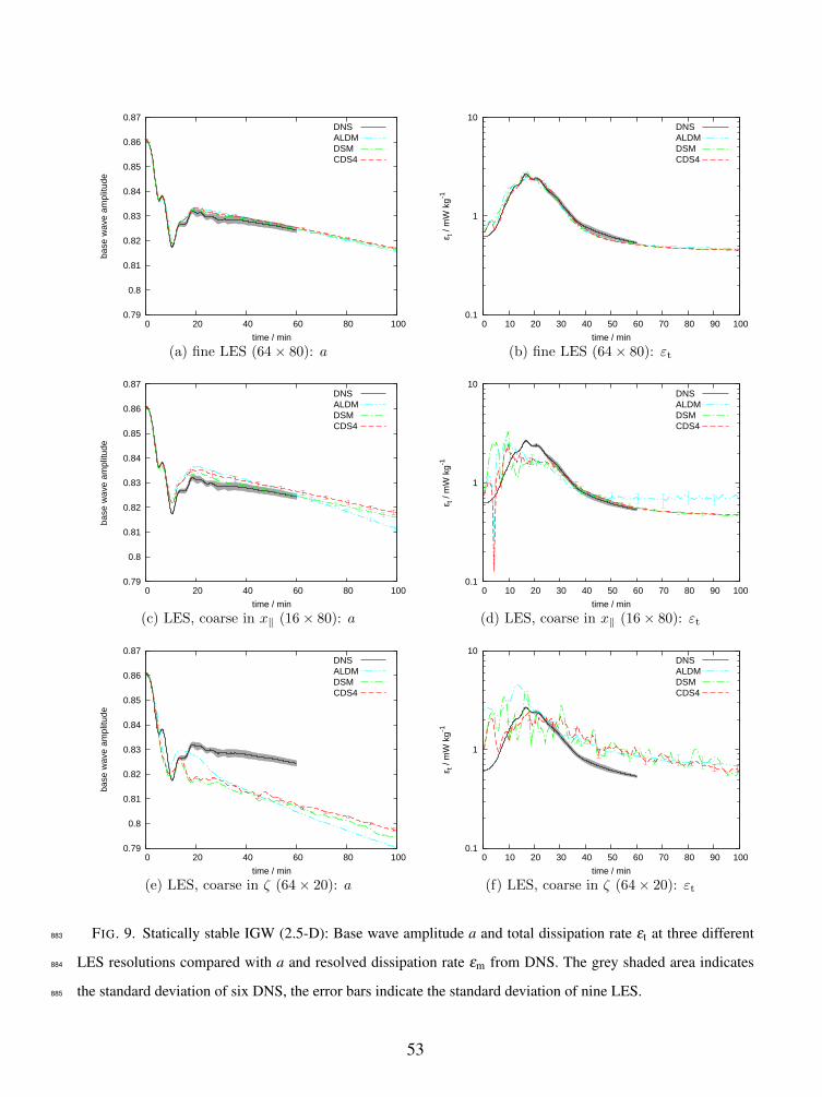
0.79

0.8

0.81

0.82

0.83

0.84

0.85

0.86

0.87

0 20 40 60 80 100

base

wav

e am

plitu

de

time / min

DNSALDMDSMCDS4

0.1

1

10

0 10 20 30 40 50 60 70 80 90 100

ε t /

mW

kg-1

time / min

DNSALDMDSMCDS4

(a) fine LES (64 × 80): a (b) fine LES (64 × 80): εt

0.79

0.8

0.81

0.82

0.83

0.84

0.85

0.86

0.87

0 20 40 60 80 100

base

wav

e am

plitu

de

time / min

DNSALDMDSMCDS4

0.1

1

10

0 10 20 30 40 50 60 70 80 90 100

ε t /

mW

kg-1

time / min

DNSALDMDSMCDS4

(c) LES, coarse in x‖ (16 × 80): a (d) LES, coarse in x‖ (16 × 80): εt

0.79

0.8

0.81

0.82

0.83

0.84

0.85

0.86

0.87

0 20 40 60 80 100

base

wav

e am

plitu

de

time / min

DNSALDMDSMCDS4

0.1

1

10

0 10 20 30 40 50 60 70 80 90 100

ε t /

mW

kg-1

time / min

DNSALDMDSMCDS4

(e) LES, coarse in ζ (64 × 20): a (f) LES, coarse in ζ (64 × 20): εt

FIG. 9. Statically stable IGW (2.5-D): Base wave amplitude a and total dissipation rate εt at three different

LES resolutions compared with a and resolved dissipation rate εm from DNS. The grey shaded area indicates

the standard deviation of six DNS, the error bars indicate the standard deviation of nine LES.

883

884

885

53

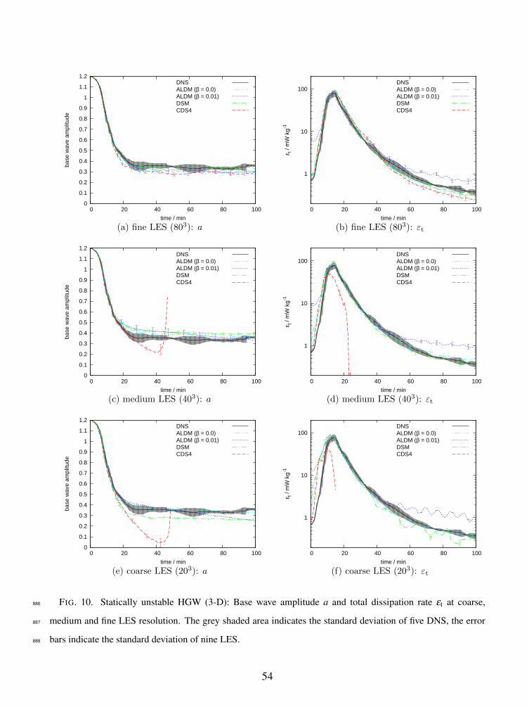
0

0.1

0.2

0.3

0.4

0.5

0.6

0.7

0.8

0.9

1

1.1

1.2

0 20 40 60 80 100

base

wav

e am

plitu

de

time / min


1

10

100

0 20 40 60 80 100

ε t /

mW

kg-1

time / min


(a) fine LES (803): a (b) fine LES (803): εt

0

0.1

0.2

0.3

0.4

0.5

0.6

0.7

0.8

0.9

1

1.1

1.2

0 20 40 60 80 100

base

wav

e am

plitu

de

time / min


1

10

100

0 20 40 60 80 100

ε t /

mW

kg-1

time / min


(c) medium LES (403): a (d) medium LES (403): εt

0

0.1

0.2

0.3

0.4

0.5

0.6

0.7

0.8

0.9

1

1.1

1.2

0 20 40 60 80 100

base

wav

e am

plitu

de

time / min


1

10

100

0 20 40 60 80 100

ε t /

mW

kg-1

time / min


(e) coarse LES (203): a (f) coarse LES (203): εt

FIG. 10. Statically unstable HGW (3-D): Base wave amplitude a and total dissipation rate εt at coarse,

medium and fine LES resolution. The grey shaded area indicates the standard deviation of five DNS, the error

bars indicate the standard deviation of nine LES.

886

887

888

54

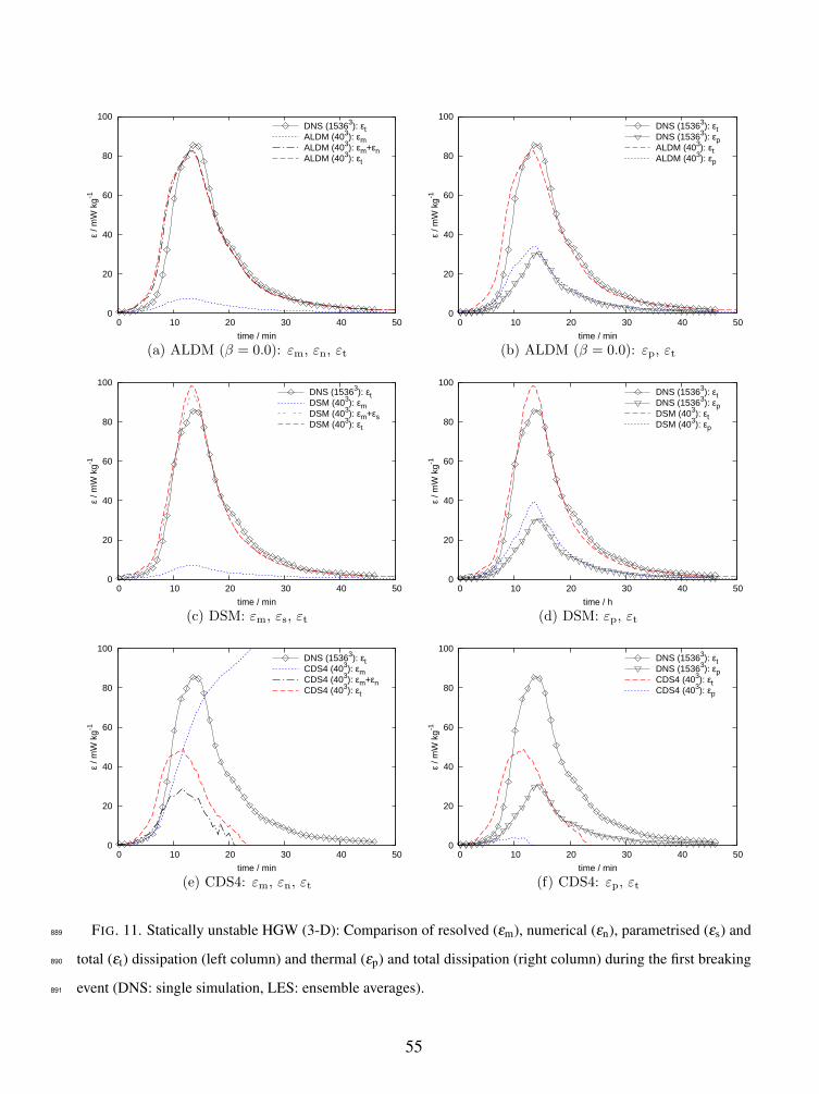
0

20

40

60

80

100

0 10 20 30 40 50

ε / m

W k

g-1

time / min

DNS (15363): εtALDM (403): εmALDM (403): εm+εnALDM (403): εt

0

20

40

60

80

100

0 10 20 30 40 50

ε / m

W k

g-1

time / min

DNS (15363): εtDNS (15363): εpALDM (403): εtALDM (403): εp

(a) ALDM (β = 0.0): εm, εn, εt (b) ALDM (β = 0.0): εp, εt

0

20

40

60

80

100

0 10 20 30 40 50

ε / m

W k

g-1

time / min

DNS (15363): εtDSM (403): εmDSM (403): εm+εsDSM (403): εt

0

20

40

60

80

100

0 10 20 30 40 50

ε / m

W k

g-1

time / h

DNS (15363): εtDNS (15363): εpDSM (403): εtDSM (403): εp

(c) DSM: εm, εs, εt (d) DSM: εp, εt

0

20

40

60

80

100

0 10 20 30 40 50

ε / m

W k

g-1

time / min

DNS (15363): εtCDS4 (403): εmCDS4 (403): εm+εnCDS4 (403): εt

0

20

40

60

80

100

0 10 20 30 40 50

ε / m

W k

g-1

time / min

DNS (15363): εtDNS (15363): εpCDS4 (403): εtCDS4 (403): εp

(e) CDS4: εm, εn, εt (f) CDS4: εp, εt

FIG. 11. Statically unstable HGW (3-D): Comparison of resolved (εm), numerical (εn), parametrised (εs) and

total (εt) dissipation (left column) and thermal (εp) and total dissipation (right column) during the first breaking

event (DNS: single simulation, LES: ensemble averages).

889

890

891

55

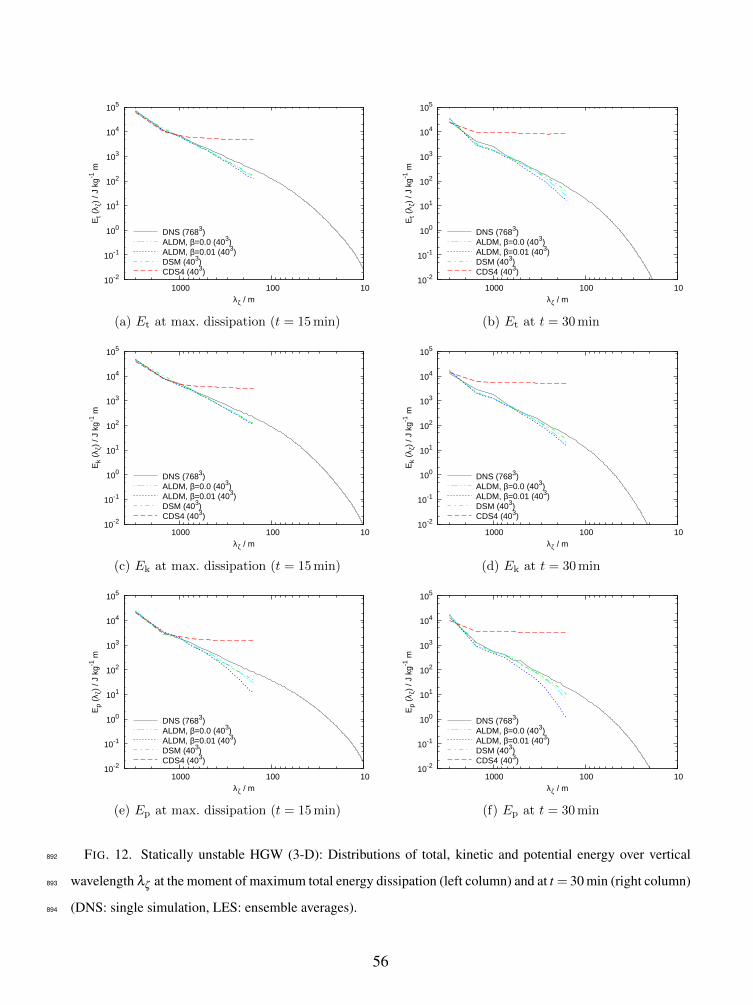
10-2

10-1

100

101

102

103

104

105

10 100 1000

Et (

λ ζ)

/ J k

g-1 m

λζ / m

DNS (7683)ALDM, β=0.0 (403)ALDM, β=0.01 (403)DSM (403)CDS4 (403)

10-2

10-1

100

101

102

103

104

105

10 100 1000

Et (

λ ζ)

/ J k

g-1 m

λζ / m


(a) Et at max. dissipation (t = 15min) (b) Et at t = 30min

10-2

10-1

100

101

102

103

104

105

10 100 1000

Ek

(λζ)

/ J

kg-1

m

λζ / m


10-2

10-1

100

101

102

103

104

105

10 100 1000

Ek

(λζ)

/ J

kg-1

m

λζ / m


(c) Ek at max. dissipation (t = 15min) (d) Ek at t = 30min

10-2

10-1

100

101

102

103

104

105

10 100 1000

Ep

(λζ)

/ J

kg-1

m

λζ / m


10-2

10-1

100

101

102

103

104

105

10 100 1000

Ep

(λζ)

/ J

kg-1

m

λζ / m


(e) Ep at max. dissipation (t = 15min) (f) Ep at t = 30min

FIG. 12. Statically unstable HGW (3-D): Distributions of total, kinetic and potential energy over vertical

wavelength λζ at the moment of maximum total energy dissipation (left column) and at t = 30 min (right column)

(DNS: single simulation, LES: ensemble averages).

892

893

894

56

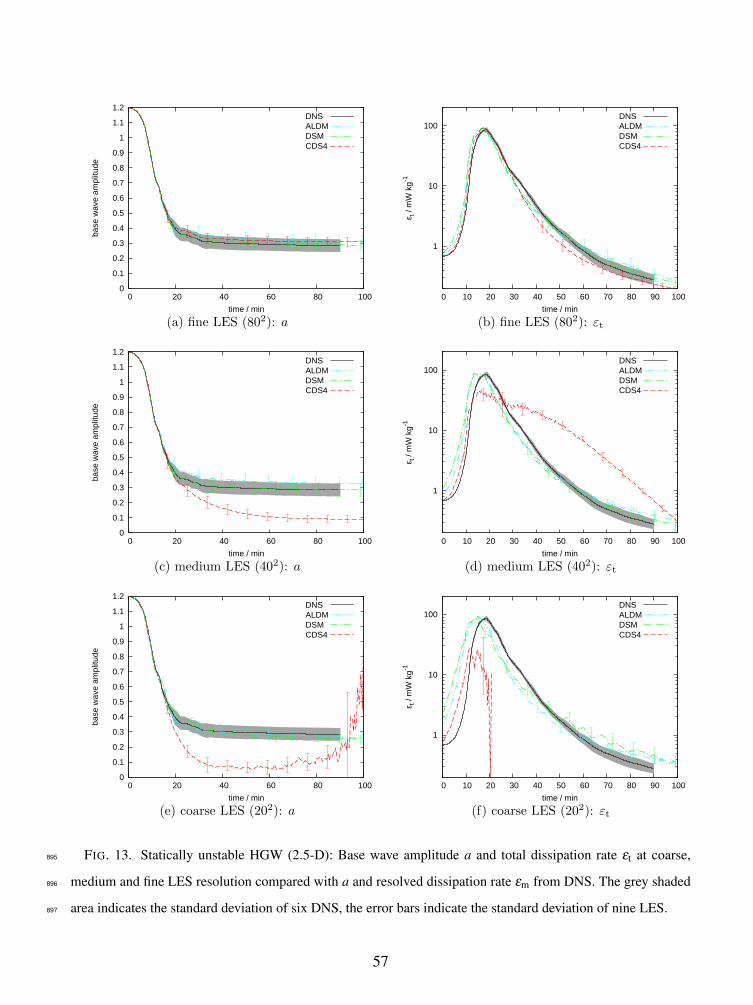
0

0.1

0.2

0.3

0.4

0.5

0.6

0.7

0.8

0.9

1

1.1

1.2

0 20 40 60 80 100

base

wav

e am

plitu

de

time / min

DNSALDMDSMCDS4

1

10

100

0 10 20 30 40 50 60 70 80 90 100

ε t /

mW

kg-1

time / min

DNSALDMDSMCDS4

(a) fine LES (802): a (b) fine LES (802): εt

0

0.1

0.2

0.3

0.4

0.5

0.6

0.7

0.8

0.9

1

1.1

1.2

0 20 40 60 80 100

base

wav

e am

plitu

de

time / min

DNSALDMDSMCDS4

1

10

100

0 10 20 30 40 50 60 70 80 90 100

ε t /

mW

kg-1

time / min

DNSALDMDSMCDS4

(c) medium LES (402): a (d) medium LES (402): εt

0

0.1

0.2

0.3

0.4

0.5

0.6

0.7

0.8

0.9

1

1.1

1.2

0 20 40 60 80 100

base

wav

e am

plitu

de

time / min

DNSALDMDSMCDS4

1

10

100

0 10 20 30 40 50 60 70 80 90 100

ε t /

mW

kg-1

time / min

DNSALDMDSMCDS4

(e) coarse LES (202): a (f) coarse LES (202): εt

FIG. 13. Statically unstable HGW (2.5-D): Base wave amplitude a and total dissipation rate εt at coarse,

medium and fine LES resolution compared with a and resolved dissipation rate εm from DNS. The grey shaded

area indicates the standard deviation of six DNS, the error bars indicate the standard deviation of nine LES.

895

896

897

57

Documents

1 Validation of Large-Eddy Simulation Methods for Gravity