Embed Size (px)
Citation preview
1
Ultracold atoms in optical lattices
In this chapter we introduce the reader to the physics of ultracold atoms
trapped in crystals made of light: optical lattices. The chapter begins with
a review of the foundations of atom-light interactions and explains how
those interactions can be used to trap and manipulate atoms. Then it takes
a route through the basic physics describing the behavior of cold atoms
trapped in optical lattices. It starts with the simple noninteracting regime,
where important concepts such as band structure, Bloch waves and Wannier
functions are introduced, and then goes into the the strongly interacting
regime where new states of matter such as the so called Mott insulator
state emerge. The chapter discusses standard theoretical methods commonly
used to deal with interacting systems and apply them to calculate the phase
diagram of the Bose Hubbard model which describes bosonic atoms hopping
in a lattice and interacting only when more than two occupy the same lattice
site. In the following chapter we will use the techniques introduced here to
compute quantum correlations and other many body properties.
1.1 Optical lattices
Optical lattices are artificial crystals of light created by interfering optical
laser beams. When atoms are illuminated with laser beams, the electric field
of the laser induces a dipole moment in the atoms which in turn interacts
with the electric field. This interaction modifies the energy of the internal
states of the atoms in a way that depends both on the light intensity and
on the laser frequency. A spatially dependent intensity induces a spatially
dependent potential energy which can be used to trap the atoms. An optical
lattice is the periodic potential energy landscape that the atoms experience
as a result of the standing wave pattern generated by the interference of
laser beams.

2 Ultracold atoms in optical lattices
Optical Lattices
• Fully controllable, no
defects, no vibrations
• Lattice spacing
micrometers
• Trapped atom mass ~
10-100 amu
• Temperature :
T~1 nK
Solid state crystals
• Very complex condensed
matter environment
• Lattice spacing
Angstroms
• Electron mass 1/1900
amu
• Temperature :
T~ 100 K
Atoms ↔ Electrons
Optical lattice ↔ Ionic Crystal
Figure 1.1 Optical lattice vs solid state crystal lattices. Atoms trapped inoptical lattices can be used to mimic the behavior of conduction electronsin solid state crystals.
Optical lattices have been widely used in atomic physics as a way to
cool, trap and control atoms. In the recent years ultracold atoms in optical
lattices have become a unique meeting ground for simulating solid state ma-
terials [Bloch et al. (2008)]. The optical lattice potential mimics the crystal
lattice in a solid and the atoms loaded in the lattice mimic the valence elec-
trons (See figure 1.2). Atoms move in the lattice (actually tunnel quantum-
mechanically between lattice sites) as valence electrons do in the periodic
energy landscape generated by the positively charged ions in a solid crystal.
There are, however, some important difference between solid-state crystals
and optical lattice which are relevant to emphasize. First of all the energy
scales in consideration are very different. While the typical lattice spacing
in cold atoms systems is of the order of one µm, in solid-state crystals it is
around 0.1 nm. Atoms are also much heavier than electrons. That means that
to probe the same physics that occurs at 100 kelvin temperatures in solid-
1.1 Optical lattices 3
state systems we need to cool to atoms below a few nanokelvin. The much
lower energy scale requires the need of state-of-the-art cooling techniques
but is advantageous for probing. Ultra-cold atomic systems do not require
sophisticated ultra-fast probes. In such systems it is possible to follow the
dynamics of the atoms on the time scales of ms or even seconds. Moreover, in
contrast to electrons which are charged particles and strongly coupled to the
complex solid-state environment, atoms are neutral and almost completely
decoupled from their environment. In contrast to real materials where dis-
order, lattice vibrations and structural defects are inevitable, crystals made
by light are rigid (no vibrations), free of defects and fully controllable.
The lattice geometry is determined by the configuration of laser beams
used to create the lattice and the lattice depth is tunable by the laser inten-
sity. There is even flexibility in controlling the lattice spacing by modifying
the interference angle between the laser beams. By controlling the intensity
of the trapping laser beams the dimensionality of the system can be var-
ied from 3D to 0D even dynamically during the course of an experiment.
Thanks to all these attributes ultra-cold atoms loaded in optical lattice
have become a perfect arena for the investigation of non-linear phenomena,
quantum phase transitions and non-equilibrium dynamics. Atoms loaded
in optical lattices have also been proposed as ideal quantum information
processors.
1.1.1 Basic Theory of optical lattices
Let us first start by explaining in more detail how optical lattice potentials
are generated. Neutral atoms interact with light in both dissipative and con-
servative ways. The conservative interaction comes from the interaction of
the light field with the induced dipole moment of the atom which causes a
shift in the potential energy called AC-Stark shift. The dissipative interac-
tion comes due to the absorption of photons followed by spontaneous emis-
sion. Laser cooling techniques make use of this dissipative process [Phillips
(1998)]. In this chapter we will mainly concentrate on the conservative part
of the interaction and just briefly mention the the basic origin and conse-
quences of the dissipative part.
AC Stark Shift
Consider a two level atom, with internal ground state |g〉 and excited state
|e〉 separated by an energy hω0. The atom is illuminated with a classical
electromagnetic field E = E(x)e−iωt + E∗(x)eiωt with amplitude E(x) and
angular frequency ω = 2πν as schematically shown in Fig.1.2.
4 Ultracold atoms in optical lattices
Periodic light shift potentials for atoms created by the
interference of multiple laser beams.
Two counter-propagating beams
Standing wave
|e
hn
|g
d
d
~
d=l/2
~Intensity Ω2
𝛿
𝑉 𝑥 ~Ω0
2
𝛿sin(𝑘𝑥)
Figure 1.2 AC Stark shift induced by atom-light interaction. The laserfrequency is ω = 2πν which is detuned from the atomic resonance by δ
The electromagnetic field induces a dipole moment in the atom, d, which
interacts with it in the usual way:
V = −d ·E (1.1)
Quantum mechanically the dipole moment is an operator and can be writ-
ten in the two level atom basis as: d =∑
α,β=e,g〈α|d|β〉|α〉〈β|. Note that∑α |α〉〈α| = 1. Since atoms do not have a permanent dipole moment,
〈α|d|α〉 = 0, and only the off-diagonal terms are non-zero µeg = 〈e|d|g〉 6= 0.
Those determine the induced dipole moment. This means that d = µeg|e〉〈g|+µ∗eg|g〉〈e|, and the total Hamiltonian of the system can be written as:
H = hω0 |e〉 〈e| −(µeg|e〉〈g|+ µ∗eg|g〉〈e|
)·(E(x)e−iωt + E∗(x)eiωt
),(1.2)
When the laser detuning δ = ω − ω0 is small, |δ| |ω − ω0|, a conve-
nient way to proceed is to make the Hamiltonian time independent by
going to the rotating frame of the laser. The Hamiltonian in this rotat-
ing frame, determined by the unitary transformation U(t) = e−iωtσz/2 with
σz = |e〉〈e| − |g〉〈g| the corresponding Pauli matrix in the e, g basis, trans-
forms to H → U †HU + ih∂U†
∂t U . After neglecting processes with a rapidly
oscillating phase, exp(−i(ω0 +ω)t) which average out over time, the Hamil-
tonian becomes
1.1 Optical lattices 5
H = − hδ2σz −
(hΩ(~x)
2|e〉 〈g|+ hΩ∗(~x)
2|e〉 〈g|
), (1.3)
where Ω(x) is the so called Rabi frequency given by hΩ(x) = 2E(x) · µge.If the detuning is large compared to the Rabi frequency, |δ| Ω, the effect
of the atom-light interactions on the states |e〉 and |g〉 can be determined
with second order perturbation theory. In this case, the energy shift E(2)g,e is
given by
E(2)g,e = ±| 〈e| H |g〉 |
2
hδ= ±hΩ(x)2
4δ, (1.4)
with the plus and minus sign for the |g〉 and |e〉 states respectively. This
energy shift, hΩ(x)2
4δ is the so called ac-Stark shift and defines the optical
potential that atoms in the state |g〉 experience the g atoms feel due to their
interaction with light. If instead of interacting with an single electromagnetic
field, the atoms are illuminated with superimposed counter propagating laser
beams which interfere, the atoms will feel the standing wave pattern result-
ing from the interference. This periodic landscape modulation of the energy
experienced by the atoms is the so-called optical lattice potential.
In the above discussion we implicitly assumed that the excited state has an
infinite life time. However, in reality it will decay by spontaneous emission
of photons. This effect can be taken into account phenomenologically by
attributing to the excited state an energy with both real and imaginary
parts. If the excited state has a life time 1/Γe, the energy of the perturbed
ground state becomes a complex quantity which we can write as
E(2)g =
h
4
Ω(x)2
δ − iΓe/2= V (x) + iγsc(x), (1.5)
V (x) = hΩ(x)2δ
4δ2 − Γ2e
≈ hΩ(x)2
4δ, γsc(x) =
h
2
Ω(x)2Γe4δ2 − Γ2
e
≈ hΩ(x)2Γe8δ2
.(1.6)
The real part of the energy corresponds to the optical potential V (x). The
sign of the optical potential seen by the atoms depend on the sign of the
detuning. For blue detuning , δ > 0, the sign is positive resulting in a
repulsive potential. The potential minima corresponds to the points with
zero light intensity. Atoms are repealed from the high intensity regions. On
the other hand, in a red detuned light field, δ < 0, the potential is attractive,
the minima correspond to the places with maximum light intensity where
atoms want to stay at. One will often find in the literature the description of
atoms as “weak field seekers” or “strong field seekers” for cases of blue and
red detuning, respectively. The imaginary part, γsc(x) represents the the loss
6 Ultracold atoms in optical lattices
rate of atoms from the ground state. For large detunings the conservative
part of the optical potential dominates and can be used to trap the atoms.
Lattice Geometry
The simplest possible lattice is a one dimensional lattice (1D) lattice.
It can be generated by creating a standing wave interference pattern by
retro reflection of a single laser beam with Rabi frequency Ω0. This results
in a Rabi frequency Ω(x) = 2Ω0 sin(kx) which yields a periodic trapping
potential given by
Vlat(x) = V0 sin2(kx) =hΩ2
0
δsin2(kx) (1.7)
where k = 2π/λ is the magnitude of the laser-light wave vector and V0 is
the lattice depth. This potential has a lattice constant, a, defined by the
condition Vlat(x+ a) = Vlat(x) for all x. This lattice constant is a = λ/2.
Note that mimicking solid state crystals with an optical lattice has the
great advantage that, in general, the lattice geometry can be controlled easily
by changing the laser fields.
Periodic potentials in higher dimensions can be created by superimposing
more laser beams. To create a two dimensional lattice potential for example,
two orthogonal sets of counter propagating laser beams can be used. In this
case the lattice potential has the form
Vlat(x, y) = Vo(cos2(ky) + cos2(kx) + 2ε1 · ε2 cosφ cos(ky) cos(kx)
), (1.8)
Here k is the wave vector magnitude, ε1 and ε2 are polarization vectors of the
counter propagating set and φ is the phase between them. A simple square
lattice can be created by choosing orthogonal polarizations between the
standing waves. In this case the interference term vanishes and the resulting
potential is just the sum of two superimposed 1D lattice potentials. Even
if the polarization of the two pair of beams is the same, they can be made
independent by detuning the common frequency of one pair of beams from
that the other.
A more general class of two 2D lattices can be created from the interference
of three laser beams [Blakie and Porto (2004); Sebby-Strabley et al. (2006);
Wirth et al. (2011); Soltan-Panahi et al. (2011); Tarruell et al. (2012); Jo
et al. (2012)] which in general yield non-separable lattices. Such lattices can
provide better control over the number of nearest neighbors and allow for
the exploration of richer physics. In Fig. 1.3 we show a variety of possible
2D optical lattice geometries that can be made by three and four interfering
laser beams. Different type of lattice potentials can be created in 3D by the
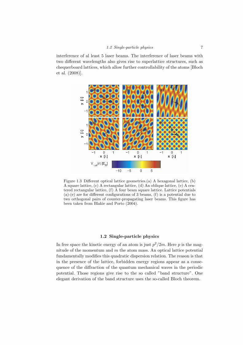
1.2 Single-particle physics 7
interference of al least 5 laser beams. The interference of laser beams with
two different wavelengths also gives rise to superlattice structures, such as
chequerboard lattices, which allow further controllability of the atoms [Bloch
et al. (2008)].
Figure 1.3 Different optical lattice geometries.(a) A hexagonal lattice, (b)A square lattice, (c) A rectangular lattice, (d) An oblique lattice, (e) A cen-tered rectangular lattice, (f) A four beam square lattice. Lattice potentials(a)-(e) are for different configurations of 3 beams, (f) is a potential due totwo orthogonal pairs of counter-propagating laser beams. This figure hasbeen taken from Blakie and Porto (2004).
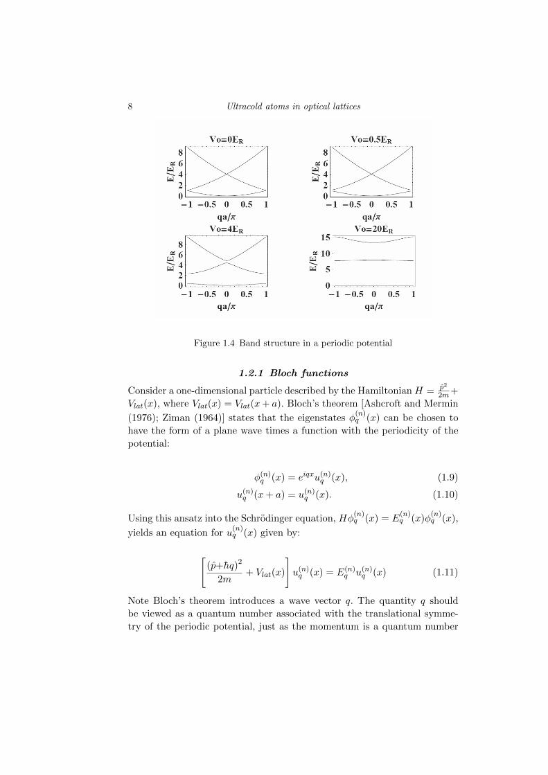
1.2 Single-particle physics
In free space the kinetic energy of an atom is just p2/2m. Here p is the mag-
nitude of the momentum and m the atom mass. An optical lattice potential
fundamentally modifies this quadratic dispersion relation. The reason is that
in the presence of the lattice, forbidden energy regions appear as a conse-
quence of the diffraction of the quantum mechanical waves in the periodic
potential. Those regions give rise to the so called ”band structure”. One
elegant derivation of the band structure uses the so-called Bloch theorem.
8 Ultracold atoms in optical lattices
Figure 1.4 Band structure in a periodic potential
1.2.1 Bloch functions
Consider a one-dimensional particle described by the Hamiltonian H = p2
2m+
Vlat(x), where Vlat(x) = Vlat(x+ a). Bloch’s theorem [Ashcroft and Mermin
(1976); Ziman (1964)] states that the eigenstates φ(n)q (x) can be chosen to
have the form of a plane wave times a function with the periodicity of the
potential:
φ(n)q (x) = eiqxu(n)
q (x), (1.9)
u(n)q (x+ a) = u(n)
q (x). (1.10)
Using this ansatz into the Schrodinger equation, Hφ(n)q (x) = E
(n)q (x)φ
(n)q (x),
yields an equation for u(n)q (x) given by:
[(p+hq)2
2m+ Vlat(x)
]u(n)q (x) = E(n)
q u(n)q (x) (1.11)
Note Bloch’s theorem introduces a wave vector q. The quantity q should
be viewed as a quantum number associated with the translational symme-
try of the periodic potential, just as the momentum is a quantum number
1.2 Single-particle physics 9
associated with the full translational symmetry of free space. It turns out
that, in the presence of a periodic potential, hq plays the same fundamental
role in the dynamics as does the momentum in free space. To emphasize
this similarity hq is called the quasimomentum or crystal momentum . In
general the wave vector q is confined to the first Brilloiun zone, a uniquely
defined primitive cell in momentum space. In 1D systems the Brilloiun zone
corresponds to −K/2 < q ≤ K/2. K = 2π/a is the so called reciprocal
lattice vector.
The index n (band index), appears in Bloch’s theorem because for a given
q there are many solutions to the Schrodinger equation. Eq. (1.11) can be
seen as a set of eigenvalue problems: one eigenvalue problem for each q, each
one characterized by an infinite family of solutions with a discrete spectrum
labeled by n. On the other hand, because the wave vector q appears only as
a parameter in Eq. (1.11), the energy levels for a fixed n has to vary contin-
uously as q varies. The description of energy levels in a periodic potential
in terms of a family of continuous functions E(n)q each with the periodicity
of a reciprocal lattice vector, K = 2π/a, is referred as the band structure.
The lattice potential is generally expressed in units of the atom recoil en-
ergy, ER = h2k2/(2m), with k = π/a. Fig. 1.4 shows the band structure
of a sinusoidal potential. For V0 = 0, the atoms are free and the spectrum
is quadratic in q. For a finite lattice depth, a bands structure appears. The
band gap increases and the band width decreases with increasing lattice
depth.
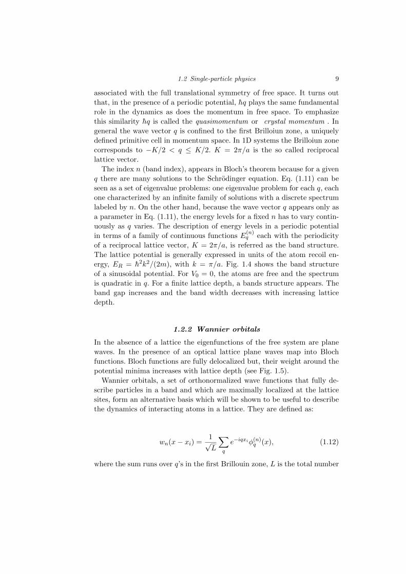
1.2.2 Wannier orbitals
In the absence of a lattice the eigenfunctions of the free system are plane
waves. In the presence of an optical lattice plane waves map into Bloch
functions. Bloch functions are fully delocalized but, their weight around the
potential minima increases with lattice depth (see Fig. 1.5).
Wannier orbitals, a set of orthonormalized wave functions that fully de-
scribe particles in a band and which are maximally localized at the lattice
sites, form an alternative basis which will be shown to be useful to describe
the dynamics of interacting atoms in a lattice. They are defined as:
wn(x− xi) =1√L
∑q
e−iqxiφ(n)q (x), (1.12)
where the sum runs over q’s in the first Brillouin zone, L is the total number
10 Ultracold atoms in optical lattices
Figure 1.5 Bloch functions in a periodic potential. Similar lattice depthsthan those ones of Fig.1.4
of lattice sites and xi is the position of the ith lattice site. In Fig. 1.6 we
show a Wannier orbital centered at the origin.
An intuitive picture of the form of a Wannier function can be gained if one
assumes the periodic function u(n)q (x) in equation 1.9 to be approximately
the same for all Bloch states in a band. Under this approximation
wn(x) ≈ u(n)(x)sin(kx)
kx, (1.13)
clearly showing that wn(x) looks likes u(n)(x) at the site center, but it
spreads out with gradually decreasing oscillations. The latter are needed
to ensure orthogonality.
1.2.3 Tight binding approximation
The tight-binding approximation deals with the case in which the overlap
between Wannier orbitals at different sites is enough to require corrections to
the picture of isolated particles but not too much as to render the picture of
localized wave functions completely irrelevant. In this regime, to a very good
approximation, one can only take into account overlap between Wannier
orbitals in nearest neighbor sites. Furthermore, if initially the atoms are
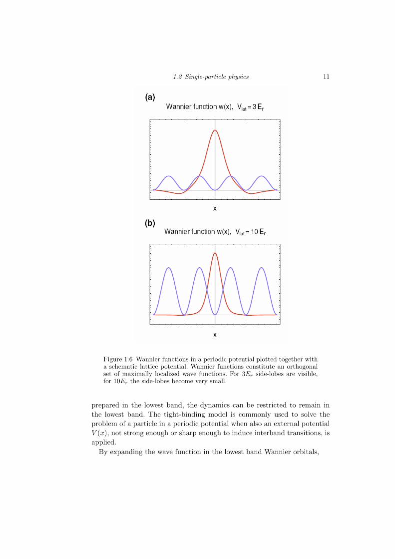
1.2 Single-particle physics 11
Figure 1.6 Wannier functions in a periodic potential plotted together witha schematic lattice potential. Wannier functions constitute an orthogonalset of maximally localized wave functions. For 3Er side-lobes are visible,for 10Er the side-lobes become very small.
prepared in the lowest band, the dynamics can be restricted to remain in
the lowest band. The tight-binding model is commonly used to solve the
problem of a particle in a periodic potential when also an external potential
V (x), not strong enough or sharp enough to induce interband transitions, is
applied.
By expanding the wave function in the lowest band Wannier orbitals,
12 Ultracold atoms in optical lattices
Ψ(x, t) =∑i
ψi(t)w0(x− xi), (1.14)
we get the following equations of motion
ih∂
∂tψi(t) = −J (ψi+1(t) + ψi−1(t)) + V (xi)ψi(t) + εoψi(t), (1.15)
with
J = −∫dxw∗0(xi)How0(x− xi+1)dx, (1.16)
εo =
∫dxw∗0(x)How0(x)dx (1.17)
J is the tunneling matrix element between nearest neighboring lattice sites
which decreases exponentially with lattice depth, and εo is the unperturbed
on site energy shift. Eq. (1.15) is known as the discrete Schrodinger equation
(DSE) or tight binding Schrodinger equation.
1.2.4 Semiclassical dynamics
Formalism
Solving Eq. (1.15) is presumably not possible for an arbitrary V (xi). How-
ever, one can get general insight to the nature of solutions by the application
of the correspondence principle. It is well known that wave-packet solutions
of the Schrodinger equation behave like classical particles obeying the equa-
tions of motion derived from the same classical Hamiltonian. The classical
Hamilton equations are
x =∂H
∂p, p = −∂H
∂x. (1.18)
Using the resemblance of the crystal momentum or quasimomentum to the
real momentum, the semiclassical equations of a wave packet in the first
band of a lattice can be written as [Ashcroft and Mermin (1976), Ziman
(1964)]:
x = v(0)(q) =1
h
dE(0)q
dq, hq = −dV (x)
dx. (1.19)
The semiclassical equations of motion describe how the position and wave
1.2 Single-particle physics 13
vector of a particle evolve in the presence of an external potential entirely
in terms of the band structure of the lattice. If we compare the acceleration
predicted by the model with the conventional newtonian equation, mx =
−dV (x)/dx, we can associate an effective mass induced by the presence of
the lattice,m∗. This is given by
1
m∗=
1
h2
d2
dq2E(0)q . (1.20)
If no external potential is applied, V (x) = 0, Bloch waves are the solutions
of tight binding equation: ψj(t) = f(q)j e−i(Eqt)/h , f
(q)j = 1√
Leiqaj with L is
the total number of lattice sites. If also periodic boundary conditions are
assumed, the quasimomentum q is restricted to be an integer multiple of2πLa . The lowest energy band dispersion relation in this case is given by
Eq = −2J cos(qa) (1.21)
From the above equation it is possible to see the connection between J and
the band width
J =(Eq=π
a− Eq=0
)/4 (1.22)
The effective mass becomes m∗ = h2
2Ja2 cos(qa)and close to the bottom of
the band q → 0, m∗ → h2
2Ja2. Since the tunneling decreases exponentially
with the lattice depth, the effective mass grows exponentially. In the pres-
ence of interactions, the large effective mass manifests itself in a substantial
enhancement of the interaction to kinetic energy ratio, in comparison to the
free particle case. This is the reason why atoms in optical lattices can easily
reach the strongly interaction regime. The strongly interacting regime cor-
responds to the regime in which the interaction energy of the atoms at a
given density dominates over their characteristic quantum kinetic energy.
References
Al Khawaja, U., Andersen, J. O., Proukakis, N. P., and Stoof, H. T. C. 2002. Lowdimensional Bose gases. Physical Review A, 66, 013615.
Altman, E., Demler, E., and Lukin, M. D. 2004. Probing many-body states ofultracold atoms via noise correlations. Phys. Rev. A, 70, 013603.
Ashcroft, N.W., and Mermin, N.D. 1976. Solid State Physics. Philadelphia: Saun-ders College.
Bakr, W. S., Peng, A., Tai, M. E., Ma, R., Simon, J., Gillen, J. I., Folling, S., Pollet,L., and Greiner, M. 2010. Probing the Superfluid-to-Mott Insulator Transitionat the Single-Atom Level. Science, 329, 547.
Blakie, P. B., and Porto, J. V. 2004. Adiabatic loading of bosons into opticallattices. Phys. Rev. A, 69, 013603.
Bloch, I., Dalibard, J., and Zwerger, W. 2008. Many-body physics with ultracoldgases. Rev. Mod. Phys., 80, 885.
Bogoliubov, N. N. 1947. On the theory of superfluidity. J. Phys. (USSR), 11, 23.Campbell, G. K., Mun, J., Boyd, M., Medley, P., Leanhardt, A. E., Marcassa, L. G.,
Pritchard, D. E., and Ketterle, W. 2006. Imaging the Mott insulator shells byusing atomic clock shifts. Science, 313, 649.
Castin, Y., and Dum, R. 1998. Low-temperature Bose-Einstein condensates in time-dependent traps: Beyond the U(1) symmetry-breaking approach. PhysicalReview A, 57, 3008–3021.
Chin, C., Grimm, R., Julienne, P., and Tiesinga, E. 2010. Feshbach resonances inultracold gases. Rev. Mod. Phys., 82, 1225.
Dalfovo, Franco, Giorgini, Stefano, Pitaevskii, Lev P., and Stringari, Sandro. 1999.Theory of Bose-Einstein condensation in trapped gases. Reviews of ModernPhysics, 71, 463–512.
Fisher, Matthew P. A., Weichman, Peter B., Grinstein, G., and Fisher, Daniel S.1989. Boson localization and the superfluid-insulator transition. PhysicalReview B, 40, 546–570.
Foelling, Simon, Widera, Artur, Muller, Torben, Gerbier, Fabrice, and Bloch, Im-manuel. 2006. Formation of Spatial Shell Structure in the Superfluid to MottInsulator Transition. Physical Review Letters, 97, 060403.
Gardiner, C. W. 1997. Particle-number-conserving Bogoliubov method whichdemonstrates the validity of the time-dependent Gross-Pitaevskii equation fora highly condensed Bose gas. Physical Review A, 56, 1414–1423.

References 15
Gemelke, Nathan, Zhang, Xibo, Hung, Chen-Lung, and Chin, Cheng. 2009. Insitu observation of incompressible Mott-insulating domains in ultracold atomicgases. Nature, 460, 995–998.
Gerbier, F., Widera, A., Folling, S., Mandel, O., Gericke, T., and Bloch, I. 2005a.Interference pattern and visibility of a Mott insulator. Physical Review A, 72.
Gerbier, F., Widera, A., Folling, S., Mandel, O., Gericke, T., and Bloch, I. 2005b.Phase coherence of an atomic Mott insulator. Physical Review Letters, 95.
Ginzburg, V. L., and Landau, L. D. 1950. On the theory of superconductivity. Zh.Eksp. Theor. Fiz., 20, 1064.
Greiner, Markus. 2003. PhD thesis: Ultracold quantum gases in three-dimensionaloptical lattice potentials. Dissertation in the Physics department of theLudwig-Maximilians-Universitat Munchen.
Hutchinson, D. A. W., Burnett, K., Dodd, R. J., Morgan, S. A., Rusch, M.,Zaremba, E., Proukakis, N. P., Edwards, M., and Clark, C. W. 2000. Gaplessmean-field theory of Bose-Einstein condensates. Journal of Physics B-AtomicMolecular and Optical Physics, 33, 3825–3846.
Jaksch, D., Bruder, C., Cirac, J. I., Gardiner, C. W., and Zoller, P. 1998. ColdBosonic Atoms in Optical Lattices. Phys. Rev. Lett., 81, 3108.
Jo, Gyu-Boong, Guzman, Jennie, Thomas, Claire K., Hosur, Pavan, Vishwanath,Ashvin, and Stamper-Kurn, Dan M. 2012. Ultracold Atoms in a TunableOptical Kagome Lattice. Physical Review Letters, 108, 045305.
Morgan, S. A. 2000. A gapless theory of Bose-Einstein condensation in dilute gasesat finite temperature. Journal of Physics B-Atomic Molecular and OpticalPhysics, 33, 3847–3893.
Mott, N. F. 1949. The basis of the electron theory of metals, with special referenceto the transition metals. Proceedings of the Physical Society of London SeriesA, 62, 416.
Penrose, O., and Onsage, L. 1956. Bose-Einstein Condensation and Liquid Helium.Phys. Rev., 104, 576.
Phillips, William D. 1998. Nobel Lecture: Laser cooling and trapping of neutralatoms. Reviews of Modern Physics, 70, 721–741.
Rey, A. M., Burnett, K., Roth, R., Edwards, M., Williams, C. J., and Clark, C. W.2003. Bogoliubov approach to superfluidity of atoms in an optical lattice.Journal of Physics B-Atomic Molecular and Optical Physics, 36, 825.
Sachdev, S. 2011. Quantum Phase Transitions. Cambridge University Press.Schellekens, M., Hoppeler, R., Perrin, A., Gomes, J. V., Boiron, D., Aspect, A., and
Westbrook, C. I. 2005. Hanbury Brown Twiss effect for ultracold quantumgases. Science, 310, 648–651.
Sebby-Strabley, J., Anderlini, M., Jessen, P. S., and Porto, J. V. 2006. Lattice ofdouble wells for manipulating pairs of cold atoms. Phys. Rev. A, 73, 033605.
Sherson, J. F., Weitenberg, C., Endres, M., Cheneau, M., Bloch, I., and Kuhr, S.2010. Single-atom-resolved fluorescence imaging of an atomic Mott insulator.Nature, 467, 68.
Soltan-Panahi, P., Struck, J., Hauke, P., Bick, A., Plenkers, W., Meineke, G.,Becker, C., Windpassinger, P., Lewenstein, M., and Sengstock, K. 2011. Multi-component quantum gases in spin-dependent hexagonal lattices. Nat Phys, 7,434–440.
Spielman, I. B., Phillips, W. D., and Porto, J. V. 2007. Mott-insulator transitionin a two-dimensional atomic Bose gas. Phys. Rev. Lett., 98, 080404.
16 References
Tarruell, Leticia, Greif, Daniel, Uehlinger, Thomas, Jotzu, Gregor, and Esslinger,Tilman. 2012. Creating, moving and merging Dirac points with a Fermi gasin a tunable honeycomb lattice. Nature, 483, 302–305.
Toth, E., Rey, A. M., and Blakie, P. B. 2008. Theory of correlations betweenultracold bosons released from an optical lattice. Phys. Rev. A, 78, 013627.
van Oosten, D., van der Straten, P., and Stoof, H. T. C. 2001. Quantum phases inan optical lattice. Physical Review A, 63, 053601.
Wirth, Georg, Olschlager, Matthias, and Hemmerich, Andreas. 2011. Evidence fororbital superfluidity in the P-band of a bipartite optical square lattice. NatPhys, 7, 147–153.
Ziman, J.M. 1964. Principles of the Theory of Solids. London, England: CambridgeUniversity Press.
2
Ultracold atoms in optical lattices
2.1 The Bose-Hubbard Hamiltonian
The simplest non trivial model that describes interacting bosons in a peri-
odic potential is the Bose-Hubbard Hamiltonian. This model has been used
to describe many different systems in solid state physics, such as short cor-
relation length superconductors, Josephson arrays, critical behavior of 4He
and, recently, cold atoms in optical lattices [Bloch et al. (2008)]. The Bose-
Hubbard Hamiltonian exhibits a quantum phase transition from a superfluid
to a Mott insulator state [Fisher et al. (1989)]. Its phase diagram has been
studied analytically and numerically with many different techniques and
confirmed experimentally using ultracold atomic systems in 1D, 2D and 3D
lattice geometries [Bloch et al. (2008)].
The Bose-Hubbard Hamiltonian can be derived from the second quantized
Hamiltonian that describes interacting bosonic atoms in an external trap-
ping potential plus lattice. In the grand canonical ensemble and assuming
the interactions are dominated by s-wave interactions (as it is the case for
in ultra cold gases) this Hamiltonian is given by [Jaksch et al. (1998)]:
H =
∫dxΨ†(x)
(− h2
2m∇2 + Vlat(x)
)Ψ(x) + (V (x)− µ)Ψ†(x)Ψ(x)
+2πash
2
m
∫dxΨ†(x)Ψ†(x)Ψ(x)Ψ(x), (2.1)
where Ψ†(x) is the bosonic field operator which creates an atom at the posi-
tion x, Vlatt(x) is the periodic lattice potential, V (x) denotes any additional
slowly- varying external potential that might be present (such as a harmonic
confinement used to collect the atoms), as is the scattering length ( the sin-
gle parameter which characterize the low energy collisions as explained in
18 Ultracold atoms in optical lattices
Chapter 3), and m the mass of an atom. µ is the chemical potential and
acts as a lagrange multiplier to fix the mean number of atoms in the grand
canonical ensemble.
Similar to the noninteracting situation where we used Wannier orbitals to
span the single particle wave function, it is convenient to expand the field
operator in terms of Wannier orbitals. Assuming that the vibrational energy
splitting between bands is the largest energy scale of the problem, atoms can
be loaded only in the lowest band, where they will reside under controlled
conditions. Then and one can restrict the basis to include only lowest band
Wannier orbitals w0(x),
Ψ(x) =∑j
ajw0(x− xj), (2.2)
Here aj is the annihilation operator at site j which obeys bosonic canonical
commutation relations (see Chapter 2). The sum is taken over the total
number of lattice sites. If Eq. (2.2) is inserted in H, and only tunneling
processes between nearest neighbor sites are kept and the interactions are
restricted to be onsite, one obtains the Bose-Hubbard Hamiltonian
HBH = −J∑〈j,i〉
a†i aj +1
2U∑j
a†j a†jajaj +
∑n
(Vj − µ)a†j aj . (2.3)
Here the notation 〈j, i〉 restricts the sum to nearest-neighbors sites. J is given
by Eq.(1.16) and
U =4πash
2
m
∫dx |w0(x)|4 , (2.4)
Vj = V (xj) (2.5)
The first term in the Hamiltonian proportional to J is a measure of the
kinetic energy of the system. Next-to-nearest neighbor tunneling amplitudes
are typically two orders of magnitude smaller than nearest-neighbor ones and
to a good approximation they can be neglected.
The second term of Eq.2.3 accounts for interatomic interactions. The pa-
rameter U measures the strength of the repulsion of two atoms at the same
lattice site. While J decreases exponentially with lattice depth V0, the U
increases as a power law, VD/4
0 , (D is the dimensionality of the lattice).
The third term in the Hamiltonian takes into account the energy offset
between lattice sites due to a slow varying external potential V (x).
2.1 The Bose-Hubbard Hamiltonian 19
2.1.1 The superfluid to Mott insulator transition
At zero temperature the physics described by the Bose-Hubbard Hamilto-
nian can be divided in two different regimes. The interaction dominated
regime when J is much smaller than U , and the atoms behave like an in-
sulator: the so-called Mott insulator [Mott (1949)], and the kinetic energy
dominated regime, when tunneling overwhelms the repulsion and the atoms
exhibit superfluid properties. The transition between the two regimes is a
consequence of the competition between the kinetic energy which tries to
delocalize the particles and the interaction energy which tries to localize
them and penalizes multiple-occupied lattice sites.
In the superfluid regime, the kinetic energy term dominates the Hamil-
tonian and the system behaves as a weakly interacting Bose gas. Quantum
fluctuations can be neglected and the system can be described by a macro-
scopic wave function. For a translationally invariant lattice the ground state
consists of all atoms in the 0-quasimomentum mode.
|ΨSF〉 =1√N !
(b†0
)N|0〉, (2.6)
where N is the total number of atoms and b†q = 1√L
∑j aje
iq·xj is the an-
nihilation operator of an atom with quasimomentum q and L is the total
number of lattice sites. Remember a is the lattice spacing.
Since the many body state is almost a product over identical single particle
wave functions, the system has a macroscopic well defined phase and large
number fluctuations ∼√N . The macroscopic occupation of a single mode
implies that the commutator of the annihilation and creation operators in
the condensate mode can be neglected with respect to the total number of
atoms in the mode. Therefore, to a good approximation the field operator
can be replaced by a c-number,
b0 → 〈b0〉 (2.7)
this approximation can be interpreted as giving to the field operator a non-
zero average, 〈b0〉 =√Neiθ, and thus a well defined phase to the system.
Because the original Hamiltonian is invariant under a global phase trans-
formation, the macroscopic occupation of a single mode can be linked to a
spontaneous symmetry breaking [Dalfovo et al. (1999)]. The wave function
associated with the condensate mode, in this case the zero quasi-momentum
eigenstate ψj =√
NL e
iθ, is often called “condensate wave function”. The
one particle density matrix ρ(1)i,j ≡ 〈a
†j ai〉 in this case develops off-diagonal
20 Ultracold atoms in optical lattices
long range order Ginzburg and Landau (1950), meaning that spatial cor-
relations remain finite even for very large separation between particles:
lim|i−j|→∞ ρ(1)i,j ∼ lim|i−j|→∞ ψ
∗i ψj → N/L. Strictly speaking, in finite size
systems with well defined number of particles, neither the concept of bro-
ken symmetry, nor the one of off-diagonal long range order can be applied
[Gardiner (1997)]. However, the condensate wave function can still be deter-
mined by diagonalization of the one particle density matrix. The eigenstate
with larger eigenvalue corresponds to the condensate wave function [Penrose
and Onsage (1956)].
With increasing interatomic interactions, the average kinetic energy re-
quired for an atom to hop from one site to the next becomes insufficient
to overcome the interaction energy cost. Atoms tend to get localize at indi-
vidual lattice sites and fluctuations of the atom number at a given lattice
site penalized. In this strongly interacting limit, if the number of atoms is
commensurate with the number of lattice sites, the ground state of the sys-
tem enters the Mott insulator phase, characterized by localized atomic wave
functions and a fixed number of atoms per site [Mott (1949)].
|ΨMI〉 =∏j
1√no!
(a†j)no |0〉, (2.8)
where no = N/L is the filling factor or mean number of particles per site.
We have assumed that the number of particles is commensurate with lattice
sites, i.e. that no is an integer.
The lowest lying excitations that conserve particle number are particle-
hole excitations (adding plus removing a particle from the system) which
cost energy. The Mott phase consequently is characterized by the existence
of an energy gap. The gap is determined by the energy necessary to create
one particle-hole pair.
2.1.2 The phase diagram
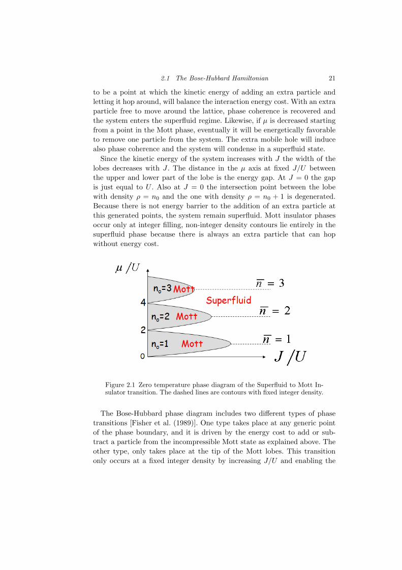
The zero temperature phase diagram [Fisher et al. (1989)] that describes the
Bose-Hubbard model in a translational invariant system (Vj = 0) exhibits
lobe-like Mott insulating phases in the J/U -µ plane, see Fig. 2.1. Each Mott
lobe is characterized by having a fixed integer density. Inside the lobes the
compressibility vanishes, ∂ρ/∂µ = 0, with ρ the density of the system.
The underlying physics of this phase diagram can be understood from
the following considerations. Imagine we start at some point in the Mott
insulating phase and increase µ while keeping J/U fixed. Then, there is going
2.1 The Bose-Hubbard Hamiltonian 21
to be a point at which the kinetic energy of adding an extra particle and
letting it hop around, will balance the interaction energy cost. With an extra
particle free to move around the lattice, phase coherence is recovered and
the system enters the superfluid regime. Likewise, if µ is decreased starting
from a point in the Mott phase, eventually it will be energetically favorable
to remove one particle from the system. The extra mobile hole will induce
also phase coherence and the system will condense in a superfluid state.
Since the kinetic energy of the system increases with J the width of the
lobes decreases with J . The distance in the µ axis at fixed J/U between
the upper and lower part of the lobe is the energy gap. At J = 0 the gap
is just equal to U . Also at J = 0 the intersection point between the lobe
with density ρ = n0 and the one with density ρ = n0 + 1 is degenerated.
Because there is not energy barrier to the addition of an extra particle at
this generated points, the system remain superfluid. Mott insulator phases
occur only at integer filling, non-integer density contours lie entirely in the
superfluid phase because there is always an extra particle that can hop
without energy cost.
Figure 2.1 Zero temperature phase diagram of the Superfluid to Mott In-sulator transition. The dashed lines are contours with fixed integer density.
The Bose-Hubbard phase diagram includes two different types of phase
transitions [Fisher et al. (1989)]. One type takes place at any generic point
of the phase boundary, and it is driven by the energy cost to add or sub-
tract a particle from the incompressible Mott state as explained above. The
other type, only takes place at the tip of the Mott lobes. This transition
only occurs at a fixed integer density by increasing J/U and enabling the
22 Ultracold atoms in optical lattices
bosons to overcome the on site repulsion. The two kinds of phase transitions
belong to different universality classes [Sachdev (2011)]. In the generic one,
the parameter equivalent to the reduced temperature, δ = T − Tc, which
describes finite temperature transitions is δ ∼ µ− µc, with µc the chemical
potential at the phase boundary. For the special fixed density on the other
hand one must take δ ∼ (J/U) − (J/U)c, with (J/U)c the critical value at
the tip the Mott lobes.
2.1.3 Decoupling mean field approximation
The Bose-Hubbard Hamiltonian is the simples model that describes inter-
acting bosons in a lattice, however an exact analytic treatment of its phase
diagram is not possible. Regardless of this difficulty, this Hamiltonian ad-
mits a simple approximated treatment, the so-called decoupling mean field
approximation [Fisher et al. (1989); van Oosten et al. (2001)], that captures
most of the features of the phase diagram discussed above. Here we present
a brief overview of the method. The decoupling mean field approximation is
carried out by introducing a real superfluid order parameter ψ = 〈a†j 〉 = 〈aj〉and then constructing a self-consistent mean-field theory. The kinetic energy
term is replaced by:
a†j ai → a†j〈ai〉+ 〈a†j〉ai − 〈a†j〉〈ai〉
= ψ(a†j + ai)− ψ2, (2.9)
when substituted into Eq. 2.3 yields
Hmean = −Jzψ∑j
(a†j + aj − ψ) +1
2U∑j
a†j a†jajaj +
∑j
(−µ)a†j aj ,(2.10)
Here z = 2D is the number of nearest-neighbor sites and L is the total
number of lattice sites. This Hamiltonian is local and the same for each
lattice site, therefore we will drop the subscript j in the following discussion.
By treating ψ as a small parameter, one can use perturbation theory
to calculate the mean field energy. Assuming commensurate filling N/L =
n0 = 1, 2, . . . , to zero order in ψ the ground state of the system will have
energy E(0)n0 and exactly n0 particles per site (Eq.3.37). In this unperturbed
occupation number basis the odd powers of the expansion of the energy in
ψ will always be zero. Up to four order, the ground state energy becomes
2.1 The Bose-Hubbard Hamiltonian 23
E = E(0) + ψ2E(2) + ψ4E(4) (2.11)
with E(2) =∑1
m=−1,m 6=0|〈n0|Jz(a+a†)|n0+m〉|2
E(0)n0−E(0)
n0+m
+ Jz. If we now minimize the
energy as a function of ψ, we find that ψ 6= 0 when E(2) < 0 and that ψ = 0
when E(2) > 0. This means that E(2) = 0 determines the boundary between
the superfluid and the insulator phases. The solution E(2) = 0 occurs for
[van Oosten et al. (2001)]
µ±
Jz=
1
2
U
Jz(2n0 − 1)− 1±
√(U
Jz
)2
− 2U
Jz(2n0 + 1) + 1
(2.12)
By equating µ+ = µ− one finds the critical value at the tip of each lobe:
(U
J
)c
= z(
2n0 + 1 +√
(2n0 + 1)2 − 1)
(2.13)
2.1.4 Bogoliubov treatment of the superfluid to Mott transition
An alternative systematic approach to deal with the weakly interacting
regime of the Bose-Hubbard model uses the ideas developed by N. Bogoli-
ubov in 1947 [Bogoliubov (1947)]. The Bogoliubov approximation treats the
field operator as a c-number plus a small fluctuating term. The c-number
describes the condensate or the coherent part of the bosonic matter field and
the fluctuating term accounts for quantum correlations. Since in a weakly
interacting gas quantum correlations are small, one can neglect third and
higher order terms in the fluctuating field and derive an effective quadratic
Hamiltonian which can be exactly diagonalized. In the following, we will
apply the Bogoliubov approximation to the Bose-Hubbard Hamiltonian and
derive the correspondent Bogoliubov-de Genes(BdG) equations as developed
in Refs. [van Oosten et al. (2001); Rey et al. (2003)]. We will restrict our
analysis to T = 0.
The Bogoliubov approximation
In the very weakly interacting regime, to a good approximation, the field
operator can be written in terms of a c-number plus a fluctuation operator:
aj = ψj + ϕj . (2.14)
24 Ultracold atoms in optical lattices
Replacing this expression for aj in the Bose-Hubbard Hamiltonian leads
to :
H = Eo + H1 + H2 + H3 + H4, (2.15)
with
H0 = −J∑〈i,j〉
ψ∗i ψj +∑i
(Vi − µ)|ψi|2 +U
2|ψi|4, (2.16)
H1 = −J∑〈i,j〉
ϕiψ∗j +
∑i
(Vi − µ+ U |ψi|2
)ψ∗i ϕi + h.c., (2.17)
H2 = −J∑〈i,j〉
ϕ†i ϕj +∑i
(Vi − µ)ϕ†i ϕi +
U
2
∑i
(ϕ2†i ψ
2i + ϕ2
iψ2∗i + (ϕ†i ϕi + ϕiϕ
†i )|ψi|
2), (2.18)
H3 = U∑i
ϕ†i ϕ†i ϕiψi + h.c., (2.19)
H4 =U
2
∑i
ϕ†i ϕ†i ϕiϕi, (2.20)
where 〈i, j〉 restricts the sum over nearest neighbors and h.c. stands for
the hermitian adjoint. The terms of the Hamiltonian have been grouped in
equations according to the number of non-condensate operators which they
contain.
The first step is the minimization of the energy functional H0. This re-
quires the condensate amplitudes ψi to be a solution of the following non-
linear equation,
µψi = −J∑〈i,j〉
ψj + (Vi + U |ψi|2)ψi (2.21)
This equation is known as the discrete nonlinear Schrodinger equation (DNLSE).
It is a discrete version of the Gross-Pitaevskii equation (GPE) (See Chapter
3). It can be also obtained by expanding the GPE equation in a Wannier
orbital basis and then using the tight binding approximation (see Sec1.15).
When ψi is a solution of Eq.2.21 the linear Hamiltonian H1 vanishes.
The quadratic Hamiltonian H2 accounts for the leading order corrections
to the DNLSE due to quantum fluctuations. The basis that diagonalizes
H2 defines the so -called quasiparticle states. Mathematically the diagonal-
ization procedure involves a linear canonical transformation of the single-
particle creation and annihilation operators a†i and ai into quasiparticle op-
2.1 The Bose-Hubbard Hamiltonian 25
erators α†s,αs. This transformation is what is known as Bogoliubov transfor-
mation and is given by
ϕi =∑s6=0
usi αs − v∗si α†s. (2.22)
In general the spectrum of fluctuations includes a zero mode s = 0. This
mode is the Goldstone boson associated with the breaking of global phase
invariance by the condensate. The zero mode is essentially non-perturbative
and it introduces an artificial infrared divergence in low dimensional models.
For this reason quadratic approximations are actually improved if the con-
tribution from this mode is neglected all together [Al Khawaja et al. (2002)].
A different way to deal with the zero mode has been proposed by Castin
and Dum (1998); Gardiner (1997); Hutchinson et al. (2000); Morgan (2000).
For simplicity we are going to ignore zero mode fluctuations and restrict the
fluctuation operators to act only on the excited states.
The Bogoliubov transformation Eq. 2.22 is required to be canonical. By
canonical it is meant that it preserves the commutation relations and leads to
bosonic quasiparticles. To satisfy it, the amplitudes usi , vsi are constrained
by the conditions: ∑i
u∗si us′i − v∗si vs′i = δss′, (2.23)∑
i
usivs′i − v∗si u∗s′i = 0. (2.24)
The necessary and sufficient conditions that the quasiparticle amplitudes
have to fulfill to diagonalize the Hamiltonian are provided by the so called
Bogoliubov-de Gennes (BdG) equations(L MM∗ L
)(us
vs
)= ωBs
(us
−vs
)(2.25)
with us = (us1, us2 . . . u
sL) , vs = (vs1, v
s2 . . . v
sL) and ψ = (ψ1, ψ2 . . . ψL). The
matrices L and M are given by
Lij = −Jf(i, j) + δij(2U |ψi|2 + Vi − µ) (2.26)
Mij = −Uψ2i δij . (2.27)
with δij the Kronecker delta which is one if i = j and zero otherwise and
f(i, j) a function which is equal to one if the sites i and j are nearest-
neighbors and zero otherwise. If the BdG equations are satisfied, the quadratic
Hamiltonian, up to constant terms, takes the form
26 Ultracold atoms in optical lattices
H2 =∑s6=0
ωBs α†sαs. (2.28)
The quasi-particle energies ωBs come in pairs: if ωBs is a solution for the
amplitudes (us,vs) then −ωBs is also a solution for the amplitudes (vs∗,us∗).
The solution with zero energy is always a solution and in this case the
amplitudes must be proportional to the condensate (v0,u0) ∝ (ψ,ψ). We
explicitly exclude the zero mode solution to guarantee that the excitations
are orthogonal to the condensate.
In a zero temperature gas the fraction of atoms which are not part of the
condensate is generally referred to as the quantum depletion, ρd, Under the
Bogoliubov approximation, the quantum depletion is given by
ρd =∑j
⟨ϕ†jϕj
⟩=∑j,s6=0
|vsj |2 (2.29)
N =∑j
|ψj |2 + ρd (2.30)
Translationally invariant system
To understand the physics captured by the Bogoliubov approximation, we
study the case where no external confinement is present, Vj = 0. We assume a
D dimensional separable square optical lattice with equal tunneling matrix
element J in all directions and periodic boundary conditions. The total
number of sites is again L.
Due to the translational symmetry of the system the condensate ampli-
tudes are constant over the lattice, ψj =√nc. The quasiparticle modes have
a plane wave character and therefore can be related to quasimomentum
modes:
uqj =1√Leiq·xjuq, vqj =
1√Leiq·xjvq. (2.31)
Here the vector q = q1, q2, . . . qd denotes the quasi-momentum, whose
components assume discrete values which are integer multiples of 2π
a D√L
. a
is the lattice spacing. The amplitudes uq and vq must satisfy the condition
|uq|2− |vq|2 = 1 and can all be chosen to be real and to depend only on the
modulus of the wave vector (uq = u−q, vq = v−q).
In the translationally invariant system the DNLSE reduces to
µ = −zJ + ncU (2.32)
where z is the number of nearest neighbors z = 2D.
2.1 The Bose-Hubbard Hamiltonian 27
The BdG equations become the following 2× 2 eigenvalue problem(Lqq −Mq−qMq−q −Lqq
)(uqvq
)= ωq
(uqvq
), (2.33)
with
Lqq = εq + ncU, Mq−q = ncU. (2.34)
Here we have introduced the definition εq = 4J∑D
i=1 sin2( qia2 ).
The quasiparticle energies ωq and modes are found by diagonalizing Eq.(2.34):
ω2q = L2
qq −M2q−q = εq
2 + 2Uncεq, (2.35)
u2q =Lqq + ωq
2ωq=εq + ncU + ωq
2ωq, (2.36)
v2q =Lqq − ωq
2ωq=εq + ncU − ωq
2ωq, (2.37)
uqvq = −Mq−q2ωq
=ncU
2ωq(2.38)
and
n = nc +1
L
∑q 6=0
v2q, (2.39)
with n the total density, n = N/L. The constrain that fixes the number of
particles can be written as
nc = n− 1
L
∑q 6=0
(εq + Unc
2ωq− 1
2
). (2.40)
Note that, as opposed to the free particle system where for high momentum
always the single particle energy (which grows as q2) is dominant, in the
presence of the lattice the single particle excitations are always bounded by
4JD, when the atoms are restricted to populate the first band. Therefore, in
the regime Unc/J > 1 the interaction term dominates for all quasimomen-
tum and so ωq ∼√
2Uncεq. Thus, to a good approximation the condensate
fraction can be written as:
nc ≈ g −√UncJ
α (2.41)
28 Ultracold atoms in optical lattices
with
α = α(D,L) ≡ 1
L
∑q 6=0
√J
2√
2εq(2.42)
g = n+L− 1
2L(2.43)
α is a dimensionless quantity which depends only on the dimensionality of
the system and L. Because Eqs. ((2.35)-(2.36)) are completely determined if
nc is known, by solving Eq. (2.41) we obtain all necessary information. The
solution of the algebraic equation is:
nc ≈ g +α2U
2J−√gα2U
J+α4U2
4J2. (2.44)
Eq. (2.44) tells us that in the strongly interacting regime the condensate frac-
tion decreases with increasing U/J but it only vanishes when U/J → ∞.
The BdG equations therefore fail to predict any superfluid to Mott insu-
lator phase transition. Since for non-integer fillings the system is never a
Mott insulator, the BdG equations describe much better the incommensu-
rate regime.
2.1.5 External trapping potential
Up to this point we have discussed the basic aspects of the superfluid-Mott
insulator transition in a translationally invariant system. The situation is
different for a inhomogeneous system with a fixed total number of atoms
and external confinement. This is the case realized in experiments, where
besides the lattice there is a harmonic trap that collects the atoms at the
center. In this case, the density of atoms is not fixed since the atoms can
redistribute over the lattice and change the local filling factor.
To deal with the inhomogeneous case, it is possible to define an effective
local chemical potential, µj = µ−Vj, at each lattice site j. If the change in the
mean number of atoms between neighboring sites is small, the system can be
treated locally as an homogeneous system. Because in the inhomogeneous
case, the local chemical potential is fixed by the density, as the ratio U/J is
changed the system can cross locally the boundary between the superfluid
and Mott insulator phases. For example if the chemical potential at the
trap center falls into the n0 = 2 Mott lobe, one obtains a series of Mott
domains separated by a superfluid as one moves from the enter to the edge
2.1 The Bose-Hubbard Hamiltonian 29
of the cloud. In this manner, all different phases that exist for given J/U
are present simultaneously.
The existence of such “wedding-cake-like” density profiles in the Mott in-
sulator regime is supported by Monte Carlo calculations in one, two, and
three dimensions [Bloch et al. (2008)]. The shell structure has been ex-
perimentally measured by using indirect methods such as mean field shifts
[Campbell et al. (2006)] and spatially selective microwave transitions to-
gether with spin changing collisions [Foelling et al. (2006)]. Just recently
direct in-situ imaging methods with single lattice site resolution have suc-
cessfully resolved the shell structure in 2D systems [Gemelke et al. (2009);
Bakr et al. (2010); Sherson et al. (2010)].

References
Al Khawaja, U., Andersen, J. O., Proukakis, N. P., and Stoof, H. T. C. 2002. Lowdimensional Bose gases. Physical Review A, 66, 013615.
Altman, E., Demler, E., and Lukin, M. D. 2004. Probing many-body states ofultracold atoms via noise correlations. Phys. Rev. A, 70, 013603.
Ashcroft, N.W., and Mermin, N.D. 1976. Solid State Physics. Philadelphia: Saun-ders College.
Bakr, W. S., Peng, A., Tai, M. E., Ma, R., Simon, J., Gillen, J. I., Folling, S., Pollet,L., and Greiner, M. 2010. Probing the Superfluid-to-Mott Insulator Transitionat the Single-Atom Level. Science, 329, 547.
Blakie, P. B., and Porto, J. V. 2004. Adiabatic loading of bosons into opticallattices. Phys. Rev. A, 69, 013603.
Bloch, I., Dalibard, J., and Zwerger, W. 2008. Many-body physics with ultracoldgases. Rev. Mod. Phys., 80, 885.
Bogoliubov, N. N. 1947. On the theory of superfluidity. J. Phys. (USSR), 11, 23.Campbell, G. K., Mun, J., Boyd, M., Medley, P., Leanhardt, A. E., Marcassa, L. G.,
Pritchard, D. E., and Ketterle, W. 2006. Imaging the Mott insulator shells byusing atomic clock shifts. Science, 313, 649.
Castin, Y., and Dum, R. 1998. Low-temperature Bose-Einstein condensates in time-dependent traps: Beyond the U(1) symmetry-breaking approach. PhysicalReview A, 57, 3008–3021.
Chin, C., Grimm, R., Julienne, P., and Tiesinga, E. 2010. Feshbach resonances inultracold gases. Rev. Mod. Phys., 82, 1225.
Dalfovo, Franco, Giorgini, Stefano, Pitaevskii, Lev P., and Stringari, Sandro. 1999.Theory of Bose-Einstein condensation in trapped gases. Reviews of ModernPhysics, 71, 463–512.
Fisher, Matthew P. A., Weichman, Peter B., Grinstein, G., and Fisher, Daniel S.1989. Boson localization and the superfluid-insulator transition. PhysicalReview B, 40, 546–570.
Foelling, Simon, Widera, Artur, Muller, Torben, Gerbier, Fabrice, and Bloch, Im-manuel. 2006. Formation of Spatial Shell Structure in the Superfluid to MottInsulator Transition. Physical Review Letters, 97, 060403.
Gardiner, C. W. 1997. Particle-number-conserving Bogoliubov method whichdemonstrates the validity of the time-dependent Gross-Pitaevskii equation fora highly condensed Bose gas. Physical Review A, 56, 1414–1423.
References 31
Gemelke, Nathan, Zhang, Xibo, Hung, Chen-Lung, and Chin, Cheng. 2009. Insitu observation of incompressible Mott-insulating domains in ultracold atomicgases. Nature, 460, 995–998.
Gerbier, F., Widera, A., Folling, S., Mandel, O., Gericke, T., and Bloch, I. 2005a.Interference pattern and visibility of a Mott insulator. Physical Review A, 72.
Gerbier, F., Widera, A., Folling, S., Mandel, O., Gericke, T., and Bloch, I. 2005b.Phase coherence of an atomic Mott insulator. Physical Review Letters, 95.
Ginzburg, V. L., and Landau, L. D. 1950. On the theory of superconductivity. Zh.Eksp. Theor. Fiz., 20, 1064.
Greiner, Markus. 2003. PhD thesis: Ultracold quantum gases in three-dimensionaloptical lattice potentials. Dissertation in the Physics department of theLudwig-Maximilians-Universitat Munchen.
Hutchinson, D. A. W., Burnett, K., Dodd, R. J., Morgan, S. A., Rusch, M.,Zaremba, E., Proukakis, N. P., Edwards, M., and Clark, C. W. 2000. Gaplessmean-field theory of Bose-Einstein condensates. Journal of Physics B-AtomicMolecular and Optical Physics, 33, 3825–3846.
Jaksch, D., Bruder, C., Cirac, J. I., Gardiner, C. W., and Zoller, P. 1998. ColdBosonic Atoms in Optical Lattices. Phys. Rev. Lett., 81, 3108.
Jo, Gyu-Boong, Guzman, Jennie, Thomas, Claire K., Hosur, Pavan, Vishwanath,Ashvin, and Stamper-Kurn, Dan M. 2012. Ultracold Atoms in a TunableOptical Kagome Lattice. Physical Review Letters, 108, 045305.
Morgan, S. A. 2000. A gapless theory of Bose-Einstein condensation in dilute gasesat finite temperature. Journal of Physics B-Atomic Molecular and OpticalPhysics, 33, 3847–3893.
Mott, N. F. 1949. The basis of the electron theory of metals, with special referenceto the transition metals. Proceedings of the Physical Society of London SeriesA, 62, 416.
Penrose, O., and Onsage, L. 1956. Bose-Einstein Condensation and Liquid Helium.Phys. Rev., 104, 576.
Phillips, William D. 1998. Nobel Lecture: Laser cooling and trapping of neutralatoms. Reviews of Modern Physics, 70, 721–741.
Rey, A. M., Burnett, K., Roth, R., Edwards, M., Williams, C. J., and Clark, C. W.2003. Bogoliubov approach to superfluidity of atoms in an optical lattice.Journal of Physics B-Atomic Molecular and Optical Physics, 36, 825.
Sachdev, S. 2011. Quantum Phase Transitions. Cambridge University Press.Schellekens, M., Hoppeler, R., Perrin, A., Gomes, J. V., Boiron, D., Aspect, A., and
Westbrook, C. I. 2005. Hanbury Brown Twiss effect for ultracold quantumgases. Science, 310, 648–651.
Sebby-Strabley, J., Anderlini, M., Jessen, P. S., and Porto, J. V. 2006. Lattice ofdouble wells for manipulating pairs of cold atoms. Phys. Rev. A, 73, 033605.
Sherson, J. F., Weitenberg, C., Endres, M., Cheneau, M., Bloch, I., and Kuhr, S.2010. Single-atom-resolved fluorescence imaging of an atomic Mott insulator.Nature, 467, 68.
Soltan-Panahi, P., Struck, J., Hauke, P., Bick, A., Plenkers, W., Meineke, G.,Becker, C., Windpassinger, P., Lewenstein, M., and Sengstock, K. 2011. Multi-component quantum gases in spin-dependent hexagonal lattices. Nat Phys, 7,434–440.
Spielman, I. B., Phillips, W. D., and Porto, J. V. 2007. Mott-insulator transitionin a two-dimensional atomic Bose gas. Phys. Rev. Lett., 98, 080404.

32 References
Tarruell, Leticia, Greif, Daniel, Uehlinger, Thomas, Jotzu, Gregor, and Esslinger,Tilman. 2012. Creating, moving and merging Dirac points with a Fermi gasin a tunable honeycomb lattice. Nature, 483, 302–305.
Toth, E., Rey, A. M., and Blakie, P. B. 2008. Theory of correlations betweenultracold bosons released from an optical lattice. Phys. Rev. A, 78, 013627.
van Oosten, D., van der Straten, P., and Stoof, H. T. C. 2001. Quantum phases inan optical lattice. Physical Review A, 63, 053601.
Wirth, Georg, Olschlager, Matthias, and Hemmerich, Andreas. 2011. Evidence fororbital superfluidity in the P-band of a bipartite optical square lattice. NatPhys, 7, 147–153.
Ziman, J.M. 1964. Principles of the Theory of Solids. London, England: CambridgeUniversity Press.
![Workshop on Quantum Simulations with Ultracold Atomspeople.sissa.it/~andreatr/WORKSHOP_QUANTUM_SIMULATIONS...synthetic gauge potentials for cold atoms in optical lattices [1,2,3]](https://img.pdfslide.us/doc/110x75/60dd079a657564360213b425/workshop-on-quantum-simulations-with-ultracold-andreatrworkshopquantumsimulations.jpg)