Embed Size (px)
Citation preview
1
Transportation problem
The transportation problem seeks the determination of a minimum cost transportation plan for a single commodity from a number of sources to a number of destinations.
It requires the specification of the level of supply at each source, the amount of demand at each destination, and the transportation cost from each source to each destination.
The transportation problem is linear if the cost on a route is directly proportional to the amount transported; otherwise it is nonlinear.
2
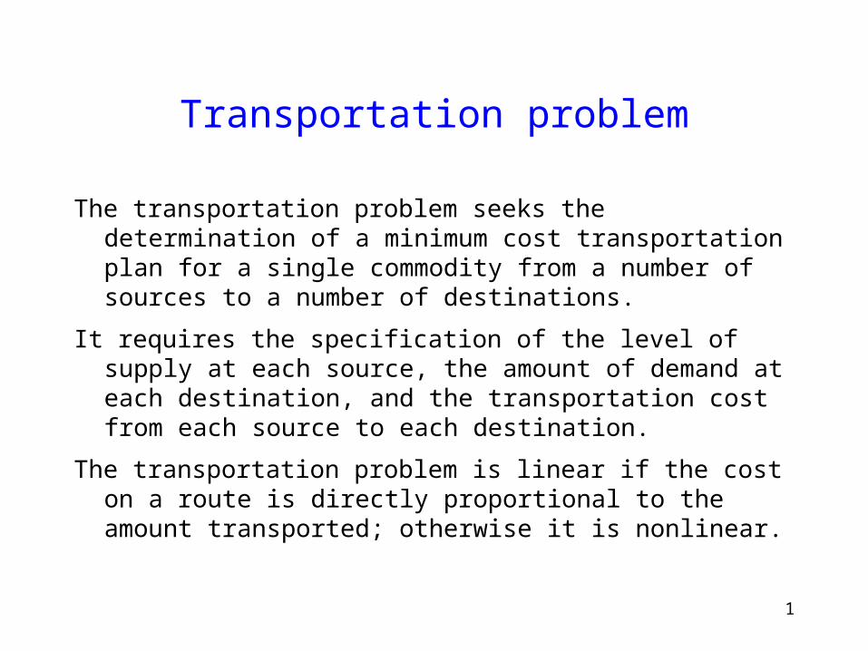
Assume there are n sources and k destinations. The amount of supply at source i is sour(i) and the demand at destination j is dest(j). The unit transportation cost between source i and destination j is cost(i,j). If x(i,j) is the amount transported from source i to destination j then the transportation problem is given as
min i,jf(i,j)
s.t. jx(i,j)sour(i) i=1,2,,n
ix(i,j)dest(j) j=1,2,,k
x(i,j)0 i=1,2,,n and j=1,2,,kIf f(i,j)=cost(i,j)*x(i,j) for all i and j, the problem is linear.
3
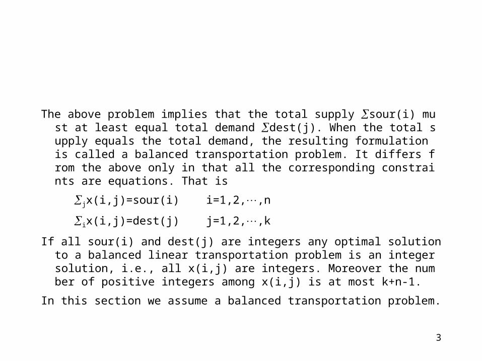
The above problem implies that the total supply sour(i) must at least equal total demand dest(j). When the total supply equals the total demand, the resulting formulation is called a balanced transportation problem. It differs from the above only in that all the corresponding constraints are equations. That is
jx(i,j)=sour(i) i=1,2,,n
ix(i,j)=dest(j) j=1,2,,k
If all sour(i) and dest(j) are integers any optimal solution to a balanced linear transportation problem is an integer solution, i.e., all x(i,j) are integers. Moreover the number of positive integers among x(i,j) is at most k+n-1.
In this section we assume a balanced transportation problem.
4
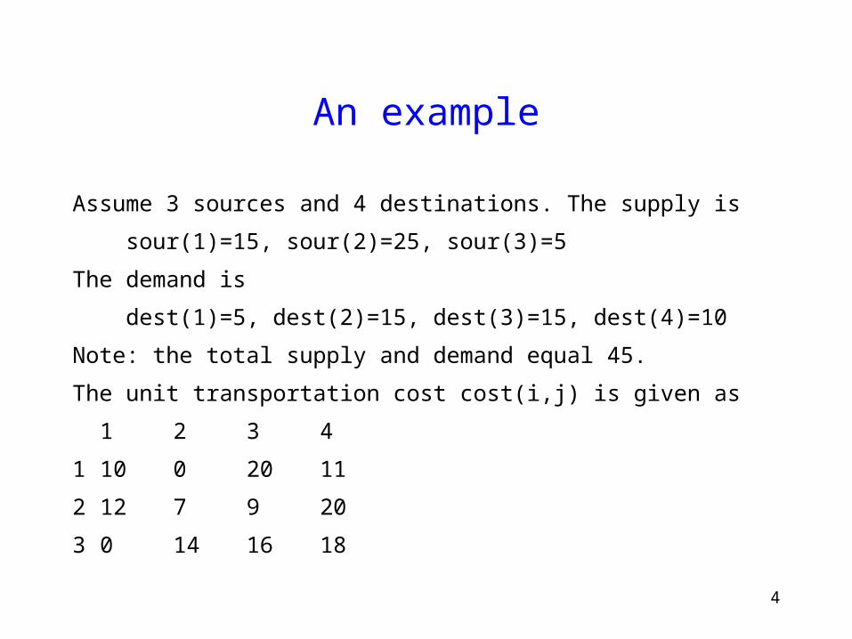
An example
Assume 3 sources and 4 destinations. The supply is sour(1)=15, sour(2)=25, sour(3)=5The demand is dest(1)=5, dest(2)=15, dest(3)=15, dest(4)=10Note: the total supply and demand equal 45.The unit transportation cost cost(i,j) is given as 1 2 3 41 10 0 20 112 12 7 9 203 0 14 16 18
5
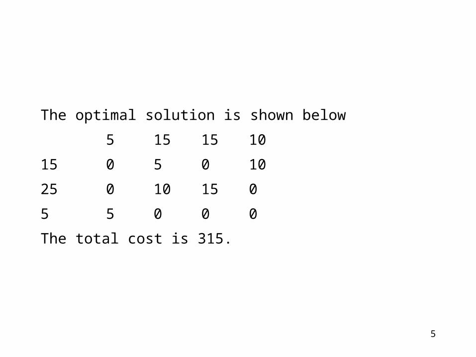
The optimal solution is shown below
5 15 15 10
15 0 5 0 10
25 0 10 15 0
5 5 0 0 0
The total cost is 315.
6
Classical genetic algorithms
A straightforward approach in defining the chromosome for a solution in the transportation problem is to create a vector (v(1),,v(p)) where p=nk. Each component v(i) represents an integer associated with row j and column m in the allocation matrix, where j=(i-1)/k+1 and m=(i-1) mod k+1.
7
Constraint satisfaction
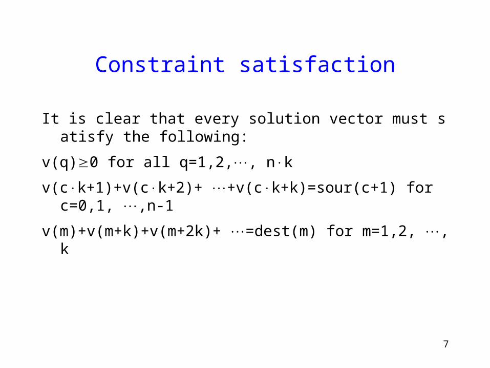
It is clear that every solution vector must satisfy the following:
v(q)0 for all q=1,2,, nkv(ck+1)+v(ck+2)+ +v(ck+k)=sour(c+1) for c=0,1, ,n-1v(m)+v(m+k)+v(m+2k)+ =dest(m) for m=1,2, ,k
8
Evaluation function
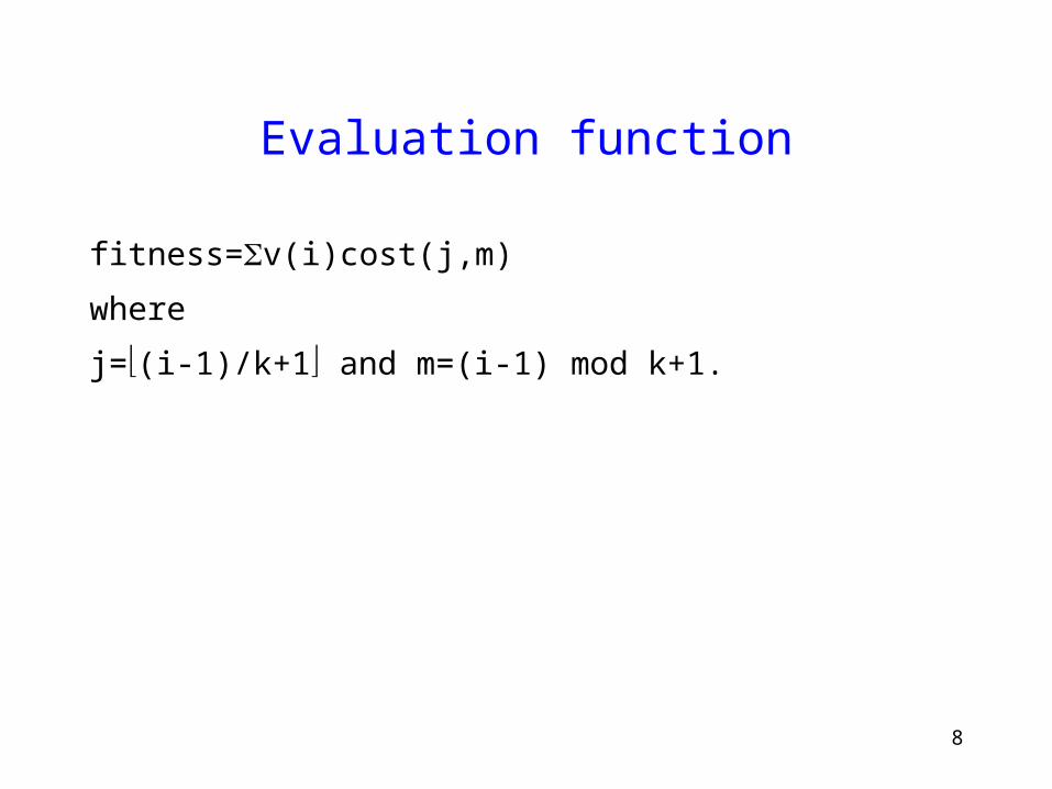
fitness=v(i)cost(j,m)
where
j=(i-1)/k+1 and m=(i-1) mod k+1.
9
Genetic operators
There is no natural definition of genetic operators the transportation problem with the above representation.
Mutation is usually defined as a change in a single gene in a solution vector. This, for our problems, would trigger a series of changes in different places (at least three other changes) in order to maintain the constraint equalities.
The situation is even worse if we try to define a crossover operator.
Conclusion: the above vector representation is not the most suitable for defining genetic operators in our problems.
10
Incorporating problem-specific knowledge
Can we improve the representation of a solution while preserving the basic structure of this vector representation?
The answer is yes, but we have to incorporate problem-specific knowledge into the representation.
11
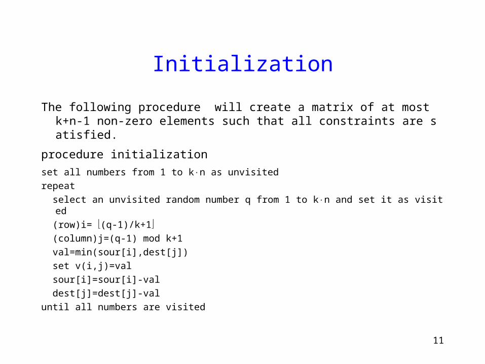
Initialization
The following procedure will create a matrix of at most k+n-1 non-zero elements such that all constraints are satisfied.
procedure initializationset all numbers from 1 to kn as unvisitedrepeat select an unvisited random number q from 1 to kn and set it as visited (row)i= (q-1)/k+1 (column)j=(q-1) mod k+1 val=min(sour[i],dest[j]) set v(i,j)=val sour[i]=sour[i]-val dest[j]=dest[j]-valuntil all numbers are visited
12
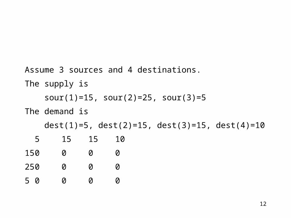
Assume 3 sources and 4 destinations. The supply is sour(1)=15, sour(2)=25, sour(3)=5The demand is dest(1)=5, dest(2)=15, dest(3)=15, dest(4)=10
5 15 15 1015 0 0 0 025 0 0 0 05 0 0 0 0
13
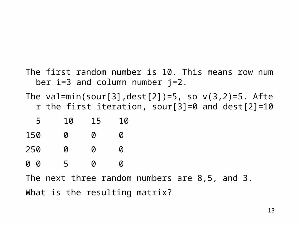
The first random number is 10. This means row number i=3 and column number j=2.
The val=min(sour[3],dest[2])=5, so v(3,2)=5. After the first iteration, sour[3]=0 and dest[2]=10
5 10 15 1015 0 0 0 025 0 0 0 00 0 5 0 0The next three random numbers are 8,5, and 3.What is the resulting matrix?

14
5 10 15 1015 0 0 0 025 0 0 0 00 0 5 0 0The random numbers is 8 (corresponding to row 2 and column
4).5 10 15 0
15 0 0 0 015 0 0 0 100 0 5 0 0
15
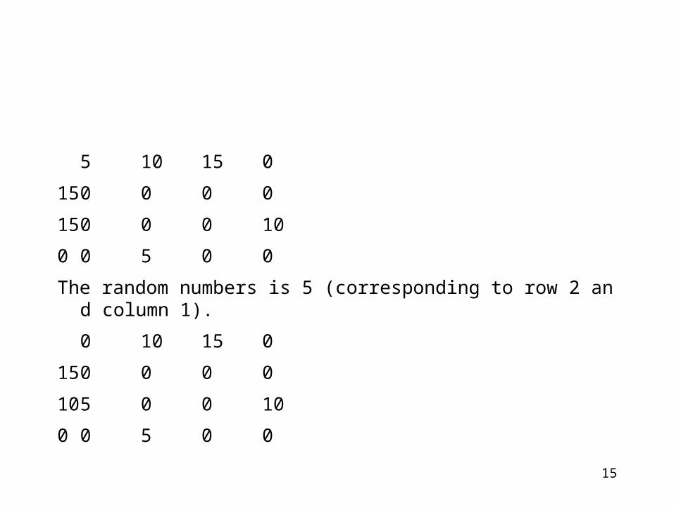
5 10 15 015 0 0 0 015 0 0 0 100 0 5 0 0The random numbers is 5 (corresponding to row 2 and column
1).0 10 15 0
15 0 0 0 010 5 0 0 100 0 5 0 0
16
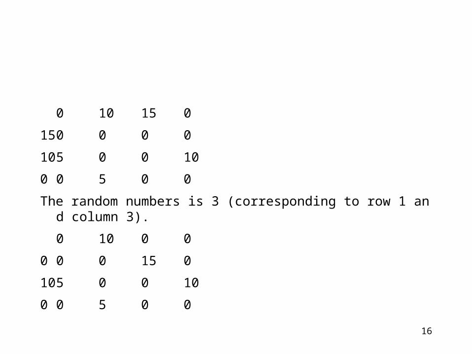
0 10 15 015 0 0 0 010 5 0 0 100 0 5 0 0The random numbers is 3 (corresponding to row 1 and column
3).0 10 0 0
0 0 0 15 010 5 0 0 100 0 5 0 0
17
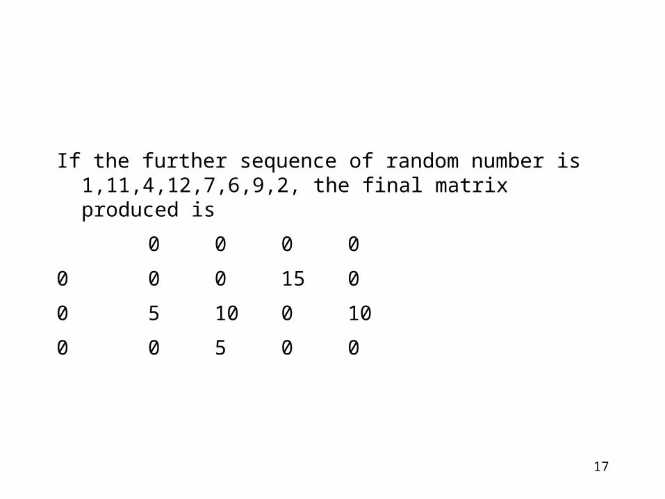
If the further sequence of random number is 1,11,4,12,7,6,9,2, the final matrix produced is
0 0 0 0
0 0 0 15 0
0 5 10 0 10
0 0 5 0 0
18
This technique can generate any feasible solution that contains at most k+n-1 non-zero integer elements.
It will not generate other solutions which, though feasible, do not share this characteristic.
The initialization procedure would certainly have to be modified when we attempt to solve non-linear versions of the transportation problems.
19
The knowledge of the problem and its solution characteristic gives us an opportunity to represent a solution to the transportation problem as a vector.
A solution vector will be a sequence of nk distinct integers from the range <1, nk>, which (according to the procedure initialization) would produce an acceptable solution.
In other words we would view a solution-vector as a permutation of numbers, and we would look for particular permutations which correspond to the optimal solution.
20
Constraint satisfaction
Any permutation of kn distinct numbers produces a unique solution which satisfies all constraints. This is guaranteed by procedure initialization.
21
Evaluation function
This is relatively easy. Any permutation would correspond to a unique matrix <v(i,j)>.
The evaluation function is i,jv(i,j)cost(i,j)
22
Genetic operators
Inversion: any solution vector (x(1),x(2),, x(q)) (q=kn) can be easily inverted into another solution vector (x(q), x(q-1), , x(1))
Swap: any two elements of a solution vector, say x(i) and x(j) can be swapped easily resulting in another solution vector.
Crossover: PMX, CX, OX
23
A matrix as representation structure
Perhaps the most natural representation of a solution for the transportation problem is a two dimensional structure. After all, this is how the problem is presented and solved by hand. In other words, a matrix V=(v(i,j)) (1ik, 1jn) may represent a solution.
24
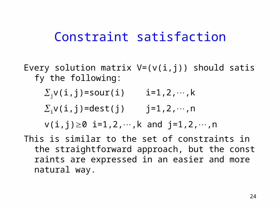
Constraint satisfaction
Every solution matrix V=(v(i,j)) should satisfy the following: jv(i,j)=sour(i) i=1,2,,k
iv(i,j)=dest(j) j=1,2,,n
v(i,j)0 i=1,2,,k and j=1,2,,nThis is similar to the set of constraints in the straightforwa
rd approach, but the constraints are expressed in an easier and more natural way.
25
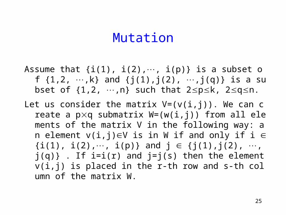
Mutation
Assume that {i(1), i(2),, i(p)} is a subset of {1,2, ,k} and {j(1),j(2), ,j(q)} is a subset of {1,2, ,n} such that 2pk, 2qn.
Let us consider the matrix V=(v(i,j)). We can create a pq submatrix W=(w(i,j)) from all elements of the matrix V in the following way: an element v(i,j)V is in W if and only if i {i(1), i(2),, i(p)} and j {j(1),j(2), ,j(q)} . If i=i(r) and j=j(s) then the element v(i,j) is placed in the r-th row and s-th column of the matrix W.
26
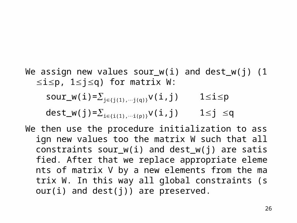
We assign new values sour_w(i) and dest_w(j) (1ip, 1jq) for matrix W:
sour_w(i)=j{j(1),j(q)}v(i,j) 1ip
dest_w(j)=i{i(1),i(p)}v(i,j) 1j q
We then use the procedure initialization to assign new values too the matrix W such that all constraints sour_w(i) and dest_w(j) are satisfied. After that we replace appropriate elements of matrix V by a new elements from the matrix W. In this way all global constraints (sour(i) and dest(j)) are preserved.
27
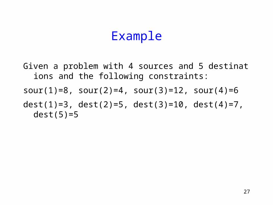
Example
Given a problem with 4 sources and 5 destinations and the following constraints:
sour(1)=8, sour(2)=4, sour(3)=12, sour(4)=6dest(1)=3, dest(2)=5, dest(3)=10, dest(4)=7, dest(5)=5

28
The following matrix V is selected as a parent for mutation
0 0 5 0 3
0 4 0 0 0
0 0 5 7 0
3 1 0 0 2
29
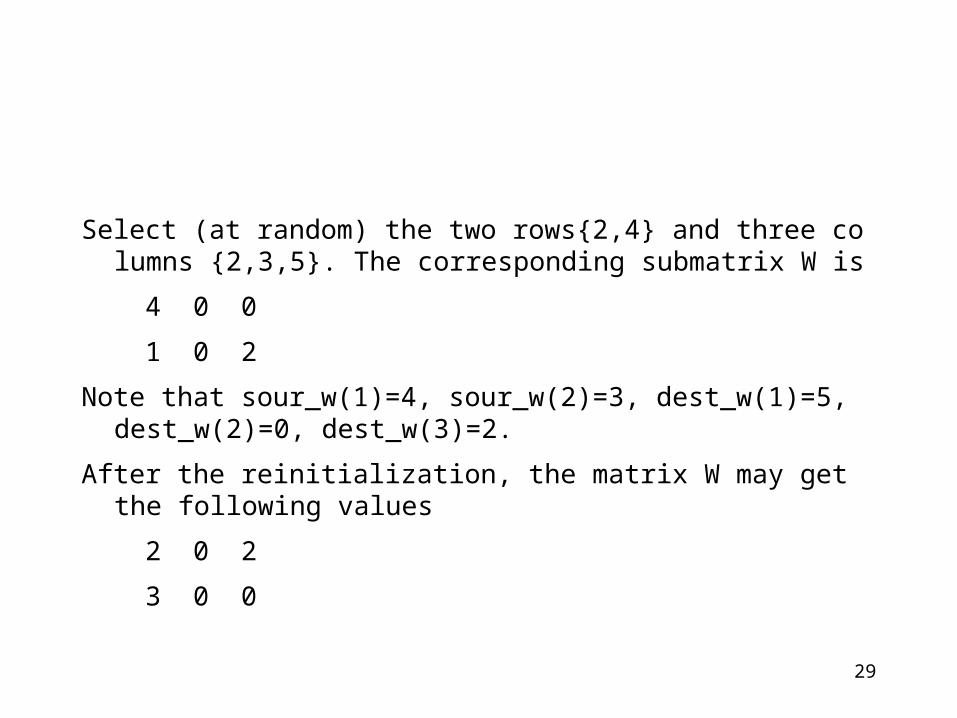
Select (at random) the two rows{2,4} and three columns {2,3,5}. The corresponding submatrix W is
4 0 0 1 0 2Note that sour_w(1)=4, sour_w(2)=3, dest_w(1)=5, dest_w
(2)=0, dest_w(3)=2.After the reinitialization, the matrix W may get the followin
g values 2 0 2 3 0 0
30
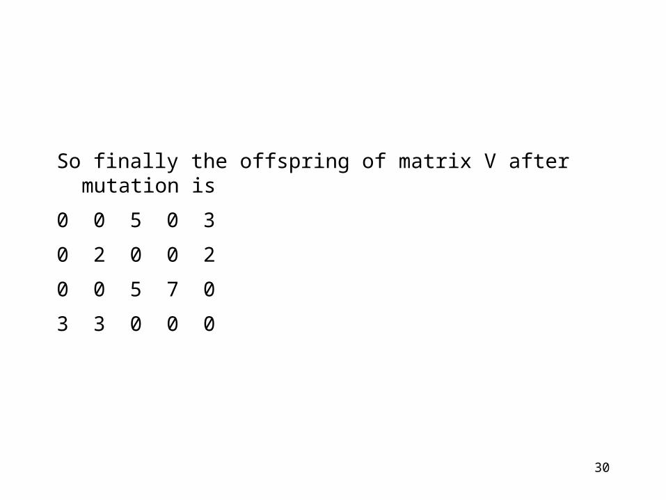
So finally the offspring of matrix V after mutation is
0 0 5 0 3
0 2 0 0 2
0 0 5 7 0
3 3 0 0 0
31
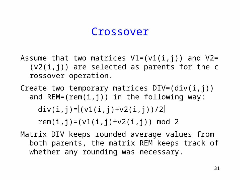
Crossover
Assume that two matrices V1=(v1(i,j)) and V2=(v2(i,j)) are selected as parents for the crossover operation.
Create two temporary matrices DIV=(div(i,j)) and REM=(rem(i,j)) in the following way:
div(i,j)=(v1(i,j)+v2(i,j))/2
rem(i,j)=(v1(i,j)+v2(i,j)) mod 2Matrix DIV keeps rounded average values from both paren
ts, the matrix REM keeps track of whether any rounding was necessary.
32
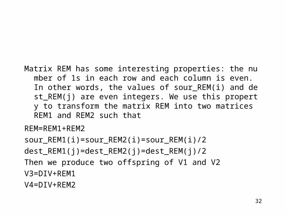
Matrix REM has some interesting properties: the number of 1s in each row and each column is even. In other words, the values of sour_REM(i) and dest_REM(j) are even integers. We use this property to transform the matrix REM into two matrices REM1 and REM2 such that
REM=REM1+REM2sour_REM1(i)=sour_REM2(i)=sour_REM(i)/2dest_REM1(j)=dest_REM2(j)=dest_REM(j)/2Then we produce two offspring of V1 and V2V3=DIV+REM1V4=DIV+REM2

33
Example
Given a problem with 4 sources and 5 destinations and the following constraints:
sour(1)=8, sour(2)=4, sour(3)=12, sour(4)=6dest(1)=3, dest(2)=5, dest(3)=10, dest(4)=7, dest(5)=5
34
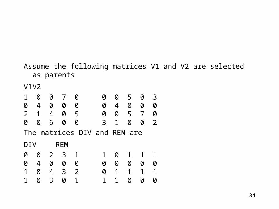
Assume the following matrices V1 and V2 are selected as parents
V1 V21 0 0 7 0 0 0 5 0 30 4 0 0 0 0 4 0 0 02 1 4 0 5 0 0 5 7 00 0 6 0 0 3 1 0 0 2The matrices DIV and REM are
DIV REM0 0 2 3 1 1 0 1 1 10 4 0 0 0 0 0 0 0 01 0 4 3 2 0 1 1 1 11 0 3 0 1 1 1 0 0 0
35
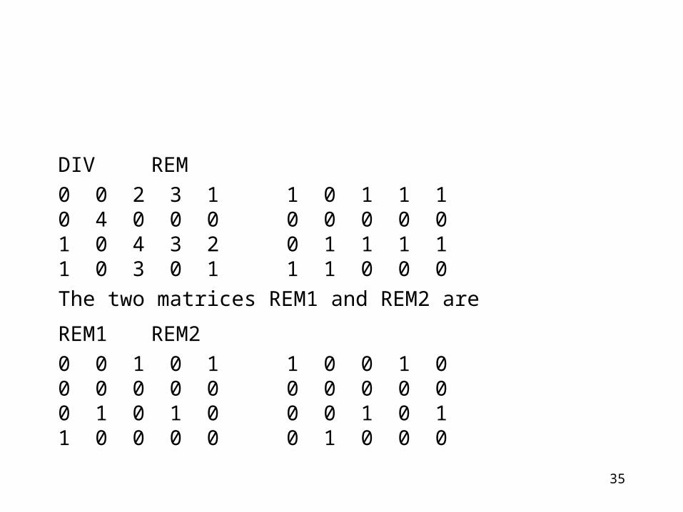
DIV REM0 0 2 3 1 1 0 1 1 10 4 0 0 0 0 0 0 0 01 0 4 3 2 0 1 1 1 11 0 3 0 1 1 1 0 0 0The two matrices REM1 and REM2 are
REM1 REM20 0 1 0 1 1 0 0 1 00 0 0 0 0 0 0 0 0 00 1 0 1 0 0 0 1 0 11 0 0 0 0 0 1 0 0 0
36
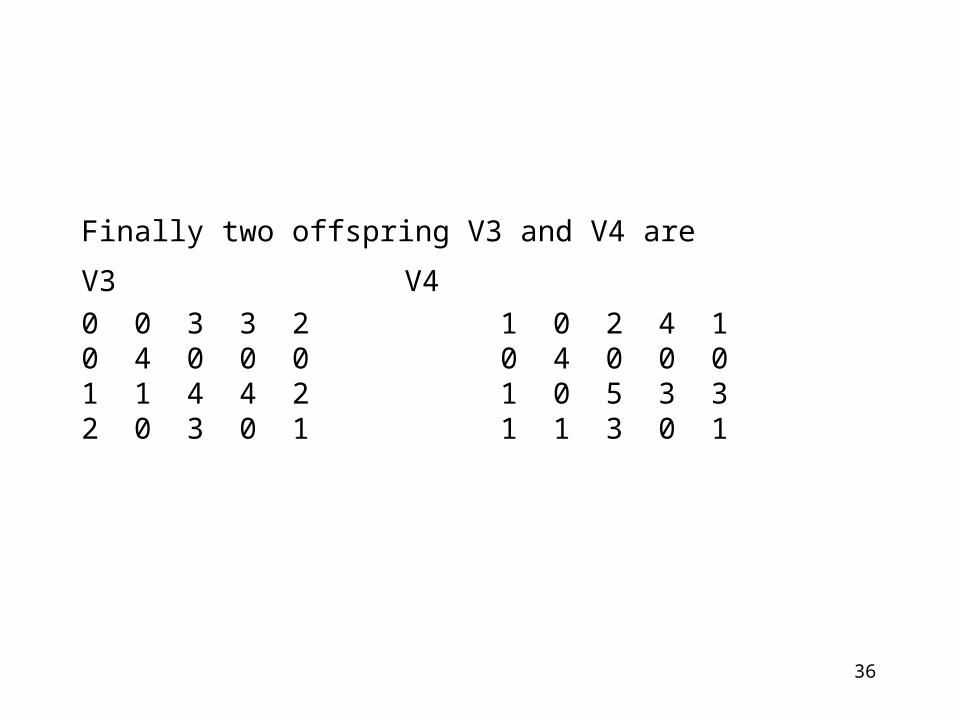
Finally two offspring V3 and V4 are
V3 V40 0 3 3 2 1 0 2 4 10 4 0 0 0 0 4 0 0 01 1 4 4 2 1 0 5 3 32 0 3 0 1 1 1 3 0 1
37
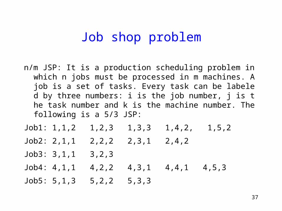
Job shop problem
n/m JSP: It is a production scheduling problem in which n jobs must be processed in m machines. A job is a set of tasks. Every task can be labeled by three numbers: i is the job number, j is the task number and k is the machine number. The following is a 5/3 JSP:
Job1: 1,1,2 1,2,3 1,3,3 1,4,2, 1,5,2Job2: 2,1,1 2,2,2 2,3,1 2,4,2Job3: 3,1,1 3,2,3Job4: 4,1,1 4,2,2 4,3,1 4,4,1 4,5,3Job5: 5,1,3 5,2,2 5,3,3
38
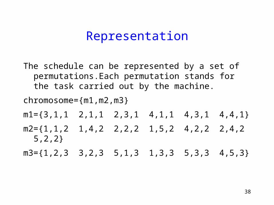
Representation
The schedule can be represented by a set of permutations.Each permutation stands for the task carried out by the machine.
chromosome={m1,m2,m3}
m1={3,1,1 2,1,1 2,3,1 4,1,1 4,3,1 4,4,1}
m2={1,1,2 1,4,2 2,2,2 1,5,2 4,2,2 2,4,2 5,2,2}
m3={1,2,3 3,2,3 5,1,3 1,3,3 5,3,3 4,5,3}
39
Fitness function
The total cost according to the chromosome
40
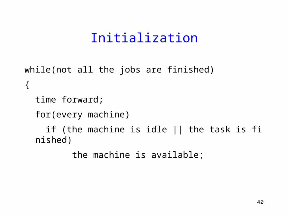
Initialization
while(not all the jobs are finished){ time forward; for(every machine) if (the machine is idle || the task is finished) the machine is available;
41
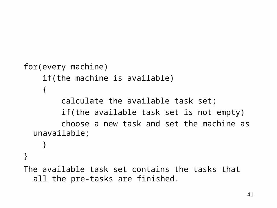
for(every machine) if(the machine is available) { calculate the available task set; if(the available task set is not empty) choose a new task and set the machine as
unavailable; }}
The available task set contains the tasks that all the pre-tasks are finished.
42
Genetic operators
Swap: any two elements of a machine can be swapped easily and check the feasibility
Modified-OX: choose the crossover points in one machine and calculate the similar crossover points (the beginning time is similar for the first point while the ending time is similar for the second point) for other machines. Then do like normal OX operator.