1 Traffic Analysis

8/11/2019 1 Traffic Analysis

http://slidepdf.com/reader/full/1-traffic-analysis 1/20

TRAFFIC ANALYSIS



Arrival Distributions

• The most fundamental assumption of classical traffic analysis is

that call arrivals are independent.

• An arrival from one source is unrelated to an arrival from any

other source.• Even though this assumption may be invalid in some instances,

it has general usefulness for most applications.

• In those cases where call arrivals tend to be correlated, useful

results can still be obtained by modifying a random arrival

analysis.• In this manner the random arrival assumption provides a

mathematical formulation that can be adjusted to produce

approximate solutions to problems that are otherwise

mathematically intractable.



Negative Exponential Inter-arrival Times

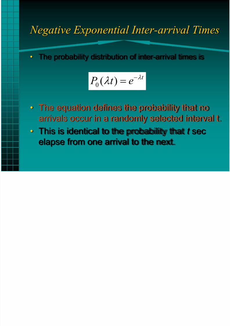
• The probability distribution of inter-arrival times is

• The equation defines the probability that no

arrivals occur in a randomly selected interval t. • This is identical to the probability that t sec

elapse from one arrival to the next.

0 ( ) t P t e



Example

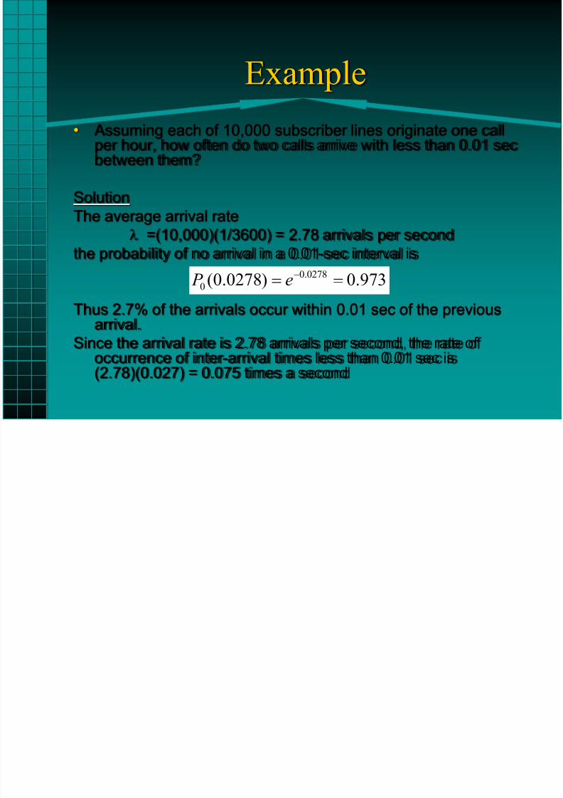
• Assuming each of 10,000 subscriber lines originate one callper hour, how often do two calls arrive with less than 0.01 secbetween them?

SolutionThe average arrival rate

=(10,000)(1/3600) = 2.78 arrivals per second

the probability of no arrival in a 0.01-sec interval is

Thus 2.7% of the arrivals occur within 0.01 sec of the previousarrival.

Since the arrival rate is 2.78 arrivals per second, the rate ofoccurrence of inter-arrival times less than 0.01 sec is(2.78)(0.027) = 0.075 times a second

0.0278

0 (0.0278) 0.973 P e



Negative Exponential Inter-arrival Times

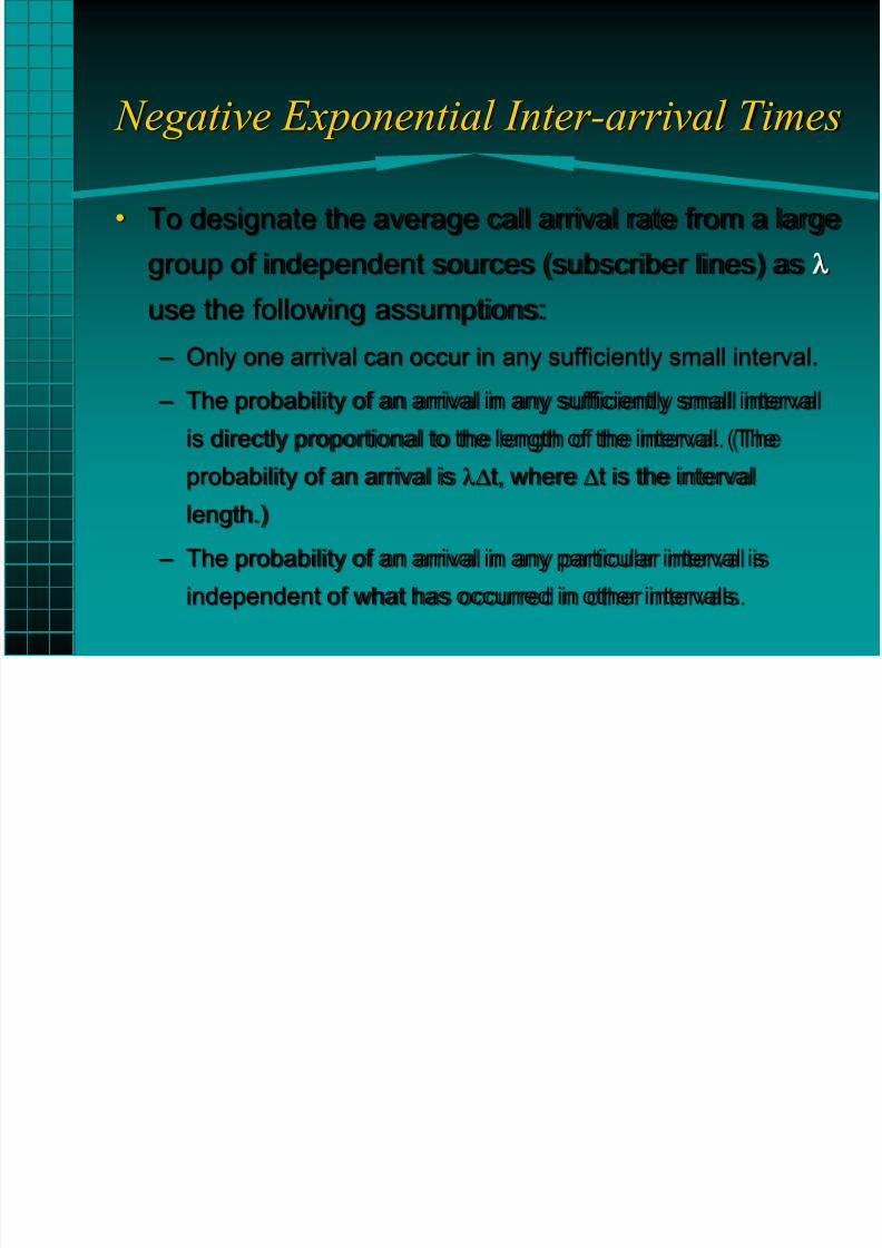
• To designate the average call arrival rate from a large

group of independent sources (subscriber lines) as

use the following assumptions:

– Only one arrival can occur in any sufficiently small interval.

– The probability of an arrival in any sufficiently small interval

is directly proportional to the length of the interval. (The

probability of an arrival is t, where t is the interval

length.)

– The probability of an arrival in any particular interval is

independent of what has occurred in other intervals.



Negative Exponential Interarrival Times

• The first two assumptions made in deriving the negative

exponential arrival distribution, can be intuitively justified for

most applications.

• The third assumption implies certain aspects of the sources that

cannot always be supported.

• First, certain events, such as television commercial breaks

might stimulate the sources to place their calls at nearly the

same time. In this case the negative exponential distribution

may still hold, but for a much higher calling rate during the

commercial.




• A more subtle implication of the independent arrival assumptioninvolves the number of sources, and not just their callingpatterns.

• When the probability of an arrival in any small time interval is

independent of other arrivals, it implies that the number ofsources available to generate requests is constant.

• If a number of arrivals occur immediately before any subintervalin question, some of the sources become busy and cannotgenerate requests.

• The effect of busy sources is to reduce the average arrival rate.

• Thus the inter-arrival times are always somewhat larger thanwhat the equation predicts them to be.

• The only time the arrival rate is truly independent of sourceactivity is when an infinite number of sources exist.




• If the number of sources is large and their average activity isrelatively low, busy sources do not appreciably reduce thearrival rate.

• For example, consider an end office that services 10.000

subscribers with 0.1 erlangs of activity each.• Normally, there are 1000 active links and 9000 subscribers

available to generate new arrivals.

• If the number of active subscribers increases by an unlikely50% to 1500 active lines, the number of idle subscribersreduces to 8500, a change of only 5.6%.

• Thus the arrival rate is relatively constant over a wide range ofsource activity.

• Whenever the arrival rate is fairly constant for the entire rangeof normal source activity, an infinite source assumption is

justified.



Poisson Arrival Distribution

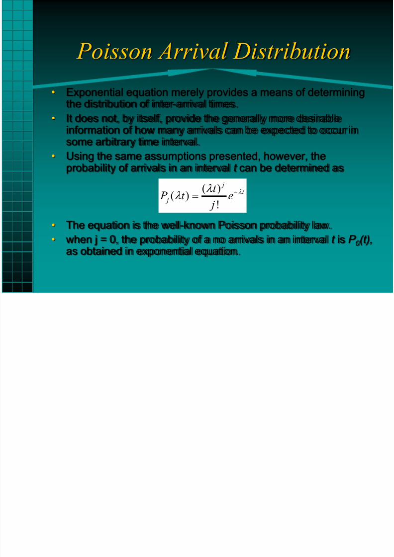
• Exponential equation merely provides a means of determiningthe distribution of inter-arrival times.

• It does not, by itself, provide the generally more desirableinformation of how many arrivals can be expected to occur insome arbitrary time interval.

• Using the same assumptions presented, however, theprobability of arrivals in an interval t can be determined as

• The equation is the well-known Poisson probability law.

• when j = 0, the probability of a no arrivals in an interval t is P 0 (t),as obtained in exponential equation.

( )( )

!

jt

j

t P t e

j



Poisson Arrival Distribution

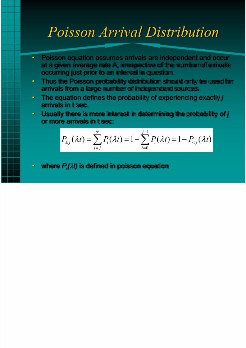
• Poisson equation assumes arrivals are independent and occurat a given average rate A, irrespective of the number of arrivalsoccurring just prior to an interval in question.

• Thus the Poisson probability distribution should only be used forarrivals from a large number of independent sources.

• The equation defines the probability of experiencing exactly jarrivals in t sec.

• Usually there is more interest in determining the probability of jor more arrivals in t sec:

• where P i ( t) is defined in poisson equation

1

0

( ) ( ) 1 ( ) 1 ( ) j

j i i j

i j i

P t P t P t P t



Example

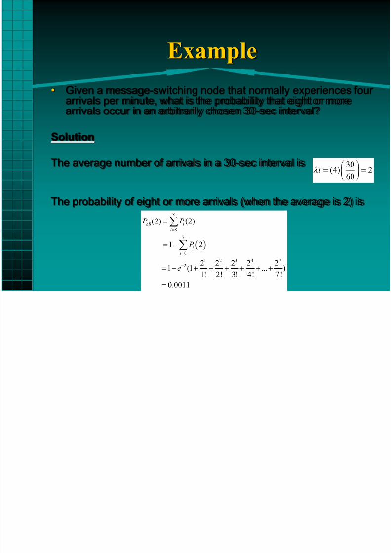
• Given a message-switching node that normally experiences fourarrivals per minute, what is the probability that eight or morearrivals occur in an arbitrarily chosen 30-sec interval?

Solution

The average number of arrivals in a 30-sec interval is

The probability of eight or more arrivals (when the average is 2) is

30(4) 2

60t

8

8

7

0

1 2 3 4 72

(2) (2)

1 2

2 2 2 2 21 (1 ... )

1! 2! 3! 4! 7!0.0011

i

i

i

i

P P

P

e



Example

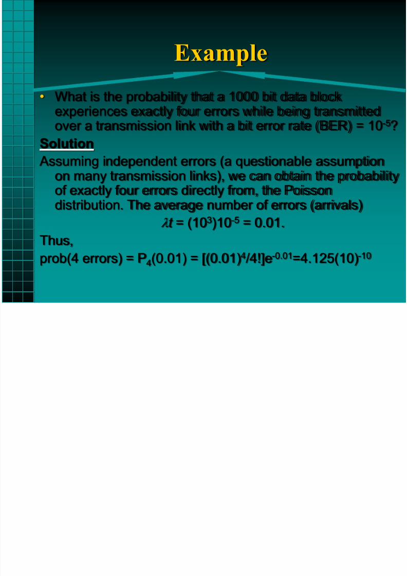
• What is the probability that a 1000 bit data blockexperiences exactly four errors while being transmittedover a transmission link with a bit error rate (BER) = 10-5?

Solution

Assuming independent errors (a questionable assumptionon many transmission links), we can obtain the probabilityof exactly four errors directly from, the Poissondistribution. The average number of errors (arrivals)

t = (103)10-5 = 0.01.

Thus,

prob(4 errors) = P4(0.01) = [(0.01)4/4!]e-0.01=4.125(10)-10



Holding Time Distributions

• The second factor of traffic intensity is the averageholding time t m.

• In some cases the average of the holding times is all

that needs to be known about holding times todetermine blocking probabilities in a loss system ordelays in a delay system.

• In other cases it is necessary to know the probabilitydistribution of the holding times to obtain the desiredresults.

• The two most commonly assumed holding timedistributions are: – constant holding times

– exponential holding times.



Constant Holding Times

• Constant holding times cannot be assumed forconventional voice conversations

• It is a reasonable assumption for such activities as

per-call call processing requirements, interofficeaddress signaling, operator assistance, and recordedmessage playback.

• Constant holding times are obviously valid fortransmission times in fixed length packet networks.

• When constant holding time messages are in effect,it is straightforward to use Poison equation todetermine the probability distribution of activechannels.



Constant Holding Times

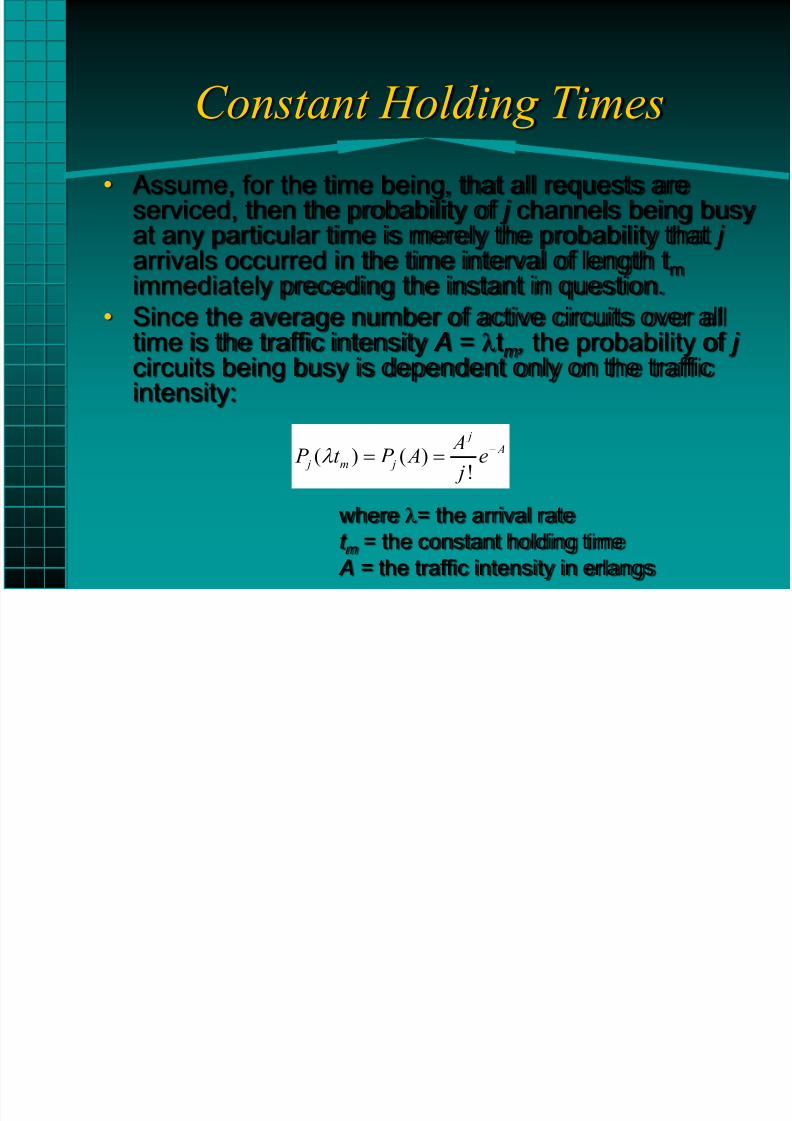
• Assume, for the time being, that all requests areserviced, then the probability of j channels being busyat any particular time is merely the probability that jarrivals occurred in the time interval of length t

m

immediately preceding the instant in question.

• Since the average number of active circuits over alltime is the traffic intensity A = tm, the probability of j circuits being busy is dependent only on the trafficintensity:

where = the arrival rate

t m = the constant holding time

A = the traffic intensity in erlangs

( ) ( )!

j A

j m j

A P t P A e

j



Exponential Holding Times

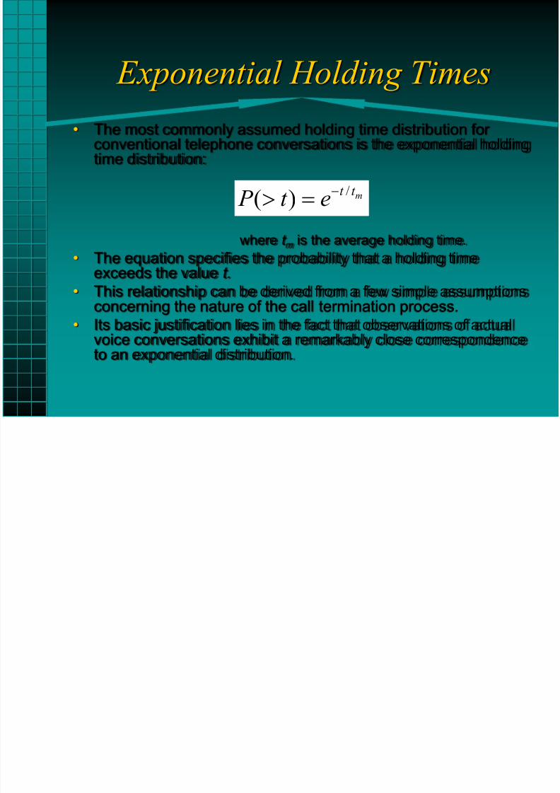
• The most commonly assumed holding time distribution forconventional telephone conversations is the exponential holdingtime distribution:

where t m is the average holding time.

• The equation specifies the probability that a holding timeexceeds the value t.

•This relationship can be derived from a few simple assumptionsconcerning the nature of the call termination process.

• Its basic justification lies in the fact that observations of actualvoice conversations exhibit a remarkably close correspondenceto an exponential distribution.

/( ) mt t P t e




• The exponential distribution possesses the curious property that

the probability of a termination is independent of how long a call

has been in progress.

• No matter how long a call has been in existence, the probability

of it lasting another t sec is defined by the equation

• In this sense exponential holding times represent the most

random process possible.• Not even knowledge of how long a call has been in progress

provides any information as to when the call will terminate.




• Combining a Poisson arrival process with an exponential holdingtime process to obtain the probability distribution of active circuitsis more complicated than it was for constant holding timesbecause calls can last indefinitely.

• The result proves to be dependent on only the average holdingtime.

• Thus the constant holding time equation is valid for exponentialholding times also (or any holding time distribution).

• The probability of j circuits being busy at any particular instant,

assuming a Poisson arrival process and that all requests areserviced immediately is

where A is the traffic intensity in erlangs.

This result is true for any distribution of holding times.

( )!

j A

j

A P A e

j



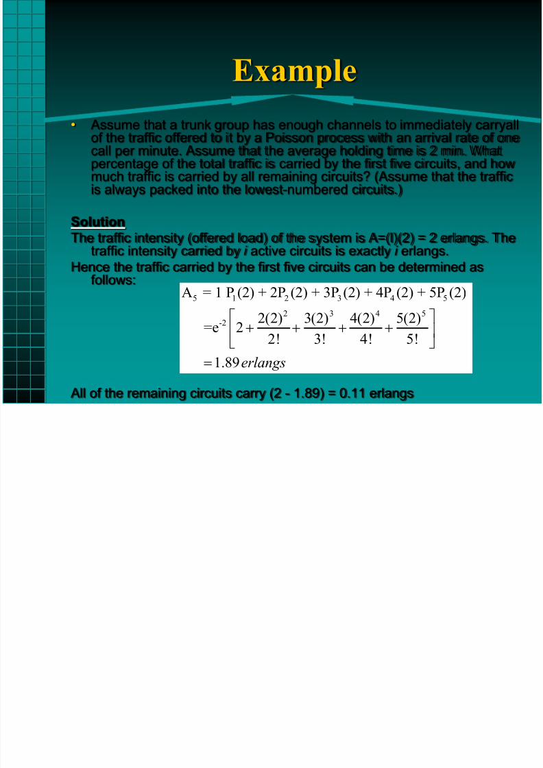
Example

• Assume that a trunk group has enough channels to immediately carryallof the traffic offered to it by a Poisson process with an arrival rate of onecall per minute. Assume that the average holding time is 2 min. Whatpercentage of the total traffic is carried by the first five circuits, and howmuch traffic is carried by all remaining circuits? (Assume that the traffic

is always packed into the lowest-numbered circuits.)

Solution

The traffic intensity (offered load) of the system is A=(l)(2) = 2 erlangs. Thetraffic intensity carried by i active circuits is exactly i erlangs.

Hence the traffic carried by the first five circuits can be determined as

follows:

All of the remaining circuits carry (2 - 1.89) = 0.11 erlangs

5 1 2 3 4 5

2 3 4 5-2

A = 1 P (2) + 2P (2) + 3P (2) + 4P (2) + 5P (2)

2(2) 3(2) 4(2) 5(2)=e 2

2! 3! 4! 5!

1.89erlangs



Example

• The result of the Example demonstrates theprinciple of diminishing returns as thecapacity of a system is increased to carrygreater and greater percentages of theoffered traffic.

• The first five circuits in the example carry94.5% of the traffic while all remainingcircuits carry only 5.5% of the traffic.

• If there are 100 sources. 95 extra circuits areneeded to carry the 5.5%.

Documents

1 Traffic Analysis