1

Toward Efficient Online Scheduling forDistributed Machine Learning Systems

Menglu Yu, Jia Liu Senior Memeber, IEEE , Chuan Wu Senior Memeber, IEEE , Bo Ji SeniorMemeber, IEEE Elizabeth S. Bentley Member, IEEE

Abstract—Recent years have witnessed a rapid growth of distributed machine learning (ML) frameworks, which exploit the massiveparallelism of computing clusters to expedite ML training. However, the proliferation of distributed ML frameworks also introduces manyunique technical challenges in computing system design and optimization. In a networked computing cluster that supports a largenumber of training jobs, a key question is how to design efficient scheduling algorithms to allocate workers and parameter serversacross different machines to minimize the overall training time. Toward this end, in this paper, we develop an online schedulingalgorithm that jointly optimizes resource allocation and locality decisions. Our main contributions are three-fold: i) We develop a newanalytical model that considers both resource allocation and locality; ii) Based on an equivalent reformulation and observations on theworker-parameter server locality configurations, we transform the problem into a mixed packing and covering integer program, whichenables approximation algorithm design; iii) We propose a meticulously designed approximation algorithm based on randomizedrounding and rigorously analyze its performance. Collectively, our results contribute to the state of the art of distributed ML systemoptimization and algorithm design.

Index Terms—Online resource scheduling, distributed machine learning, approximation algorithm

F

1 INTRODUCTION

Fueled by the rapid growth of data analytics and machinelearning (ML) applications, recent years have witnessedan ever-increasing hunger for computing power. However,with hardware capability no longer advancing at the pace ofthe Moore’s law, it has been widely recognized that a viablesolution to sustain such computing power needs is to exploitparallelism at both machine and chip scales. Indeed, therecent success of deep neural networks (DNN) is enabledby the use of distributed ML frameworks, which exploitthe massive parallelism over computing clusters with alarge number of GPUs. These distributed ML frameworkshave significantly accelerated the training of DNN for manyapplications (e.g., image and voice recognition, natural lan-guage processing, etc.). To date, prevailing distributed MLframeworks include TensorFlow [1], MXNet [2], PyTorch [3],Caffe [4], to name just a few.

However, the proliferation of distributed ML frame-works also introduces many unique technical challenges onlarge-scale computing system design and network resourceoptimization. Particularly, due to the decentralized nature,at the heart of distributed learning system optimization liesthe problem of scheduling ML jobs and resource provision-ing across different machines to minimize the total training

Menglu Yu is with the Department of Computer Science, Iowa State Univer-sity, Ames, IA 50011, USA (e-mail: mengluy@iastate.edu).Jia Liu is with the Department of Electrical and Computer Engineering, TheOhio State University, Columbus, OH 43210, USA (e-mail: liu@ece.osu.edu).Bo Ji is with the Department of Computer Science, Virginia Tech, Blacksburg,VA 24061, USA (e-mail: boji@vt.edu).Chuan Wu is with the Department of Computer Science, The University ofHong Kong, Hong Kong (e-mail: cwu@cs.hku.hk).Elizabeth S. Bentley is with the Air Force Research Laboratory, InformationDirectorate, Rome, NY 13441, USA (e-mail: elizabeth.bentley.3@us.af.mil).Digital Object Identifier xx.xxxx/XXXX.xxxx.xxxxx.

time. Such scheduling problems involve dynamic and com-binatorial worker and parameter server allocations, whichare inherently NP-hard. Also, the allocations of workers andparameter servers should take locality into careful consider-ation, since co-located workers and parameter servers canavoid costly network communication overhead. However,locality optimization adds yet another layer of difficulty inscheduling algorithm design. Exacerbating the problem isthe fact that the future arrival times of training jobs at an MLcomputing cluster are hard to predict, which necessitatesonline algorithm design without the knowledge of futurejob arrivals. So far in the literature, there remains a lackof holistic theoretical studies that address all the aforemen-tioned challenges. Most of the existing scheduling schemesare based on simple heuristics without performance guar-antee (see Section 2 for detailed discussions). This motivatesus to fill this gap and pursue efficient online schedulingdesigns for distributed ML resource optimization, whichoffer provable performance guarantee.

The main contribution of this paper is that we developan online scheduling algorithmic framework that jointlyyields resource scheduling and locality optimization deci-sions with strong competitive ratio performance. Further,we reveal interesting insights on how distributed ML frame-works affect online resource scheduling optimization. Ourmain technical results are summarized as follows:• By abstracting the architectures of prevailing dis-tributed ML frameworks, we formulate an online resourcescheduling optimization problem that: i) models the train-ing of ML jobs based on the parameter server (PS) ar-chitecture and stochastic gradient descent (SGD) method;and ii) explicitly takes locality optimization into consid-eration. We show that, due to the heterogeneous internal(between virtual machines or containers) and external (be-

arX

iv:2

108.

0291

7v2

[cs

.DC

] 1

4 A

ug 2

021

2

tween physical machines) communications, the locality-aware scheduling problem contains non-deterministic con-straints and is far more complex compared to the existingworks that are locality-oblivious (see, e.g., [5], [6]).• To solve the locality-aware scheduling problem, we de-velop an equivalent problem reformulation to enablesubsequent developments of online approximation algo-rithms. Specifically, upon carefully examining the localityconfigurations of worker-server relationships, we are ableto transform the original problem to a special-structuredinteger nonlinear program with mixed cover/packing-type constraints, and the low-complexity approximationalgorithm design with provable performance can be fur-ther entailed.• To tackle the integer nonlinear problem with mixedcover/packing-type constraints, we propose an approx-imation algorithm based on a meticulously designed ran-domized rounding scheme and then rigorously prove itsperformance. We note that the results of our randomizedrounding scheme are general and could be of independenttheoretical interest. Finally, by putting all algorithmic de-signs together, we construct a primal-dual online resourcescheduling (PD-ORS) scheme, which has an overall com-petitive ratio that only logarithmically depends on ML jobcharacteristics (e.g., required epochs, training samples).Collectively, our results contribute to a comprehensive

and fundamental understanding of distributed machinelearning system optimization. The remainder of this paperis organized as follows. In Section 2, we review the literatureto put our work in comparative perspectives. Section 3introduces the system model and problem formulation.Section 4 presents our algorithms and their performanceanalysis. Section 5 presents numerical results and Section 6concludes this paper.

2 RELATED WORK

As mentioned in Section 1, due to the high computa-tional workload of ML applications, many distributed MLframeworks (e.g., TensorFlow [1], MXNet [2], PyTorch [3],Caffe [4]) have been proposed to leverage modern large-scale computing clusters. A common distributed trainingarchitecture implemented in these distributed ML frame-works is the PS architecture [7], [8], which employs mul-tiple workers and PSs (implemented as virtual machinesor containers) to collectively train a global ML model.Coupled with the iterative ML training based on stochasticgradient descent (SGD), the interactions between machinesin the distributed ML cluster are significantly differentfrom those in traditional cloud computing platforms (e.g.,MapReduce [9] and Dryad [10] and references therein). Forexample, a MapReduce job usually partitions the input datainto independent chunks, which are then processed by themap step in a parallel fashion. The output of the maps arethen fed to the reduce step to be aggregated to yield thefinal result. Clearly, the data flows in MapReduce are a“one-way traffic”, which is unlike those iterative data flowsin ML training jobs whose completions highly depend onthe ML job’s convergence property. As a result, existing jobscheduling algorithms for cloud systems are not suitable fordistributed ML frameworks.

Among distributed ML system studies, most of the earlyattempts (see, e.g., [7], [8] and references therein) only con-sidered static allocation of workers and parameter servers.To our knowledge, the first work on understanding theperformance of distributed ML frameworks is [11], whereYan et al. developed analytical models to quantify the im-pacts of model-data partitioning and system provisioningfor DNN. Subsequently, Chun et al. [5] developed heuris-tic dynamic system reconfiguration algorithms to allocateworkers and parameter servers to minimize the runtime, butwithout providing optimality guarantee. The first dynamicdistributed scheduling algorithm with optimality guaranteewas reported in [12], where Sun et al. used standard mixedinteger linear program (MILP) solver to dynamically com-pute the worker-parameter server partition solutions. Dueto NP-hardness of the MILP, the scalability of this approachis limited. The most recent work [13] proposed an onlinescheduling algorithm to schedule synchronous training jobsin ML clusters with the goal to minimize the weightedcompletion time. However, the consecutive time slots wereallocated for each training job, and the numbers of workersand parameter servers could not be adjusted.

Another line of the research is to leverage the learning-based approach to do the resource scheduling. There are anumber of recent works using deep reinforcement learning(DRL) for resource allocation, device placement, and videostreaming. For example, Mao et al. [14] and Chen et al. [15]designed a multi-resource cluster scheduler using DRL withthe goal to minimize average job slowdown. The proposedscheduler picks one or more of the waiting jobs in the queueand allocate to machines at each time slot, and the resourcedemand of each job is unknown until after its arrival. Later,Mao et al. [16], [17] used DRL to heuristically train schedul-ing policies for graph-based parallel jobs by setting both par-allelism level and execution order. Meanwhile, Mirhoseiniet al. [18], [19] utilized DRL to design a model for efficientplacement of computational graphs onto hardware devices,aiming at minimize the running time of each individualTensorFlow job. Although various performance gains havebeen empirically reported, these DRL-based studies do notoffer optimality performance guarantee due to the lack oftheoretical foundation of DRL as of today.

The most relevant work to ours is [6], where Bao et al.developed an online primal-dual approximation algorithm,OASiS, to solve the scheduling problem for distributed MLsystems. Our work differs from [6] in the following keyaspects: 1) In [6], the workers and parameter servers areallocated on two strictly separated sets of physical machines,i.e., no worker and parameter server can share the samephysical machine, which significantly simplified the un-derlying optimization problem. In this work, we considerthe cases that workers and parameter servers can be co-located on the same physical machine, which is the commonpractice in existing ML systems (see, e.g., [20], [21]). Suchco-location can significantly reduce inter-server communica-tion, expedite training, and improve resource utilization effi-ciency between workers and parameter servers. However, aswill be shown later, the co-location setting leads to an inte-ger non-convex optimization problem with non-deterministicconstraints, which is much harder and necessitates newalgorithm design. 2) Ref. [6] advocates dynamic worker

3

......

...... PSM

Gradients Parameters

Parameter Server Worker

Database for Training Dataset

W1 W2 WN

PS1

Fig. 1: Illustration of distributedtraining with the PS architecture.

...

...

W1

WN

PSM

PS1

Time

Time

Time

Time

Gradients

Gradients

Gradients

Gradients

Param

eters

Param

eters

Param

eters

Param

eters

Time for training a mini-batch

Fig. 2: The workflow of iterativetraining.

Machine 4

Machine 1 Machine 2

Machine 5

Machine 3

Machine 6

Job 1 Job 2 Job 3

b(i)1

PS1

W1 W1 W2 W5 PS1

PS2

W2PS2

W1 W4PS1W3 W3

W3

W3

b(e)1

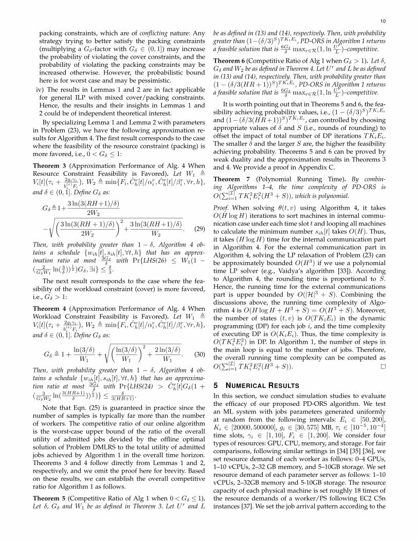
Fig. 3: Colocated parameter serversand workers on physical machines.

number adjustment, but does not guarantee the same globalbatch size across the training iterations. According to recentliterature [22], maintaining a consistent global batch size isimportant for ensuring convergence of DNN training, whenthe worker number varies. We ensure a consistent globalbatch size in our model. We note that the co-location settingwas considered in [23]. However, the scheduling algorithmtherein is a heuristic and does not provide performanceguarantee. This motivates us to develop new algorithmswith provable performance to fill this gap.

3 SYSTEM MODEL AND PROBLEM FORMULATION

In this section, we first provide a quick overview on thearchitecture of distributed ML frameworks to familiarizereaders with the necessary background. Then, we will in-troduce our analytical models for ML jobs and resourceconstraints, as well as the overall problem formulation.

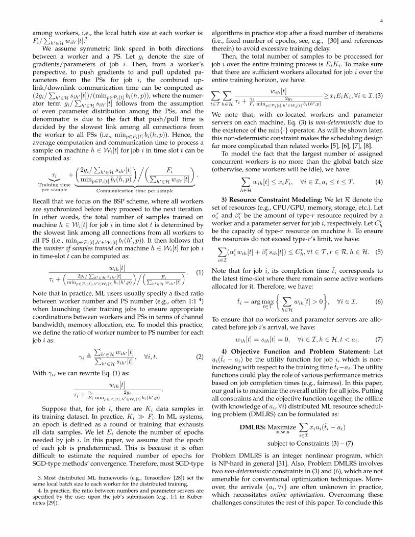
1) Distributed Machine Learning: A Primer. As illus-trated in Fig. 1, the key components of a PS-based dis-tributed ML system include parameter servers, workers,and the training dataset, which are usually implementedover a connected computing cluster that contains multiplephysical machines. The training dataset of an ML job isstored in distributed data storage (e.g., HDFS [24]) andusually divided into equal-sized data chunks. Each datachunk further contains multiple equal-sized mini-batches.

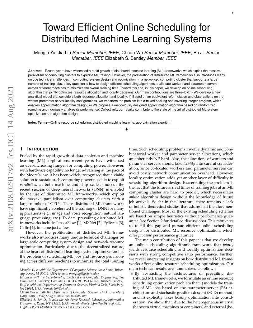
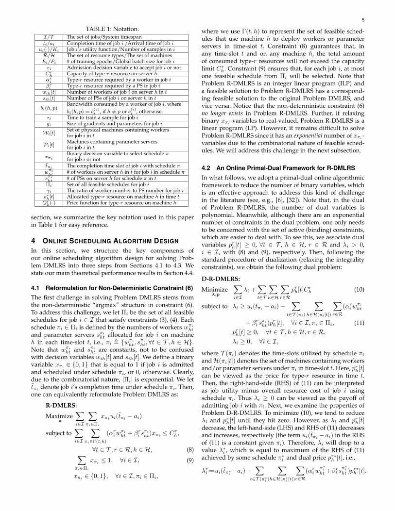
To date, one of the most widely adopted training algo-rithms in distributed ML frameworks is the stochastic gra-dient descent method (SGD) [25]. With SGD, the interactionsbetween workers and parameter servers are illustrated inFig 2. A worker is loaded with the DNN model (we focuson data parallel training) with current values of the modelparameters (e.g., the weights of a DNN) and retrieves anew data chunk from the data storage. In each trainingiteration, a worker processes one mini-batch from its datachunk to compute gradients (i.e., directions and magnitudesof parameter changes).1 Upon finishing a mini-batch, theworker sends the gradients to the parameter servers, re-ceives updated global parameters, and then continues withthe next training iteration to work on the next mini-batch.On the parameter server side, parameters are updated as:w[k] = w[k − 1] + αkg[k], where w[k], αk, and g[k] denotethe parameter values, step-size, and stochastic gradient inthe k-th update, respectively.

1. As an example, in a DNN model, gradients can be computed bythe well-known “back-propagation” approach.

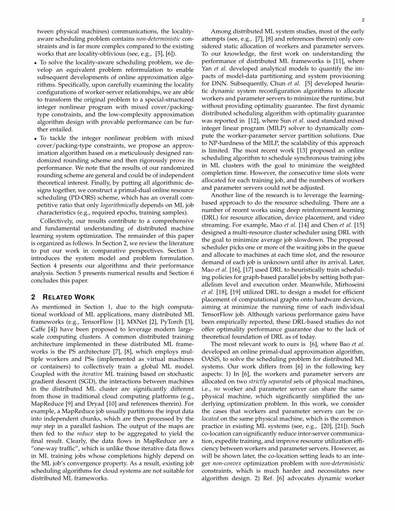
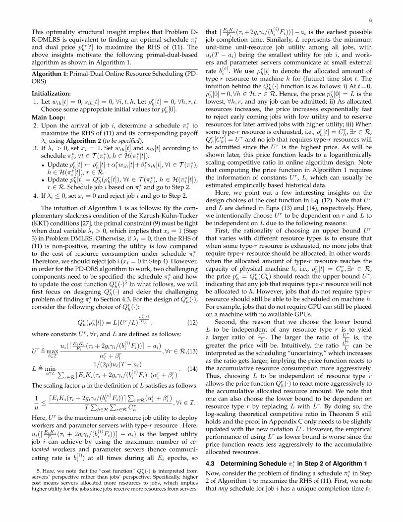
2) Modeling of Learning Jobs: We consider a time-slotted system. The scheduling time-horizon is denoted as Twith |T | = T . We use I to represent the set of training jobsand let ai denote the arrival time-slot of job i ∈ I . As shownin Fig. 3, parameter servers and workers could spread overmultiple physical machines. We let H represent the set ofphysical machines. For each job i, we use wih[t], sih[t] ≥ 0 torepresent the allocated numbers of workers and parameterservers on machine h ∈ H in each time-slot t ≥ ai,respectively. Further, we let Pi[t] , {h ∈ H|sih[t] > 0} andWi[t] , {h ∈ H|wih[t] > 0} denote the sets of physicalmachines that contain parameter servers and workers forjob i in time-slot t, respectively.

We use a binary variable xi ∈ {0, 1} to indicate whetherjob i is admitted (xi = 1) or not (xi = 0). We use τi todenote the training for each sample of job i. We let bi(h, p)denote the data rate of the link between a worker for jobi (on machine h) and a parameter server (on machine p).Each worker or parameter server is exclusively assignedto some job i, and bi(h, p) is reserved and decided by theuser upon job submission, which is common to ensure thedata transfer performance [6]. Note that the value of bi(h, p)is locality-dependent where the slowest worker will becomethe bottleneck since we focus on Bulk-Synchronous-Parallel(BSP) scheme [26]. Specifically, we have:

bi(h, p) =

{b(i)i , if h = p,

b(e)i , otherwise,

where b(i)i and b(e)i denote the internal and external com-

munication link rates, respectively. For example, as shownin Fig. 3, since Job 1’s worker W4 and parameter serverPS2 are both on the same machine, they communicate atthe internal link rate b

(i)1 . On the other hand, since Job

1’s worker W3 and parameter server PS2 are on differentphysical machines, they communicate at the external linkrate b(e)1 . In practice, it usually holds that b(e)i � b

(i)i .

Next, we calculate the amount of time for a workeron machine h to process a sample. We use Fi to denotethe global batch size of job i, which is a fixed constantacross all time-slots.2 We assume Fi is equally divided

2. We note that this fixed global batch size requirement is compli-ant with the standard SGD implementation [27] and important forensuring convergence [22]. In contrast, the global batch size in someexisting works on dynamic ML resource allocation (e.g., [6]) could betime-varying, which necessitates time-varying dynamic learning rateadjustments to offset correspondingly and further complicates the SGDimplementation.

4

among workers, i.e., the local batch size at each worker is:Fi/

∑h′∈H wih′ [t].

3

We assume symmetric link speed in both directionsbetween a worker and a PS. Let gi denote the size ofgradients/parameters of job i. Then, from a worker’sperspective, to push gradients to and pull updated pa-rameters from the PSs for job i, the combined up-link/downlink communication time can be computed as:(2gi/

∑h′∈H sih′ [t])/(minp∈Pi[t] bi(h, p)), where the numer-

ator term gi/∑h′∈H sih′ [t] follows from the assumption

of even parameter distribution among the PSs, and thedenominator is due to the fact that push/pull time isdecided by the slowest link among all connections fromthe worker to all PSs (i.e., minp∈Pi[t] bi(h, p)). Hence, theaverage computation and communication time to process asample on machine h ∈ Wi[t] for job i in time slot t can becomputed as:

τi︸︷︷︸Training time

per sample

+

(2gi/

∑h′∈H sih′ [t]

minp∈Pi[t] bi(h, p)

)/(Fi∑

h′∈H wih′ [t]

)︸ ︷︷ ︸

Communication time per sample

.

Recall that we focus on the BSP scheme, where all workersare synchronized before they proceed to the next iteration.In other words, the total number of samples trained onmachine h ∈ Wi[t] for job i in time slot t is determined bythe slowest link among all connections from all workers toall PS (i.e., minp∈Pi[t],h′∈Wi[t] bi(h

′, p)). It then follows thatthe number of samples trained on machine h ∈ Wi[t] for job iin time-slot t can be computed as:

wih[t]

τi +(

2gi/∑h′∈H sih′ [t]

minp∈Pi[t],h′∈Wi[t] bi(h′,p)

)/(Fi∑

h′∈H wih′ [t]

) . (1)

Note that in practice, ML users usually specify a fixed ratiobetween worker number and PS number (e.g., often 1:1 4)when launching their training jobs to ensure appropriatecoordinations between workers and PSs in terms of channelbandwidth, memory allocation, etc. To model this practice,we define the ratio of worker number to PS number for eachjob i as:

γi ,

∑h′∈H wih′ [t]∑h′∈H sih′ [t]

, ∀i, t. (2)

With γi, we can rewrite Eq. (1) as:

wih[t]

τi + γiFi

2giminp∈Pi[t],h′∈Wi[t] bi(h

′,p)

.

Suppose that, for job i, there are Ki data samples inits training dataset. In practice, Ki � Fi. In ML systems,an epoch is defined as a round of training that exhaustsall data samples. We let Ei denote the number of epochsneeded by job i. In this paper, we assume that the epochof each job is predetermined. This is because it is oftendifficult to estimate the required number of epochs forSGD-type methods’ convergence. Therefore, most SGD-type

3. Most distributed ML frameworks (e.g., Tensorflow [28]) set thesame local batch size to each worker for the distributed training.

4. In practice, the ratio between numbers and parameter servers arespecified by the user upon the job’s submission (e.g., 1:1 in Kuber-netes [29]).

algorithms in practice stop after a fixed number of iterations(i.e., fixed number of epochs, see, e.g., [30] and referencestherein) to avoid excessive training delay.

Then, the total number of samples to be processed forjob i over the entire training process is EiKi. To make surethat there are sufficient workers allocated for job i over theentire training horizon, we have:∑t∈T

∑h∈H

wih[t]

τi + γiFi

2giminp∈Pi[t],h′∈Wi[t] bi(h

′,p)

≥xiEiKi,∀i ∈ I. (3)

We note that, with co-located workers and parameterservers on each machine, Eq. (3) is non-deterministic due tothe existence of the min{·} operator. As will be shown later,this non-determistic constraint makes the scheduling designfar more complicated than related works [5], [6], [7], [8].

To model the fact that the largest number of assignedconcurrent workers is no more than the global batch size(otherwise, some workers will be idle), we have:∑

h∈Hwih[t] ≤ xiFi, ∀i ∈ I, ai ≤ t ≤ T. (4)

3) Resource Constraint Modeling: We let R denote theset of resources (e.g., CPU/GPU, memory, storage, etc.). Letαri and βri be the amount of type-r resource required by aworker and a parameter server for job i, respectively. Let Crhbe the capacity of type-r resource on machine h. To ensurethe resources do not exceed type-r’s limit, we have:∑i∈I

(αriwih[t] + βri sih[t]) ≤ Crh,∀t ∈ T , r ∈ R, h ∈ H. (5)

Note that for job i, its completion time ti corresponds tothe latest time-slot where there remain some active workersallocated for it. Therefore, we have:

ti = arg maxt∈T

{ ∑h∈H

wih[t] > 0

}, ∀i ∈ I. (6)

To ensure that no workers and parameter servers are allo-cated before job i’s arrival, we have:

wih[t] = sih[t] = 0, ∀i ∈ I, h ∈ H, t < ai. (7)

4) Objective Function and Problem Statement: Letui(ti − ai) be the utility function for job i, which is non-increasing with respect to the training time ti−ai. The utilityfunctions could play the role of various performance metricsbased on job completion times (e.g., fairness). In this paper,our goal is to maximize the overall utility for all jobs. Puttingall constraints and the objective function together, the offline(with knowledge of ai, ∀i) distributed ML resource schedul-ing problem (DMLRS) can be formulated as:

DMLRS: Maximizex,w,s

∑i∈I

xiui(ti − ai)

subject to Constraints (3) – (7).

Problem DMLRS is an integer nonlinear program, whichis NP-hard in general [31]. Also, Problem DMLRS involvestwo non-deterministic constraints in (3) and (6), which are notamenable for conventional optimization techniques. More-over, the arrivals {ai,∀i} are often unknown in practice,which necessitates online optimization. Overcoming thesechallenges constitutes the rest of this paper. To conclude this

5

TABLE 1: Notation.I/T The set of jobs/System timespanti/ai Completion time of job i /Arrival time of job i

ui(·)/Ki Job i’s utility function/Number of samples in iR/H The set of resource types/The set of machinesEi/Fi # of training epochs/Global batch size for job ixi Admission decision variable to accept job i or notCrh Capacity of type-r resource on server hαri Type-r resource required by a worker in job iβri Type-r resource required by a PS in job i

wih[t] Number of workers of job i on server h in tsih[t] Number of PSs of job i on server h in t

bi(h, p)Bandwidth consumed by a worker of job i, wherebi(h, p) = b

(e)i , if h 6= p or b(i)i , otherwise.

τi Time to train a sample for job igi Size of gradients and parameters for job i

Wi[t]Set of physical machines containing workersfor job i in t

Pi[t]Machines containing parameter serversfor job i in t

xπiBinary decision variable to select schedule πfor job i or not

tπi The completion time slot of job i with schedule πwπiht # of workers on server h in t for job i in schedule πsπiht # of PSs on server h for schedule π in t

Πi Set of all feasible schedules for job iγi The ratio of worker number to PS number for job iρrh[t] Allocated type-r resource on machine h in time tQrh(·) Price function for type-r resource on machine h

section, we summarize the key notation used in this paperin Table 1 for easy reference.

4 ONLINE SCHEDULING ALGORITHM DESIGN

In this section, we structure the key components ofour online scheduling algorithm design for solving Prob-lem DMLRS into three steps from Sections 4.1 to 4.3. Westate our main theoretical performance results in Section 4.4.

4.1 Reformulation for Non-Deterministic Constraint (6)The first challenge in solving Problem DMLRS stems fromthe non-deterministic “argmax” structure in constraint (6).To address this challenge, we let Πi be the set of all feasibleschedules for job i ∈ I that satisfy constraints (3), (4). Eachschedule πi ∈ Πi is defined by the numbers of workers wπihtand parameter servers sπiht allocated for job i on machineh in each time-slot t, i.e., πi , {wπiht , s

πiht,∀t ∈ T , h ∈ H}.

Note that wπiht and sπiht are constants, not to be confusedwith decision variables wih[t] and sih[t]. We define a binaryvariable xπi ∈ {0, 1} that is equal to 1 if job i is admittedand scheduled under schedule πi, or 0, otherwise. Clearly,due to the combinatorial nature, |Πi| is exponential. We lettπi denote job i’s completion time under schedule πi. Then,one can equivalently reformulate Problem DMLRS as:

R-DMLRS:

Maximizex

∑i∈I

∑πi∈Πi

xπiui(tπi − ai)

subject to∑i∈I

∑πi∈Γ(t,h)

(αriwπiht + βri s

πiht)xπi ≤ C

rh,

∀t ∈ T , r ∈ R, h ∈ H, (8)∑πi∈Πi

xπi ≤ 1, ∀i ∈ I, (9)

xπi ∈ {0, 1}, ∀i ∈ I, πi ∈ Πi,

where we use Γ(t, h) to represent the set of feasible sched-ules that use machine h to deploy workers or parameterservers in time-slot t. Constraint (8) guarantees that, inany time-slot t and on any machine h, the total amountof consumed type-r resources will not exceed the capacitylimit Crh. Constraint (9) ensures that, for each job i, at mostone feasible schedule from Πi will be selected. Note thatProblem R-DMLRS is an integer linear program (ILP) anda feasible solution to Problem R-DMLRS has a correspond-ing feasible solution to the original Problem DMLRS, andvice versa. Notice that the non-deterministic constraint (6)no longer exists in Problem R-DMLRS. Further, if relaxingbinary xπi -variables to real-valued, Problem R-DMLRS is alinear program (LP). However, it remains difficult to solveProblem R-DMLRS since it has an exponential number of xπi -variables due to the combinatorial nature of feasible sched-ules. We will address this challenge in the next subsection.

4.2 An Online Primal-Dual Framework for R-DMLRSIn what follows, we adopt a primal-dual online algorithmicframework to reduce the number of binary variables, whichis an effective approach to address this kind of challengein the literature (see, e.g., [6], [32]). Note that, in the dualof Problem R-DMLRS, the number of dual variables ispolynomial. Meanwhile, although there are an exponentialnumber of constraints in the dual problem, one only needsto be concerned with the set of active (binding) constraints,which are easier to deal with. To see this, we associate dualvariables prh[t] ≥ 0, ∀t ∈ T , h ∈ H, r ∈ R and λi > 0,i ∈ I , with (8) and (9), respectively. Then, following thestandard procedure of dualization (relaxing the integralityconstraints), we obtain the following dual problem:

D-R-DMLRS:

Minimizeλ,p

∑i∈I

λi +∑t∈T

∑h∈H

∑r∈R

prh[t]Crh (10)

subject to λi ≥ ui(tπi − ai)−∑

t∈T (πi)

∑h∈H(πi[t])

∑r∈R

(αriwπiht

+ βri sπiht)p

rh[t], ∀i ∈ I, πi ∈ Πi, (11)

prh[t] ≥ 0, ∀t ∈ T , h ∈ H, r ∈ R,λi ≥ 0, ∀i ∈ I,

where T (πi) denotes the time-slots utilized by schedule πiandH(πi[t]) denotes the set of machines containing workersand/or parameter servers under πi in time-slot t. Here, prh[t]can be viewed as the price for type-r resource in time t.Then, the right-hand-side (RHS) of (11) can be interpretedas job utility minus overall resource cost of job i usingschedule πi. Thus λi ≥ 0 can be viewed as the payoff ofadmitting job i with πi. Next, we examine the properties ofProblem D-R-DMLRS. To minimize (10), we tend to reduceλi and prh[t] until they hit zero. However, as λi and prh[t]decrease, the left-hand-side (LHS) and RHS of (11) decreasesand increases, respectively (the term ui(tπi − ai) in the RHSof (11) is a constant given πi). Therefore, λi will drop to avalue λ∗i , which is equal to maximum of the RHS of (11)achieved by some schedule π∗i and dual price pr∗h [t], i.e.,

λ∗i =ui(tπ∗i −ai)−∑

t∈T (π∗i )

∑h∈H(π∗i [t])

∑r∈R

(αriwπ∗iht +βri s

π∗iht )pr∗h [t].

6

This optimality structural insight implies that Problem D-R-DMLRS is equivalent to finding an optimal schedule π∗iand dual price pr∗h [t] to maximize the RHS of (11). Theabove insights motivate the following primal-dual-basedalgorithm as shown in Algorithm 1.

Algorithm 1: Primal-Dual Online Resource Scheduling (PD-ORS).

Initialization:1. Let wih[t] = 0, sih[t] = 0, ∀i, t, h. Let ρrh[t] = 0, ∀h, r, t.

Choose some appropriate initial values for prh[0].Main Loop:2. Upon the arrival of job i, determine a schedule π∗i to

maximize the RHS of (11) and its corresponding payoffλi using Algorithm 2 (to be specified).

3. If λi > 0, set xi = 1. Set wih[t] and sih[t] according toschedule π∗i , ∀t ∈ T (π∗i ), h ∈ H(π∗i [t]).• Update ρrh[t]← ρrh[t]+αriwih[t]+βri sih[t], ∀t ∈ T (π∗i ),h ∈ H(π∗i [t]), r ∈ R.

• Update prh[t] = Qrh(ρrh[t]), ∀t ∈ T (π∗i ), h ∈ H(π∗i [t]),r ∈ R. Schedule job i based on π∗i and go to Step 2.

4. If λi ≤ 0, set xi = 0 and reject job i and go to Step 2.

The intuition of Algorithm 1 is as follows: By the com-plementary slackness condition of the Karush-Kuhn-Tucker(KKT) conditions [27], the primal constraint (9) must be tightwhen dual variable λi > 0, which implies that xi = 1 (Step3) in Problem DMLRS. Otherwise, if λi = 0, then the RHS of(11) is non-positive, meaning the utility is low comparedto the cost of resource consumption under schedule π∗i .Therefore, we should reject job i (xi = 0 in Step 4). However,in order for the PD-ORS algorithm to work, two challengingcomponents need to be specified: the schedule π∗i and howto update the cost function Qrh(·)5 In what follows, we willfirst focus on designing Qrh(·) and defer the challengingproblem of finding π∗i to Section 4.3. For the design of Qrh(·),consider the following choice of Qrh(·):

Qrh(ρrh[t]) = L(Ur/L)ρrh[t]

Crh , (12)

where constants Ur , ∀r, and L are defined as follows:

Ur,maxi∈I

ui(dEiKiFi(τi + 2giγi/(b

(i)i Fi))e − ai)

αri + βri,∀r ∈ R,(13)

L , mini∈I

1/(2µ)ui(T − ai)∑r∈RdEiKi(τi + 2giγi/(b

(e)i Fi)e(αri + βri )

. (14)

The scaling factor µ in the definition of L satisfies as follows:

1

µ≤dEiKi(τi + 2giγi/(b

(e)i Fi))e

∑r∈R(αri + βri )

T∑h∈H

∑r∈R C

rh

,∀i ∈ I.

Here, Ur is the maximum unit-resource job utility to deployworkers and parameter servers with type-r resource . Here,ui(dEiKiFi

(τi + 2giγi/(b(i)i Fi))e − ai) is the largest utility

job i can achieve by using the maximum number of co-located workers and parameter servers (hence communi-cating rate is b

(i)i ) at all times during all Ei epochs, so

5. Here, we note that the “cost function” Qrh(·) is interpreted fromservers’ perspective rather than jobs’ perspective. Specifically, highercost means servers allocated more resources to jobs, which implieshigher utility for the jobs since jobs receive more resources from servers.

that dEiKiFi(τi+2giγi/(b

(i)i Fi))e−ai is the earliest possible

job completion time. Similarly, L represents the minimumunit-time unit-resource job utility among all jobs, withui(T − ai) being the smallest utility for job i, and work-ers and parameter servers communicate at small externalrate b

(e)i . We use ρrh[t] to denote the allocated amount of

type-r resource to machine h for (future) time slot t. Theintuition behind the Qrh(·) function is as follows: i) At t=0,ρrh[0] = 0,∀h ∈ H, r ∈ R. Hence, the price prh[0] = L is thelowest, ∀h, r, and any job can be admitted; ii) As allocatedresources increases, the price increases exponentially fastto reject early coming jobs with low utility and to reserveresources for later arrived jobs with higher utility; iii) Whensome type-r resource is exhausted, i.e., ρrh[t] = Crh,∃r ∈ R,Qrh[Crh] = Ur and no job that requires type-r resources willbe admitted since the Ur is the highest price. As will beshown later, this price function leads to a logarithmicallyscaling competitive ratio in online algorithm design. Notethat computing the price function in Algorithm 1 requiresthe information of constants Ur , L, which can usually beestimated empirically based historical data.

Here, we point out a few interesting insights on thedesign choices of the cost function in Eq. (12). Note that Ur

and L are defined in Eqns (13) and (14), respectively. Here,we intentionally choose Ur to be dependent on r and L tobe independent on L due to the following reasons:

First, the rationality of choosing an upper bound Ur

that varies with different resource types is to ensure thatwhen some type-r resource is exhausted, no more jobs thatrequire type-r resource should be allocated. In other words,when the allocated amount of type-r resource reaches thecapacity of physical machine h, i.e., ρrh[t] = Crn,∃r ∈ R,the price prh = Qrh(Crh) should reach the upper bound Ur ,indicating that any job that requires type-r resource will notbe allocated to h. However, jobs that do not require type-rresource should still be able to be scheduled on machine h.For example, jobs that do not require GPU can still be placedon a machine with no available GPUs.

Second, the reason that we choose the lower boundL to be independent of any resource type r is to yielda larger ratio of Ur

L . The larger the ratio of Ur

L is, thegreater the price will be. Intuitively, the ratio Ur

L can beinterpreted as the scheduling “uncertainty,” which increasesas the ratio gets larger, implying the price function reacts tothe accumulative resource consumption more aggressively.Thus, choosing L to be independent of resource type rallows the price function Qrh(·) to react more aggressively tothe accumulative allocated resource amount. We note thatone can also choose the lower bound to be dependent onresource type r by replacing L with Lr. By doing so, thelog-scaling theoretical competitive ratio in Theorem 5 stillholds and the proof in Appendix C only needs to be slightlyupdated with the new notation Lr . However, the empiricalperformance of using Lr as lower bound is worse since theprice function reacts less aggressively to the accumulativeallocated resources.

4.3 Determining Schedule π∗i in Step 2 of Algorithm 1Now, consider the problem of finding a schedule π∗i in Step2 of Algorithm 1 to maximize the RHS of (11). First, we notethat any schedule for job i has a unique completion time ti,

7

ps

w w

ps

w

(a) |Pi[t]| 6= 1.

ps

w w w

(b) |Pi[t]| = 1, |Wi[t]| 6= 1.

ps

w w

(c) |Pi[t]|=|Wi[t]|=1,Pi[t]6=Wi[t].

ps ps

w w

(d) |Pi[t]|=|Wi[t]|=1,Pi[t]=Wi[t].

Fig. 4: Values of 2giminp∈Pi[t],h∈Wi[t] bi(h,p)

under various settings of Pi[t] andWi[t]. Here, 2giminp∈Pi[t],h∈Wi[t] bi(h,p)

= 2 gi

b(i)i

if and

only if in (d).

including the maximizer π∗i for (11). Hence, the problem offinding the maximum RHS of (11) can be decomposed as:

Maxti

Maxw,s

ui(ti−ai)−∑t∈T

∑h∈H

∑r∈R

prh[t]

×(αriwih[t] + βri sih[t])

s.t. αriwih[t] + βri sih[t] ≤ Crh[t],∀t ∈ T , r ∈ R, h ∈ H,

Constraints (3)(4)(7) for xi = 1,

, (15)

where Crh[t] , Crh − ρrh[t]. Note that in the inner problem,ui(ti−ai) is a constant for any given ti. Thus, the innerproblem can be simplified as:

Minimizew,s

∑t∈[ai,ti]

∑h∈H

∑r∈R

prh[t](αriwih[t] + βri sih[t]) (16)

subject to∑

t∈[ai,ti]

∑h∈H

wih[t]

τi + γiFi

2giminp∈Pi[t],h′∈Wi[t] bi(h

′,p)

≥ Vi,

(17)

αriwih[t]+βri sih[t]≤ Crh[t],∀r, h,∀t∈ [ai, ti], (18)

Constraint (4) for all t ∈ [ai, ti],

where Vi , EiKi represents the total training workload (to-tal count of samples trained, where a sample is counted Eitimes if trained for Ei times). Note that in Problem (16), theonly coupling constraint is (17). This observation inspiresa dynamic programming approach to solve Problem (16).Consider the problem below if training workload at time tis known (denoted as Vi[t]):

Minimizewih[t],sih[t],∀h

∑h∈H

∑r∈R

prh[t](αriwih[t] + βri sih[t]) (19)

subject to∑h∈H

wih[t]

τi + γiFi

2giminp∈Pi[t],h′∈Wi[t] bi(h

′,p)

≥ Vi[t],

(20)Constraints (4)(18) for the given t.

Let Θ(ti, Vi) and θ(t, Vi[t]) denote the optimal values ofProblems (16) and (19), respectively. Then, Problem (16) isequivalent to the following dynamic program:

Θ(ti, Vi) = minv∈[0,Vi]

{θ(ti, v) + Θ(ti − 1, Vi − v)

}. (21)

We find the optimal workload v to be completed in timeslot ti by enumerating it from 0 to EiKi, and the remainingworkloadEiKi−v will be carried out in time span [ai, ti−1].The optimal workload would be the schedule with mini-mum costs, i.e., the objective function of Problem (19) isminimum. Then we proceed to the next time slot ti− 1 withthe workload EiKi − v, which is the same as finding theoptimal schedule and cost as the last time slot ti except ina smaller scale. Then, by enumerating all ti ∈ [ai, T ] and

solving the dynamic program Θ(ti, Vi) in (21) for everychoice of ti, we can solve Problem (15) and determinethe optimal schedule π∗i . We summarize this procedure inAlgorithms 2 and 3:

Algorithm 2: Determine π∗i in Step 2 of Algorithm 1.

Initialization:1. Let ti=ai. Let λi=0, π∗i =∅, wih[t]=sih[t]=0, ∀i, t, h.

Main Loop:2. Compute Θ(ti, Vi) in (21) using Algorithm 3. Denote the

resulted schedule as πi. Let λ′i = ui(ti − ai) − Θ(ti, Vi).If λ′i > λi, let λi ← λ′i and π∗i ← πi.

3. Let ti ← ti + 1. If ti > T , stop; otherwise, go to Step 2.

Algorithm 3: Solving Θ(ti, Vi) by Dynamic Programming.

Initialization:1. Let cost-min =∞, πi = ∅, and v = 0.

Main Loop:2. Compute θ(ti, v) using Algorithm 4 (to be specified).

Denote the resulted cost and schedule as cost-v and πi.3. Compute Θ(ti − 1, Vi − v) by calling Algorithm 3 itself.

Denote the resulted cost and schedule as cost-rest and πi.4. If cost-min > cost-v + cost-rest then cost-min = cost-v +

cost-rest and let πi ← πi ∪ πi.5. Let v ← v + 1. If v > Vi stop; otherwise go to Step 2.

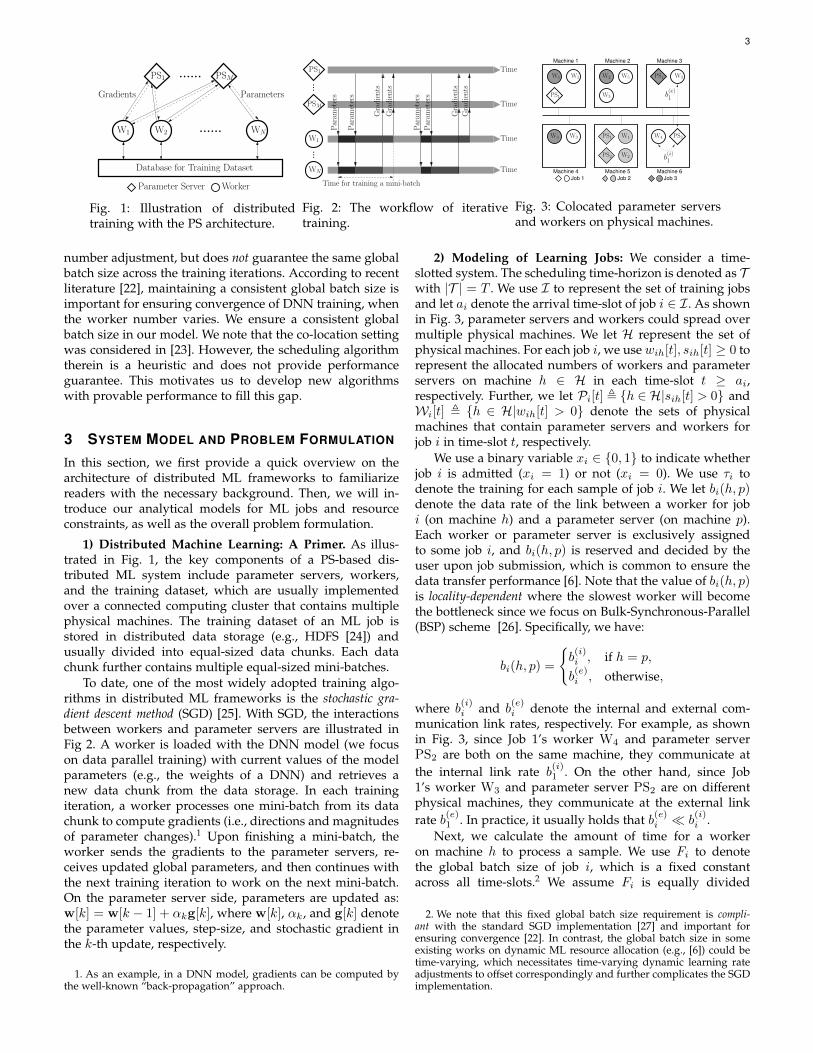
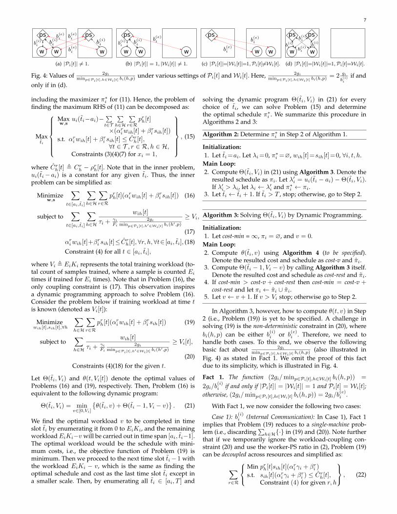
In Algorithm 3, however, how to compute θ(t, v) in Step2 (i.e., Problem (19)) is yet to be specified. A challenge insolving (19) is the non-deterministic constraint in (20), wherebi(h, p) can be either b(i)i or b(e)i . Therefore, we need tohandle both cases. To this end, we observe the followingbasic fact about 2gi

minp∈Pi[t],h∈Wi[t] bi(h,p)(also illustrated in

Fig. 4) as stated in Fact 1. We omit the proof of this factdue to its simplicity, which is illustrated in Fig. 4.

Fact 1. The function (2gi/minp∈Pi[t],h∈Wi[t] bi(h, p)) =

2gi/b(i)i if and only if |Pi[t]| = |Wi[t]| = 1 and Pi[t] = Wi[t];

otherwise, (2gi/minp∈Pi[t],h∈Wi[t] bi(h, p)) = 2gi/b(e)i .

With Fact 1, we now consider the following two cases:

Case 1): b(i)i (Internal Communication): In Case 1), Fact 1implies that Problem (19) reduces to a single-machine prob-lem (i.e., discarding

∑h∈H{·} in (19) and (20)). Note further

that if we temporarily ignore the workload-coupling con-straint (20) and use the worker-PS ratio in (2), Problem (19)can be decoupled across resources and simplified as:

∑r∈R

Min prh[t]sih[t](αri γi + βri )

s.t. sih[t](αri γi + βri ) ≤ Crh[t],Constraint (4) for given r, h

, (22)

8

where each summand in (22) is an integer linear program(ILP) having a trivial solution wih[t] = sih[t] = 0, ∀h ∈ H.However, wih[t] = 0, ∀h ∈ H, clearly violates the workloadconstraint (20). Thus, when (22) is optimal, there should beexactly one machine h′ ∈ H with wih′ [t] ≥ 1 and exactlyone machine h′′ ∈ H with sih′′ [t] ≥ 1. This observationshows that the optimal solution of (19) tends to favor |Pi[t]| =|Wi[t]| = 1 if the workload constraint (20) is not binding.

Notice that the workload constraint (20) in Case 1) be-comes γisih[t] ≥ Vi[t](τi+ 2giγi

b(i)i Fi

). This implies the following

simple solution: We can first sort each physical machineh according to

∑r∈R p

rh[t](αri γi + βri ) and calculate the

minimum number of sih[t] = Vi[t](τi + 2giγi

b(i)i Fi

)/γi from the

workload constraint. The last step is to check if the machinesatisfy the resource capacity constraint (18) and constraint(4). If so, we return the schedule (wih[t], sih[t]) and thecorresponding cost value.

Case 2): b(e)i (External Communication): For those settingsthat do not satisfy |Pi[t]| = |Wi[t]| = 1 and Pi[t] = Wi[t],Fact 1 indicates that parameter servers and workers are com-municating at external rate b(e)i . In this case, the workloadconstraint (20) simply becomes:

∑h∈H wih[t] ≥ Vi[t](τi +

2giγi

b(e)i Fi

). Then, we can rewrite Problem (19) as:

Minimizewih[t],sih[t],∀h

∑h∈H

pwh [t]wih[t] + psh[t]sih[t] (23)

subject to αriwih[t] + βri sih[t] ≤ Crh[t], ∀h, r, (24)∑h∈H

wih[t] ≤ Fi, (25)∑h∈H

wih[t] ≥ Vi[t](τi +

2giγi

b(e)i Fi

), (26)

where pwh [t] ,∑r∈R p

rh[t]αri and psh[t] ,

∑r∈R p

rh[t]βri

denote the aggregated prices of all resources of allocatingworkers and PSs on machine h in time t, respectively.

Unfortunately, Problem (23) is a highly challenging in-teger programming problem with generalized packing andcover type constraints (i.e., integer variables rather than 0-1 variables) in (24)–(26), respectively, which is clearly NP-Hard. Also, it is well-known that there are no polynomialtime approximation schemes (PTAS) even for the basic set-cover and bin-packing problems unless P = NP [31]. In whatfollows, we will pursue an instance-dependent constantratio approximation scheme to solve Problem (23) in thispaper. To this end, we propose a randomized roundingscheme: First, we solve the linear programming relaxationof Problem (23). Let {wih[t], sih[t],∀h, t} be the fractionaloptimal solution. We let δ ∈ (0, 1] be a parameter. LetGδ be a constant (the notation Gδ signifies that Gδ isdependent on δ) to be defined later, and let w′ih[t] =Gδwih[t], s′ih[t] =Gδ sih[t], ∀h, t. Then, we randomly round{w′ih[t], s′ih[t],∀h, t} to obtain an integer solution as follows:

wih[t] =

{dw′ih[t]e, with probability w′ih[t]− bw′ih[t]c,bw′ih[t]c, with probability dw′ih[t]e − w′ih[t],

(27)

sih[t] =

{ds′ih[t]e, with probability s′ih[t]− bs′ih[t]c,bs′ih[t]c, with probability ds′ih[t]e − s′ih[t].

(28)

We will later prove in Theorem 3 (when 0 < Gδ ≤ 1) andTheorem 4 (when Gδ > 1) that the approximation ratio of

this randomized rounding scheme in (27)-(28) enjoys a ratiothat is independent on the problem size.

Lastly, summarizing results in Cases 1) – 2) yields the fol-lowing approximation algorithm for solving Problem (19):

Algorithm 4: Solving θ(t, v) (i.e., Problem (19)).

Initialization:1. Let wih[t]=sih[t]=0, ∀h. Let h=1. Pick some δ ∈ (0, 1].

Let Gδ be defined as in Eq. (29) or Eqn (30). Let D =

dv(τi + 2giγi/(b(i)i Fi))e. Let h∗ = ∅. Let cost-min= ∞.

Choose some integer S ≥ 1. Let iter ← 1.Handling Internal Communication:2. Sort machines in H according to

∑r∈R p

rh[t](αri γi + βri )

in non-decreasing order into h1, h2, ..., hH .3. Calculate the minimum number of sih[t] = Vi[t]

(τi +

2giγi

b(i)i Fi

)/γi.

4. If Constraint (4) is not satisfied, go to Step 7.5. If Constraint (24) is not satisfied, go to Step 7.6. Return cost-min

∑r∈R p

rh[t]sih[t](αri γi + βri ) and h∗ = h.

7. Let h← h+ 1. If h > H , stop; otherwise, go to Step 2.Handling External Communication:8. Solve the linear programming relaxation of Problem (23).

Let {wih[t], sih[t],∀h, t} be the fractional optimal solu-tion.

9. Let w′ih[t] = Gδwih[t], s′ih[t] = Gδ sih[t], ∀h, t.10. Generate an integer solution {wih[t], sih[t],∀h, t} follow-

ing the randomized rounding scheme in (27)–(28).11. If {wih[t], sih[t],∀h, t} is infeasible or iter < S, then

iter ← iter + 1, go to Step 10.Final Step:12. Compare the solutions between internal and external

cases. Pick the one with the lowest cost among themand return the cost and the corresponding schedule{wih[t], sih[t],∀h, t}.

In the internal communication part of Algorithm 4, wefirst sort the machines and then check each machine one byone (Step 2). We calculate the minimum number of sih[t]needed to satisfy the learning workload demand D (Step3). If Constraint (4) is satisfied (Step 4), we further checkthe resource capacity constraint (18) (Step 5). If we detect amachine with all above constraints satisfied, we return thecost and schedule accordingly (Step 6). After exploring onemachine, we move on to the next one as long as it is not thelast machine (Step 7). The external communication part isbased on LP relaxation (Step 8) and randomized rounding(Step 9-12). Note that the randomized rounding will findat most S integer feasible solutions (Step 12). Finally, wechoose the lowest cost among the solutions from the internaland external communication parts (Step 13).

4.4 Theoretical Performance AnalysisWe now examine the competitive ratio of our PD-ORSalgorithm. Note that the key component in PD-ORS is ourproposed randomized rounding scheme in (27)–(28), whichis in turn the foundation of Algorithm 1. Thus, we first provethe following results regarding the randomized roundingalgorithm. Consider an integer program with generalizedcover/packing constraints: min{c>x : Ax ≥ a,Bx ≤

9

0.02 0.04 0.06 0.08 0.1

The value of

0

0.02

0.04

0.06

0.08

0.1

The v

alu

e o

f R

HS

Wa=30 =RHS

Wa=40

Wa=35

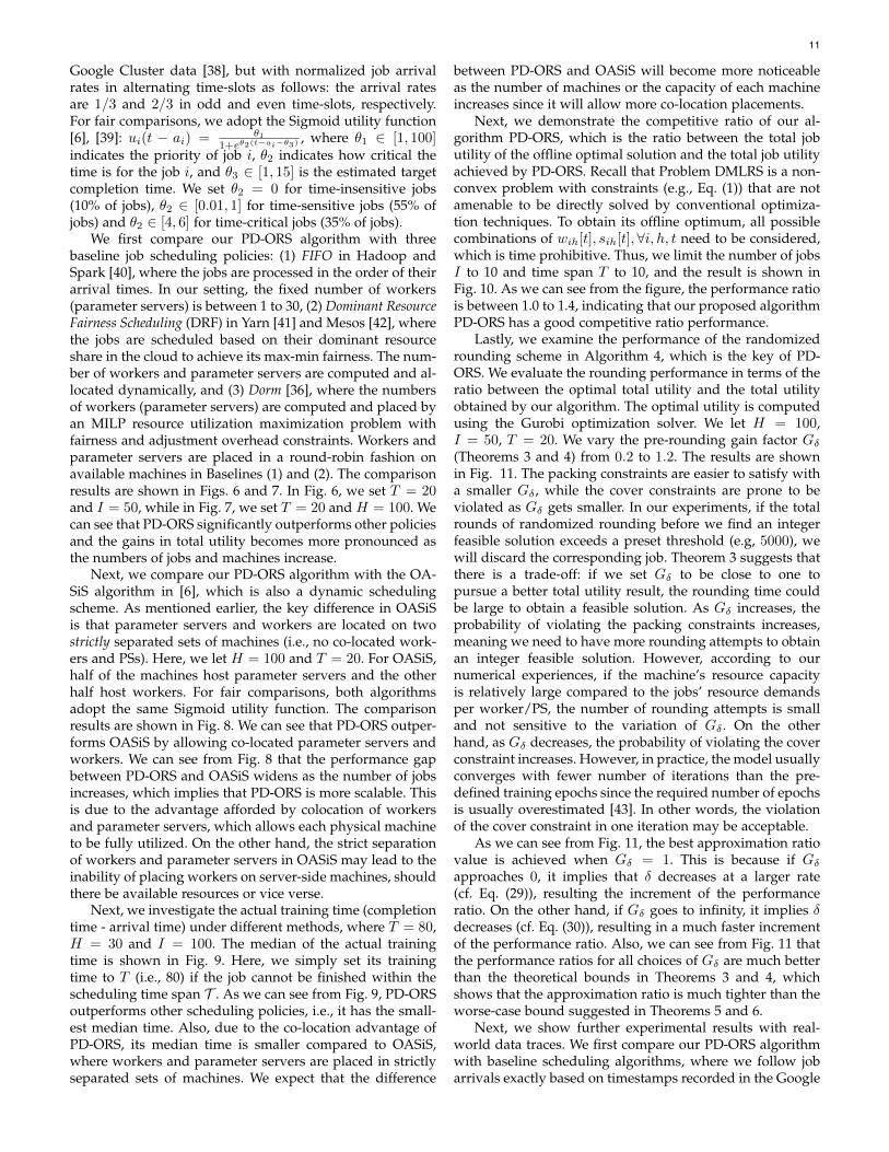
Fig. 5: The feasibility study.

b,x ∈ Zn+}, where A ∈ Rm×n+ , B ∈ Rr×n+ , a ∈ Rm+ ,b ∈ Rr+, and c ∈ Rn+. Let x be a fractional optimal solution.Consider the randomized rounding scheme: Let x′ = Gδxfor some Gδ (to be specified). Randomly round x′ to x ∈ Zn+as: xj = dx′je w.p. x′j − bx′jc and xj = bx′jc o.w. Notethat in the rounding process, if Gδ > 1 (Gδ ∈ (0, 1]), thepacking (cover) constraint is prone to be violated and thecover (packing) constraint is easier to be satisfied. Hence,depending on which constraint is more preferred to befeasible, we consider two cases with respect to Gδ .

1) 0 < Gδ ≤ 1: We have the following approximationresult (see proof in Appendix A):

Lemma 1 (Rounding). Let Wa,min{ai/[A]ij : [A]ij>0} andWb,min{bi/[B]ij : [B]ij>0}. Let δ ∈ (0, 1] be a given constantand define Gδ as:

Gδ , 1 +3 ln(3r/δ)

2Wb−

√(3 ln(3r/δ)

2Wb

)2

+3 ln(3r/δ)

Wb.

Then, with probability greater than 1−δ, x achieves a cost at most3Gδδ times the cost of x. Meanwhile, x satisfies Pr

{(Ax)i ≤

ai(1− ( 2GδWa

ln( 3mδ ))

12 )Gδ,∃i

}≤ δ

3m .

Remark 1 (Discussions on Feasibility). An insightful remarkof Lemma 1 is in order. Note that, theoretically, the expres-sion 1 − ( 2

GδWaln( 3m

δ ))12 in Lemma 1 could become nega-

tive. In this case, the last probabilistic inequality in Lemma 1trivially holds and is not meaningful in characterizing thefeasibility, even though the inequality remains valid. Inorder for the probabilistic statement to be meaningful incharacterizing the feasibility of the integer linear program,we solve for δ by enforcing 1− ( 2

GδWaln( 3m

δ ))12 > 0, which

yields δ ≥ 3m/eGδWa

2 . On the other hand, we prefer δ tobe small since it bounds the feasibility violation probabilityand approximation ratio achievability in Lemma 1. Hence,the smaller the value of 3m/e

GδWa2 , the less restrictive the

condition δ ≥ 3m/eGδWa

2 is.To gain a deeper understanding on how restrictive the

condition δ ≥ 3m/eGδWa

2 is, we conduct a case studyand the results are illustrated in Fig. 5. Here, we let RHS, 3m/e

GδWa2 for convenience. We vary δ from 0.02 to 0.1.

Clearly, the left-hand-side (LHS) of the condition is the 45◦

straight line. In order for the condition to hold, the curve ofRHS should fall under this straight line. Based on typicalcomputing cluster parameters, we set Wb to 15, and setr , RH+1 to 401 (R = 4, H = 100). We can see from Fig. 5that as Wa increases, the curve of RHS crosses the dashedline of LHS at a smaller δ-value. This means that, the largerthe value ofWa, the easier for 1−( 2

GδWaln( 3m

δ ))12 to become

positive. Hence, the probabilistic feasibility characterizationin Lemma 1 is useful for typical system parameters inpractice.

2) Gδ > 1: We have the following approximation result(see proof in Appendix B):

Lemma 2 (Rounding). Let Wa , min{ai/[A]ij : [A]ij > 0}and Wb , min{bi/[B]ij : [B]ij > 0}. Let δ ∈ (0, 1] be a givenconstant and define Gδ as:

Gδ , 1 +ln(3m/δ)

Wa+

√(ln(3m/δ)

Wa

)2

+2 ln(3m/δ)

Wa.

Then, with probability greater than 1 − δ, x achieves a cost atmost 3Gδ

δ times the cost of x. Meanwhile, x satisfies Pr{

(Bx)i >

bi(1 + ( 3GδWb

ln( 3rδ ))

12 )Gδ,∃i

}≤ δ

3r .

Several important remarks for Lemmas 1 and 2 aresummarized as follows:i) Note that Alg. 4 is a randomized algorithm. Therefore,its performance is also characterized probabilistically, andδ is used for such probabilistic characterization. Here, itmeans that with probability 1−δ, one achieves an approx-imation ratio at most 3Gδ

δ and a probabilistic feasibilityguarantee as stated in Lemma 1 when 0 < Gδ ≤ 1 andLemma 2 when Gδ > 1. In other words, the statementsmean that the probability of getting a better approxi-mation ratio is smaller under randomized rounding (i.e.,better approximation ratio ⇒ smaller 3Gδ

δ ⇒ larger δ ⇒smaller probability 1 − δ). That is, the trade-off betweenthe approximation ratio value and its achieving probabil-ity is quantified by δ. A larger δ implies a smaller approx-imation ratio, but the probability of obtaining a feasiblesolution of this ratio is also smaller (i.e., more rounds ofrounding needed). Interestingly, for δ = 1, Lemmas 1 and2 indicate that there is still non-zero probability to achievean approximation ratio not exceeding 3Gδ .

ii) Note that if we pickGδ ∈ (0, 1], the approximation ratio3Gδδ decreases (the smaller the approximation ratio, the

better) as δ increases based on Eqn. (35) in Appendix A.However, the growth rate of Gδ is slower compared tothat of δ due to the log operator. On the other hand, ifwe pick Gδ > 1, 3Gδ

δ decreases as δ increases accordingto Eqn. (38) in Appendix B. Therefore, the approximationratio is ultimately controlled by parameter δ. Also, thetheoretical approximation ratio 3Gδ

δ is conservative. Ournumerical studies show that the approximation ratio per-formance in reality is much smaller than 3Gδ

δ .iii) The probabilistic guarantee of the cover constraint(Ax ≥ a) when 0 < Gδ ≤ 1 and packing constraint(Bx ≤ b) when Gδ > 1, is unavoidable and due tothe fundamental hardness of satisfying both cover and

10

packing constraints, which are of conflicting nature: Anystrategy trying to better satisfy the packing constraints(multiplying a Gδ-factor with Gδ ∈ (0, 1]) may increasethe probability of violating the cover constraints, and theprobability of violating the packing constraints may beincreased otherwise. However, the probabilistic boundhere is for worst case and may be pessimistic.

iv) The results in Lemmas 1 and 2 are in fact applicablefor general ILP with mixed cover/packing constraints.Hence, the results and their insights in Lemmas 1 and2 could be of independent theoretical interest.By specializing Lemma 1 and Lemma 2 with parameters

in Problem (23), we have the following approximation re-sults for Algorithm 4. The first result corresponds to the casewhere the feasibility of the resource constraint (packing) ismore favored, i.e., 0 < Gδ ≤ 1:

Theorem 3 (Approximation Performance of Alg. 4 WhenResource Constraint Feasibility is Favored). Let W1 ,Vi[t]

(τi + 2giγi

b(e)i Fi

), W2 , min{Fi, Crh[t]/αri , C

rh[t]/βri ,∀r, h},

and δ ∈ (0, 1]. Define Gδ as:

Gδ,1+3 ln(3(RH+1)/δ)

2W2

−

√(3 ln(3(RH + 1)/δ)

2W2

)2

+3 ln(3(RH+1)/δ)

W2. (29)

Then, with probability greater than 1 − δ, Algorithm 4 ob-tains a schedule {wih[t], sih[t],∀t, h} that has an approx-imation ratio at most 3Gδ

δ with Pr{LHS(26) ≤ W1(1 −( 2GδW1

ln( 3δ ))

12 )Gδ,∃i} ≤ δ

3 .

The next result corresponds to the case where the fea-sibility of the workload constraint (cover) is more favored,i.e., Gδ > 1:

Theorem 4 (Approximation Performance of Alg. 4 WhenWorkload Constraint Feasibility is Favored). Let W1 ,Vi[t]

(τi + 2giγi

b(e)i Fi

), W2 , min{Fi, Crh[t]/αri , C

rh[t]/βri ,∀r, h},

and δ ∈ (0, 1]. Define Gδ as:

Gδ , 1 +ln(3/δ)

W1+

√(ln(3/δ)

W1

)2

+2 ln(3/δ)

W1. (30)

Then, with probability greater than 1 − δ, Algorithm 4 ob-tains a schedule {wih[t], sih[t],∀t, h} that has an approxima-tion ratio at most 3Gδ

δ with Pr{LHS(24) > Crh[t]Gδ(1 +

( 3GδW2

ln( 3(HR+1)δ ))

12 )} ≤ δ

3(HR+1) .

Note that Eqn. (25) is guaranteed in practice since thenumber of samples is typically far more than the numberof workers. The competitive ratio of our online algorithmis the worst-case upper bound of the ratio of the overallutility of admitted jobs devided by the offline optimalsolution of Problem DMLRS to the total utility of admittedjobs achieved by Algorithm 1 in the overall time horizon.Theorems 3 and 4 follow directly from Lemmas 1 and 2,respectively, and we omit the proof here for brevity. Basedon these results, we can establish the overall competitiveratio for Algorithm 1 as follows.

Theorem 5 (Competitive Ratio of Alg 1 when 0<Gδ ≤ 1).Let δ, Gδ and W1 be as defined in Theorem 3. Let Ur and L

be as defined in (13) and (14), respectively. Then, with probabilitygreater than (1−(δ/3)S)TKiEi , PD-ORS in Algorithm 1 returnsa feasible solution that is 6Gδ

δ maxr∈R(1, ln Ur

L )–competitive.

Theorem 6 (Competitive Ratio of Alg 1 whenGδ > 1). Let δ,Gδ andW2 be as defined in Theorem 4. Let Ur and L be as definedin (13) and (14), respectively. Then, with probability greater than(1− (δ/3(HR+ 1))S)TKiEi , PD-ORS in Algorithm 1 returnsa feasible solution that is 6Gδ

δ maxr∈R(1, ln Ur

L )–competitive.

It is worth pointing out that in Theorems 5 and 6, the fea-sibility achieving probability values, i.e., (1− (δ/3)S)TKiEi

and (1− (δ/3(HR+1))S)TKiEi , can controlled by choosingappropriate values of δ and S (i.e., rounds of rounding) tooffset the impact of total number of DP iterations TKiEi.The smaller δ and the larger S are, the higher the feasibilityachieving probability. Theorems 5 and 6 can be proved byweak duality and the approximation results in Theorems 3and 4. We provide a proof in Appendix C.

Theorem 7 (Polynomial Running Time). By combin-ing Algorithms 1–4, the time complexity of PD-ORS isO(∑|I|i=1 TK

2i E

2i (H3 + S)), which is polynomial.

Proof. When solving θ(t, v) using Algorithm 4, it takesO(H logH) iterations to sort machines in internal commu-nication case under each time slot t and looping all machinesto calculate the minimum number sih[t] takes O(H). Thus,it takes (H logH) time for the internal communication partin Algorithm 4. For the external communication part inAlgorithm 4, solving the LP relaxation of Problem (23) canbe approximately bounded O(H3) if we use a polynomialtime LP solver (e.g., Vaidya’s algorithm [33]). Accordingto Algorithm 4, the rounding time is proportional to S.Hence, the running time for the external communicationspart is upper bounded by O(|H|3 + S). Combining thediscussions above, the running time complexity of Algo-rithm 4 is O(H logH + H3 + S) = O(H3 + S). Moreover,the number of states (t, v) is O(TKiEi) in the dynamicprogramming (DP) for each job i, and the time complexityof executing DP is O(KiEi). Thus, the time complexity isO(TK2

i E2i ) in DP. In Algorithm 1, the number of steps in

the main loop is equal to the number of jobs. Therefore,the overall running time complexity can be computed asO(∑|I|i=1 TK

2i E

2i (H3 + S)).

5 NUMERICAL RESULTS

In this section, we conduct simulation studies to evaluatethe efficacy of our proposed PD-ORS algorithm. We testan ML system with jobs parameters generated uniformlyat random from the following intervals: Ei ∈ [50, 200],Ki ∈ [20000, 500000], gi ∈ [30, 575] MB, τi ∈ [10−5, 10−4]time slots, γi ∈ [1, 10], Fi ∈ [1, 200]. We consider fourtypes of resources: GPU, CPU, memory, and storage. For faircomparisons, following similar settings in [34] [35] [36], weset resource demand of each worker as follows: 0–4 GPUs,1–10 vCPUs, 2–32 GB memory, and 5–10GB storage. We setresource demand of each parameter server as follows: 1–10vCPUs, 2–32GB memory and 5-10GB storage. The resourcecapacity of each physical machine is set roughly 18 times ofthe resource demands of a worker/PS following EC2 C5ninstances [37]. We set the job arrival pattern according to the

11

Google Cluster data [38], but with normalized job arrivalrates in alternating time-slots as follows: the arrival ratesare 1/3 and 2/3 in odd and even time-slots, respectively.For fair comparisons, we adopt the Sigmoid utility function[6], [39]: ui(t − ai) = θ1

1+eθ2(t−ai−θ3) , where θ1 ∈ [1, 100]indicates the priority of job i, θ2 indicates how critical thetime is for the job i, and θ3 ∈ [1, 15] is the estimated targetcompletion time. We set θ2 = 0 for time-insensitive jobs(10% of jobs), θ2 ∈ [0.01, 1] for time-sensitive jobs (55% ofjobs) and θ2 ∈ [4, 6] for time-critical jobs (35% of jobs).

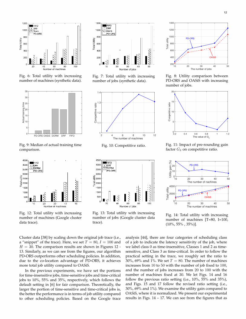
We first compare our PD-ORS algorithm with threebaseline job scheduling policies: (1) FIFO in Hadoop andSpark [40], where the jobs are processed in the order of theirarrival times. In our setting, the fixed number of workers(parameter servers) is between 1 to 30, (2) Dominant ResourceFairness Scheduling (DRF) in Yarn [41] and Mesos [42], wherethe jobs are scheduled based on their dominant resourceshare in the cloud to achieve its max-min fairness. The num-ber of workers and parameter servers are computed and al-located dynamically, and (3) Dorm [36], where the numbersof workers (parameter servers) are computed and placed byan MILP resource utilization maximization problem withfairness and adjustment overhead constraints. Workers andparameter servers are placed in a round-robin fashion onavailable machines in Baselines (1) and (2). The comparisonresults are shown in Figs. 6 and 7. In Fig. 6, we set T = 20and I = 50, while in Fig. 7, we set T = 20 and H = 100. Wecan see that PD-ORS significantly outperforms other policiesand the gains in total utility becomes more pronounced asthe numbers of jobs and machines increase.

Next, we compare our PD-ORS algorithm with the OA-SiS algorithm in [6], which is also a dynamic schedulingscheme. As mentioned earlier, the key difference in OASiSis that parameter servers and workers are located on twostrictly separated sets of machines (i.e., no co-located work-ers and PSs). Here, we let H = 100 and T = 20. For OASiS,half of the machines host parameter servers and the otherhalf host workers. For fair comparisons, both algorithmsadopt the same Sigmoid utility function. The comparisonresults are shown in Fig. 8. We can see that PD-ORS outper-forms OASiS by allowing co-located parameter servers andworkers. We can see from Fig. 8 that the performance gapbetween PD-ORS and OASiS widens as the number of jobsincreases, which implies that PD-ORS is more scalable. Thisis due to the advantage afforded by colocation of workersand parameter servers, which allows each physical machineto be fully utilized. On the other hand, the strict separationof workers and parameter servers in OASiS may lead to theinability of placing workers on server-side machines, shouldthere be available resources or vice verse.

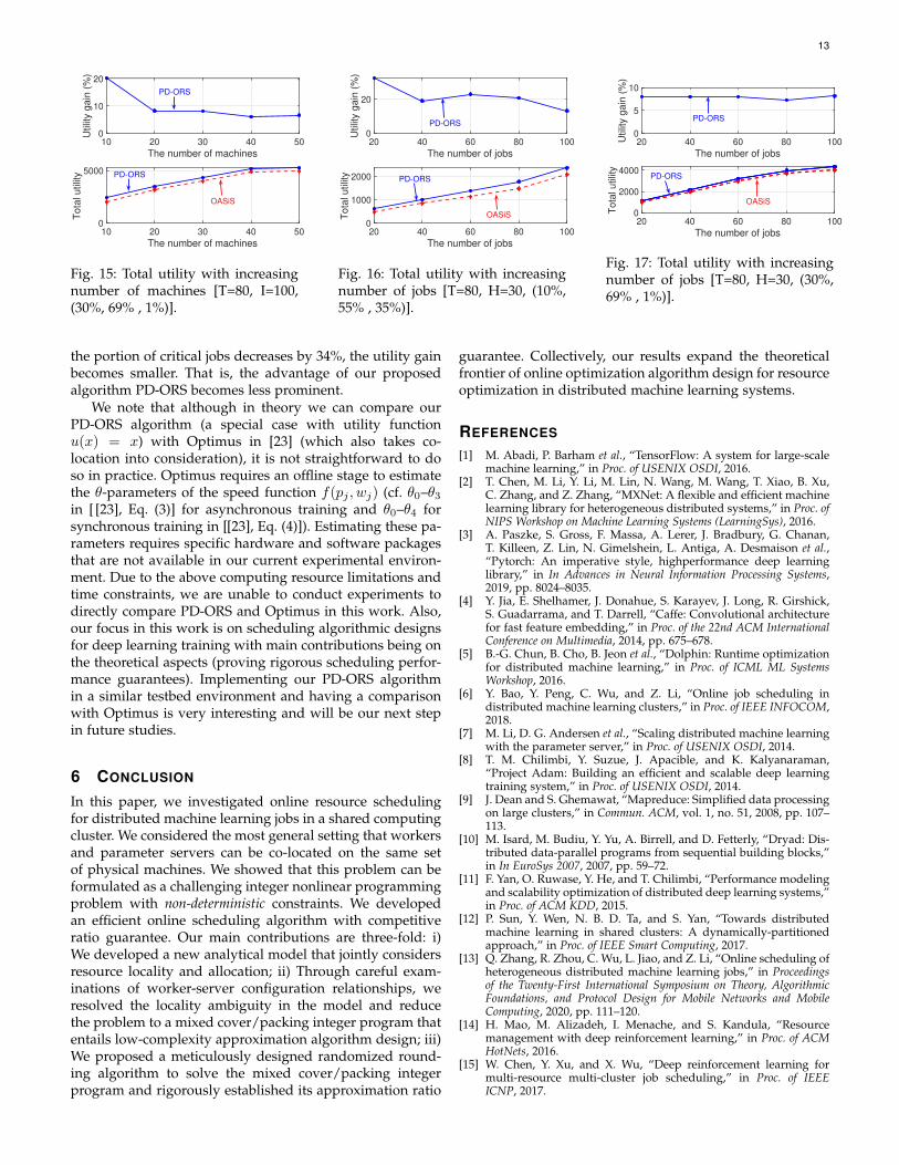
Next, we investigate the actual training time (completiontime - arrival time) under different methods, where T = 80,H = 30 and I = 100. The median of the actual trainingtime is shown in Fig. 9. Here, we simply set its trainingtime to T (i.e., 80) if the job cannot be finished within thescheduling time span T . As we can see from Fig. 9, PD-ORSoutperforms other scheduling policies, i.e., it has the small-est median time. Also, due to the co-location advantage ofPD-ORS, its median time is smaller compared to OASiS,where workers and parameter servers are placed in strictlyseparated sets of machines. We expect that the difference

between PD-ORS and OASiS will become more noticeableas the number of machines or the capacity of each machineincreases since it will allow more co-location placements.

Next, we demonstrate the competitive ratio of our al-gorithm PD-ORS, which is the ratio between the total jobutility of the offline optimal solution and the total job utilityachieved by PD-ORS. Recall that Problem DMLRS is a non-convex problem with constraints (e.g., Eq. (1)) that are notamenable to be directly solved by conventional optimiza-tion techniques. To obtain its offline optimum, all possiblecombinations of wih[t], sih[t],∀i, h, t need to be considered,which is time prohibitive. Thus, we limit the number of jobsI to 10 and time span T to 10, and the result is shown inFig. 10. As we can see from the figure, the performance ratiois between 1.0 to 1.4, indicating that our proposed algorithmPD-ORS has a good competitive ratio performance.

Lastly, we examine the performance of the randomizedrounding scheme in Algorithm 4, which is the key of PD-ORS. We evaluate the rounding performance in terms of theratio between the optimal total utility and the total utilityobtained by our algorithm. The optimal utility is computedusing the Gurobi optimization solver. We let H = 100,I = 50, T = 20. We vary the pre-rounding gain factor Gδ(Theorems 3 and 4) from 0.2 to 1.2. The results are shownin Fig. 11. The packing constraints are easier to satisfy witha smaller Gδ , while the cover constraints are prone to beviolated as Gδ gets smaller. In our experiments, if the totalrounds of randomized rounding before we find an integerfeasible solution exceeds a preset threshold (e.g, 5000), wewill discard the corresponding job. Theorem 3 suggests thatthere is a trade-off: if we set Gδ to be close to one topursue a better total utility result, the rounding time couldbe large to obtain a feasible solution. As Gδ increases, theprobability of violating the packing constraints increases,meaning we need to have more rounding attempts to obtainan integer feasible solution. However, according to ournumerical experiences, if the machine’s resource capacityis relatively large compared to the jobs’ resource demandsper worker/PS, the number of rounding attempts is smalland not sensitive to the variation of Gδ . On the otherhand, as Gδ decreases, the probability of violating the coverconstraint increases. However, in practice, the model usuallyconverges with fewer number of iterations than the pre-defined training epochs since the required number of epochsis usually overestimated [43]. In other words, the violationof the cover constraint in one iteration may be acceptable.

As we can see from Fig. 11, the best approximation ratiovalue is achieved when Gδ = 1. This is because if Gδapproaches 0, it implies that δ decreases at a larger rate(cf. Eq. (29)), resulting the increment of the performanceratio. On the other hand, if Gδ goes to infinity, it implies δdecreases (cf. Eq. (30)), resulting in a much faster incrementof the performance ratio. Also, we can see from Fig. 11 thatthe performance ratios for all choices of Gδ are much betterthan the theoretical bounds in Theorems 3 and 4, whichshows that the approximation ratio is much tighter than theworse-case bound suggested in Theorems 5 and 6.

Next, we show further experimental results with real-world data traces. We first compare our PD-ORS algorithmwith baseline scheduling algorithms, where we follow jobarrivals exactly based on timestamps recorded in the Google

12

Fig. 6: Total utility with increasingnumber of machines (synthetic data).

Fig. 7: Total utility with increasingnumber of jobs (synthetic data).

10 20 30 40 50

The number of jobs

200

400

600

800

1000

1200

1400

Tota

l utilit

y PD-ORS

OASiS

Fig. 8: Utility comparison betweenPD-ORS and OASiS with increasingnumber of jobs.

PD-ORS OASiS DORM DRF FIFO0

5

10

15

20

25

30

35

Actu

al tr

ain

ing tim

e

Fig. 9: Median of actual training timecomparison.

2 4 6 8 10 12

The number of machines

1

1.1

1.2

1.3

1.4

Com

petitive r

atio

Fig. 10: Competitive ratio.

0.2 0.4 0.6 0.8 1 1.2

The value of G

0

5

10

15

20

Com

pet

itiv

e ra

tio

Fig. 11: Impact of pre-rounding gainfactor Gδ on competitive ratio.

Fig. 12: Total utility with increasingnumber of machines (Google clusterdata trace).

Fig. 13: Total utility with increasingnumber of jobs (Google cluster datatrace).

10 20 30 40 50

The number of nachines

0

10

20

Utilit

y g

ain

(%

)

10 20 30 40 50

The number of machines

0

2000

4000

To

tal u

tilit

yPD-ORS

PD-ORS

OASiS

Fig. 14: Total utility with increasingnumber of machines [T=80, I=100,(10%, 55% , 35%)].

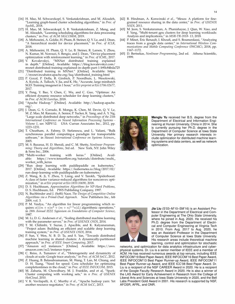
Cluster data [38] by scaling down the original job trace (i.e.,a “snippet” of the trace). Here, we set T = 80, I = 100 andH = 30. The comparison results are shown in Figures 12 -13. Similarly, as we can see from the figures, our algorithmPD-ORS outperforms other scheduling policies. In addition,due to the co-location advantage of PD-ORS, it achievesmore total job utility compared to OASiS.

In the previous experiments, we have set the portionsfor time-insensitive jobs, time-sensitive jobs and time-criticaljobs to 10%, 55% and 35%, respectively, which follows thedefault setting in [6] for fair comparison. Theoretically, thelarger the portion of time-sensitive and time-critical jobs is,the better the performance is in terms of job utility comparedto other scheduling policies. Based on the Google trace

analysis [44], there are four categories of scheduling classof a job to indicate the latency sensitivity of the job, wherewe label class 0 as time-insensitive, Classes 1 and 2 as time-sensitive, and Class 3 as time-critical. In order to follow thepractical setting in the trace, we roughly set the ratio to30%, 69% and 1%. We set T = 80. The number of machinesincreases from 10 to 50 with the number of job fixed to 100,and the number of jobs increases from 20 to 100 with thenumber of machines fixed at 30. We let Figs. 14 and 16follow the previous ratio setting (i.e., 10%, 55% and 35%),and Figs. 15 and 17 follow the revised ratio setting (i.e.,30%, 69% and 1%). We examine the utility gain compared toOASiS, where it is normalized. We present our experimentalresults in Figs. 14 – 17. We can see from the figures that as

13

10 20 30 40 50

The number of machines

0

10

20U

tilit

y g

ain

(%

)

10 20 30 40 50

The number of machines

0

5000

To

tal u

tilit

y

PD-ORS

PD-ORS

OASiS

Fig. 15: Total utility with increasingnumber of machines [T=80, I=100,(30%, 69% , 1%)].

20 40 60 80 100

The number of jobs

0

20

Utilit

y g

ain

(%

)

20 40 60 80 100

The number of jobs

0

1000

2000

To

tal u

tilit

y

PD-ORS

PD-ORS

OASiS

Fig. 16: Total utility with increasingnumber of jobs [T=80, H=30, (10%,55% , 35%)].

20 40 60 80 100

The number of jobs

0

5

10

Utilit

y g

ain

(%

)

20 40 60 80 100

The number of jobs

0

2000

4000

To

tal u

tilit

y

PD-ORS

PD-ORS

OASiS

Fig. 17: Total utility with increasingnumber of jobs [T=80, H=30, (30%,69% , 1%)].

the portion of critical jobs decreases by 34%, the utility gainbecomes smaller. That is, the advantage of our proposedalgorithm PD-ORS becomes less prominent.

We note that although in theory we can compare ourPD-ORS algorithm (a special case with utility functionu(x) = x) with Optimus in [23] (which also takes co-location into consideration), it is not straightforward to doso in practice. Optimus requires an offline stage to estimatethe θ-parameters of the speed function f(pj , wj) (cf. θ0–θ3

in [ [23], Eq. (3)] for asynchronous training and θ0–θ4 forsynchronous training in [[23], Eq. (4)]). Estimating these pa-rameters requires specific hardware and software packagesthat are not available in our current experimental environ-ment. Due to the above computing resource limitations andtime constraints, we are unable to conduct experiments todirectly compare PD-ORS and Optimus in this work. Also,our focus in this work is on scheduling algorithmic designsfor deep learning training with main contributions being onthe theoretical aspects (proving rigorous scheduling perfor-mance guarantees). Implementing our PD-ORS algorithmin a similar testbed environment and having a comparisonwith Optimus is very interesting and will be our next stepin future studies.

6 CONCLUSION

In this paper, we investigated online resource schedulingfor distributed machine learning jobs in a shared computingcluster. We considered the most general setting that workersand parameter servers can be co-located on the same setof physical machines. We showed that this problem can beformulated as a challenging integer nonlinear programmingproblem with non-deterministic constraints. We developedan efficient online scheduling algorithm with competitiveratio guarantee. Our main contributions are three-fold: i)We developed a new analytical model that jointly considersresource locality and allocation; ii) Through careful exam-inations of worker-server configuration relationships, weresolved the locality ambiguity in the model and reducethe problem to a mixed cover/packing integer program thatentails low-complexity approximation algorithm design; iii)We proposed a meticulously designed randomized round-ing algorithm to solve the mixed cover/packing integerprogram and rigorously established its approximation ratio

guarantee. Collectively, our results expand the theoreticalfrontier of online optimization algorithm design for resourceoptimization in distributed machine learning systems.

REFERENCES

[1] M. Abadi, P. Barham et al., “TensorFlow: A system for large-scalemachine learning,” in Proc. of USENIX OSDI, 2016.

[2] T. Chen, M. Li, Y. Li, M. Lin, N. Wang, M. Wang, T. Xiao, B. Xu,C. Zhang, and Z. Zhang, “MXNet: A flexible and efficient machinelearning library for heterogeneous distributed systems,” in Proc. ofNIPS Workshop on Machine Learning Systems (LearningSys), 2016.

[3] A. Paszke, S. Gross, F. Massa, A. Lerer, J. Bradbury, G. Chanan,T. Killeen, Z. Lin, N. Gimelshein, L. Antiga, A. Desmaison et al.,“Pytorch: An imperative style, highperformance deep learninglibrary,” in In Advances in Neural Information Processing Systems,2019, pp. 8024–8035.

[4] Y. Jia, E. Shelhamer, J. Donahue, S. Karayev, J. Long, R. Girshick,S. Guadarrama, and T. Darrell, “Caffe: Convolutional architecturefor fast feature embedding,” in Proc. of the 22nd ACM InternationalConference on Multimedia, 2014, pp. 675–678.

[5] B.-G. Chun, B. Cho, B. Jeon et al., “Dolphin: Runtime optimizationfor distributed machine learning,” in Proc. of ICML ML SystemsWorkshop, 2016.

[6] Y. Bao, Y. Peng, C. Wu, and Z. Li, “Online job scheduling indistributed machine learning clusters,” in Proc. of IEEE INFOCOM,2018.

[7] M. Li, D. G. Andersen et al., “Scaling distributed machine learningwith the parameter server,” in Proc. of USENIX OSDI, 2014.

[8] T. M. Chilimbi, Y. Suzue, J. Apacible, and K. Kalyanaraman,“Project Adam: Building an efficient and scalable deep learningtraining system,” in Proc. of USENIX OSDI, 2014.

[9] J. Dean and S. Ghemawat, “Mapreduce: Simplified data processingon large clusters,” in Commun. ACM, vol. 1, no. 51, 2008, pp. 107–113.

[10] M. Isard, M. Budiu, Y. Yu, A. Birrell, and D. Fetterly, “Dryad: Dis-tributed data-parallel programs from sequential building blocks,”in In EuroSys 2007, 2007, pp. 59–72.

[11] F. Yan, O. Ruwase, Y. He, and T. Chilimbi, “Performance modelingand scalability optimization of distributed deep learning systems,”in Proc. of ACM KDD, 2015.

[12] P. Sun, Y. Wen, N. B. D. Ta, and S. Yan, “Towards distributedmachine learning in shared clusters: A dynamically-partitionedapproach,” in Proc. of IEEE Smart Computing, 2017.

[13] Q. Zhang, R. Zhou, C. Wu, L. Jiao, and Z. Li, “Online scheduling ofheterogeneous distributed machine learning jobs,” in Proceedingsof the Twenty-First International Symposium on Theory, AlgorithmicFoundations, and Protocol Design for Mobile Networks and MobileComputing, 2020, pp. 111–120.

[14] H. Mao, M. Alizadeh, I. Menache, and S. Kandula, “Resourcemanagement with deep reinforcement learning,” in Proc. of ACMHotNets, 2016.

[15] W. Chen, Y. Xu, and X. Wu, “Deep reinforcement learning formulti-resource multi-cluster job scheduling,” in Proc. of IEEEICNP, 2017.

14

[16] H. Mao, M. Schwarzkopf, S. Venkatakrishnan, and M. Alizadeh,“Learning graph-based cluster scheduling algorithms,” in Proc. ofSysML, 2018.

[17] H. Mao, M. Schwarzkopf, S. B. Venkatakrishnan, Z. Meng, andM. Alizadeh, “Learning scheduling algorithms for data processingclusters,” in Proc. of ACM SIGCOMM, 2019.

[18] A. Mirhoseini, A. Goldie, H. Pham, B. Steiner, Q. V. Le, and J. Dean,“A hierarchical model for device placement,” in Proc. of ICLR,2018.

[19] A. Mirhoseini, H. Pham, Q. V. Le, B. Steiner, R. Larsen, Y. Zhou,N. Kumar, M. Norouzi, S. Bengio, and J. Dean, “Device placementoptimization with reinforcement learning,” in Proc. of ICML, 2017.

[20] V. Kovalevskyi, “MXNet distributed training explainedin depth.” [Online]. Available: https://blog.kovalevskyi.com/mxnet-distributed-training-explained-in-depth-part-1-b90c84bda725

[21] “Distributed training in MXNet.” [Online]. Available: https://mxnet.incubator.apache.org/faq/distributed training.html

[22] P. Goyal, P. Dolla, R. Girshick, P. Noordhuis, L. Wesolowski,A. Kyrola, A. Tulloch, Y. Jia, and K. He, “Accurate, large minibatchSGD: Training imagenet in 1 hour,” arXiv preprint arXiv:1706.02677,2017.

[23] Y. Peng, Y. Bao, Y. Chen, C. Wu, and C. Guo, “Optimus: Anefficient dynamic resource scheduler for deep learning clusters,”in Proc. of ACM EuroSys, 2018.

[24] “Apache Hadoop.” [Online]. Available: http://hadoop.apache.org/.

[25] J. Dean, G. S. Corrado, R. Monga, K. Chen, M. Devin, Q. V. Le,M. Z. Mao, M. Ranzato, A. Senior, P. Tucker, K. Yang, and A. Y. Ng,“Large scale distributed deep networks,” in Proceedings of the 25thInternational Conference on Neural Information Processing Systems -Volume 1, ser. NIPS’12. USA: Curran Associates Inc., 2012, pp.1223–1231.

[26] T. Cheatham, A. Fahmy, D. Siefanescu, and L. Valiani, “Bulksynchronous parallel computing-a paradigm for transportablesoftware,” in Hawaii International Conference on Systems Sciences,,2005.

[27] M. S. Bazaraa, H. D. Sherali, and C. M. Shetty, Nonlinear Program-ming: Theory and Algorithms, 3rd ed. New York, NY: John Wiley& Sons Inc., 2006.

[28] “Multi-worker training with keras.” [Online]. Avail-able: https://www.tensorflow.org/tutorials/distribute/multiworker with keras

[29] “Run deep learning with paddlepaddle on kubernetes,”2017. [Online]. Available: https://kubernetes.io/blog/2017/02/run-deep-learning-with-paddlepaddle-on-kubernetes/

[30] Z. Wang, K. Ji, Y. Zhou, Y. Liang, and V. Tarokh, “Spiderboost:A class of faster variance-reduced algorithms for nonconvex opti-mization,” in arXiv preprint arXiv:1810.10690, 2018.

[31] D. S. Hochbaum, Approximation Algorithms for NP-Hard Problems,D. S. Hochbaum, Ed. PWS Publishing Company, 1997.

[32] N. Buchbinder and J. (Seffi) Naor, The Design of Competitive OnlineAlgorithms via a Primal-Dual Approach. Now Publishers Inc., feb2009, vol. 3.

[33] P. M. Vaidya, “An algorithm for linear programming which re-quires o(((m + n)n2 + (m + n)1.5n)L) algorithmic operations,”in 28th Annual IEEE Syposium on Foundations of Computer Science,1987.

[34] M. Li, D. G. Andersen et al., “Scaling distributed machine learningwith the parameter server,” in Proc. of USENIX OSDI, 2014.

[35] T. M. Chilimbi, Y. Suzue, J. Apacible, and K. Kalyanaraman,“Project adam: Building an efficient and scalable deep learningtraining system,” in Proc. of USENIX OSDI, 2014.

[36] P. Sun, Y. Wen, N. B. D. Ta, and S. Yan, “Towards distributedmachine learning in shared clusters: A dynamically-partitionedapproach,” in Proc. of IEEE Smart Computing, 2017.

[37] “Amazon ec2 instances.” [Online]. Available: https://aws.amazon.com/ec2/instance-types

[38] C. Reiss, A. Tumanov et al., “Heterogeneity and dynamicity ofclouds at scale: Google trace analysis,” in Proc. of ACM SoCC, 2012.

[39] Z. Huang, B. Balasubramanian, M. Wang, T. Lan, M. Chiang, andD. H. Tsang, “Need for speed: Cora scheduler for optimizingcompletiontimes in the cloud,” in Proc. of IEEE INFOCOM, 2015.

[40] M. Zaharia, M. Chowdhury, M. J. Franklin, and et al, “Spark:Cluster computing with working sets,” in n Proc. of USENIXHotCloud, 2010.

[41] V. K. Vavilapalli, A. C. Murthy et al., “Apache hadoop yarn: Yetanother resource negotiator,” in Proc. of ACM SoCC, 2013.

[42] B. Hindman, A. Konwinski et al., “Mesos: A platform for fine-grained resource sharing in the data center,” in Proc. of USENIXNSDI, 2011.

[43] M. Jeon, S. Venkataraman, A. Phanishayee, J. Qian, W. Xiao, andF. Yang, “Multi-tenant gpu clusters for deep learning workloads:Analysis and implications,” in MSR-TR-2018- 13, 2018.

[44] P. Minet, Eric Renault, I. Khoufi, and S. Boumerdassi, “Analyzingtraces from a google data center,” in International Wireless Com-munications and Mobile Computing Conference (IWCMC), 2018, pp.1167–1172.

[45] D. Bertsekas, Nonlinear Programming, 2nd ed. Athena Scientific,1999.

Menglu Yu received her B.S. degree from theDepartment of Electrical and Information Engi-neering at Hunan University, China in 2014. Sheis currently pursuing her Ph.D. degree in theDepartment of Computer Science at Iowa StateUniversity. Her primary research interests in-clude optimization for distributed machine learn-ing systems and data centers, as well as networkoptimization.

Jia Liu (S’03–M’10–SM’16) is an Assistant Pro-fessor in the Department of Electrical and Com-puter Engineering at The Ohio State University,where he joined in Aug. 2020. He received hisPh.D. degree from the Department of Electri-cal and Computer Engineering at Virginia Techin 2010. From Aug. 2017 to Aug. 2020, hewas an Assistant Professor in the Departmentof Computer Science at Iowa State University.His research areas include theoretical machinelearning, control and optimization for stochastic

networks, and optimization for data analytics infrastructure and cyber-physical systems. Dr. Liu is a senior member of IEEE and a member ofACM. He has received numerous awards at top venues, including IEEEINFOCOM’19 Best Paper Award, IEEE INFOCOM’16 Best Paper Award,IEEE INFOCOM’13 Best Paper Runner-up Award, IEEE INFOCOM’11Best Paper Runner-up Award, and IEEE ICC’08 Best Paper Award. Dr.Liu is a recipient of the NSF CAREER Award in 2020. He is a recipientof the Google Faculty Research Award in 2020. He is also a winner ofthe LAS Award for Early Achievement in Research from the College ofLiberal Arts and Sciences at Iowa State University in 2020, and the BellLabs President Gold Award in 2001. His research is supported by NSF,AFOSR, AFRL, and ONR.

15

Chuan Wu received her B.Engr. and M.Engr.degrees in 2000 and 2002 from the Depart-ment of Computer Science and Technology, Ts-inghua University, China, and her Ph.D. degreein 2008 from the Department of Electrical andComputer Engineering, University of Toronto,Canada. Since September 2008, Chuan Wu hasbeen with the Department of Computer Scienceat the University of Hong Kong, where she is cur-rently a Professor. Her current research is in theareas of cloud computing, distributed machine

learning systems and algorithms, and intelligent elderly care technolo-gies. She is a senior member of IEEE, a member of ACM, and served asthe Chair of the Interest Group on Multimedia services and applicationsover Emerging Networks (MEN) of the IEEE Multimedia CommunicationTechnical Committee (MMTC) from 2012 to 2014. She is an associateeditor of IEEE Transactions on Cloud Computing, IEEE Transactionson Multimedia, ACM Transactions on Modeling and Performance Eval-uation of Computing Systems, and IEEE Transactions on Circuits andSystems for Video Technology. She was the co-recipient of the bestpaper awards of HotPOST 2012 and ACM e-Energy 2016.

Bo Ji (S’11-M’12-SM’18) received his B.E.and M.E. degrees in Information Science andElectronic Engineering from Zhejiang University,Hangzhou, China, in 2004 and 2006, respec-tively, and his Ph.D. degree in Electrical andComputer Engineering from The Ohio State Uni-versity, Columbus, OH, USA, in 2012. Dr. Ji is anAssociate Professor in the Department of Com-puter Science at Virginia Tech, Blacksburg, VA,USA. Prior to joining Virginia Tech, he was anAssociate Professor in the Department of Com-

puter and Information Sciences and a faculty member of the Center forNetworked Computing at Temple University, where he was an AssistantProfessor from July 2014 to June 2020. He was also a Senior Memberof the Technical Staff with AT&T Labs, San Ramon, CA, from January2013 to June 2014. His research interests are in the modeling, analysis,control, optimization, and learning of computer and network systems,such as wired and wireless networks, large-scale IoT systems, highperformance computing systems and data centers, and cyber-physicalsystems. He currently serves on the editorial boards of the IEEE/ACMTransactions on Networking, IEEE Internet of Things Journal, and IEEEOpen Journal of the Communications Society. Dr. Ji is a senior memberof the IEEE and a member of the ACM. He is a National Science Foun-dation (NSF) CAREER awardee (2017) and an NSF CISE ResearchInitiation Initiative (CRII) awardee (2017). He is also a recipient of theIEEE INFOCOM 2019 Best Paper Award.

Elizabeth S. Bentley has a B.S. degree in Elec-trical Engineering from Cornell University, a M.S.degree in Electrical Engineering from LehighUniversity, and a Ph.D. degree in Electrical En-gineering from University at Buffalo. She wasa National Research Council Post-Doctoral Re-search Associate at the Air Force Research Lab-oratory in Rome, NY. Currently, she is employedby the Air Force Research Laboratory in Rome,NY, performing in-house research and develop-ment in the Networking Technology branch. Her

research interests are in cross-layer optimization, wireless multiple-access communications, wireless video transmission, modeling andsimulation, and directional antennas/directional networking.

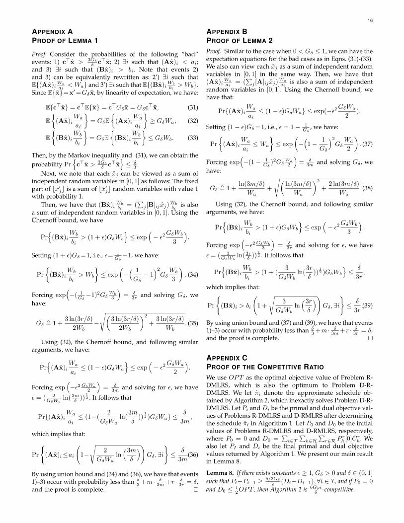
16

APPENDIX APROOF OF LEMMA 1

Proof. Consider the probabilities of the following “bad”events: 1) c>x > 3Gδ

δ c>x; 2) ∃i such that (Ax)i < ai;and 3) ∃i such that (Bx)i > bi. Note that events 2)and 3) can be equivalently rewritten as: 2’) ∃i such thatE{(Ax)i

Wa

ai< Wa} and 3’) ∃i such that E{(Bx)i

Wb

bi> Wb}.

Since E{x}=x′=Gδx, by linearity of expectation, we have:

E{c>x} = c>E{x} = c>Gδx = Gδc>x, (31)

E{

(Ax)iWa

ai

}= GδE

{(Ax)i

Wa

ai

}≥ GδWa, (32)

E{

(Bx)iWb

bi

}= GδE

{(Bx)i

Wb

bi

}≤ GδWb. (33)

Then, by the Markov inequality and (31), we can obtain theprobability Pr

{c>x > 3Gδ

δ c>x}≤ δ

3 .Next, we note that each xj can be viewed as a sum of

independent random variables in [0, 1] as follows: The fixedpart of bx′jc is a sum of bx′jc random variables with value 1with probability 1.

Then, we have that (Bx)iWb

bi= (

∑j [B]ij xj)

Wb

biis also

a sum of independent random variables in [0, 1]. Using theChernoff bound, we have

Pr{

(Bx)iWb

bi> (1 + ε)GδWb

}≤ exp

(− ε2GδWb

3

).

Setting (1 + ε)Gδ=1, i.e., ε= 1Gδ−1, we have:

Pr

{(Bx)i

Wb

bi> Wb

}≤ exp

(−( 1

Gδ− 1)2

GδWb

3

). (34)

Forcing exp(−( 1

Gδ−1)2Gδ

Wb

3

)= δ

3r and solving Gδ , wehave:

Gδ , 1 +3 ln(3r/δ)

2Wb−

√(3 ln(3r/δ)

2Wb

)2

+3 ln(3r/δ)

Wb. (35)

Using (32), the Chernoff bound, and following similararguments, we have:

Pr{

(Ax)iWa

ai≤ (1− ε)GδWa

}≤ exp

(− ε2GδWa

2

).

Forcing exp(−ε2GδWa

2

)= δ

3m and solving for ε, we have

ε = ( 2GδWa

ln( 3mδ ))

12 . It follows that

Pr{(Ax)iWa

ai≤ (1−(

2

GδWaln(

3m

δ))

12 )GδWa} ≤

δ

3m,

which implies that:

Pr

{(Ax)i≤ai

(1−

√2

GδWaln(3m

δ

))Gδ,∃i

}≤ δ

3m.(36)

By using union bound and (34) and (36), we have that events1)–3) occur with probability less than δ

3 +m · δ3m +r · δ3r = δ,and the proof is complete.

APPENDIX BPROOF OF LEMMA 2Proof. Similar to the case when 0 < Gδ ≤ 1, we can have theexpectation equations for the bad cases as in Eqns. (31)-(33).We also can view each xj as a sum of independent randomvariables in [0, 1] in the same way. Then, we have that(Ax)i

Wa

ai= (

∑j [A]ij xj)

Wa

aiis also a sum of independent

random variables in [0, 1]. Using the Chernoff bound, wehave that:

Pr{(Ax)iWa

ai≤ (1− ε)GδWa} ≤ exp(−ε2GδWa

2).

Setting (1− ε)Gδ=1, i.e., ε = 1− 1Gδ

, we have:

Pr

{(Ax)i

Wa

ai≤Wa

}≤ exp

(−(

1− 1

Gδ

)2

GδWa

2

). (37)

Forcing exp(−(1− 1

Gδ)2Gδ

Wa

2

)= δ

3m and solving Gδ , wehave:

Gδ , 1 +ln(3m/δ)

Wa+

√(ln(3m/δ)

Wa

)2

+2 ln(3m/δ)

Wa.(38)

Using (32), the Chernoff bound, and following similararguments, we have:

Pr{

(Bx)iWb

bi> (1 + ε)GδWb

}≤ exp

(− ε2GδWb

3

).

Forcing exp(−ε2GδWb

3

)= δ

3r and solving for ε, we have

ε = ( 3GδWb

ln( 3rδ ))

12 . It follows that

Pr{

(Bx)iWb

bi> (1 + (

3

GδWbln(

3r

δ))

12 )GδWb

}≤ δ

3r,

which implies that:

Pr

{(Bx)i > bi

(1 +

√3

GδWbln(3r

δ

))Gδ,∃i

}≤ δ

3r.(39)

By using union bound and (37) and (39), we have that events1)–3) occur with probability less than δ

3 +m · δ3m +r · δ3r = δ,and the proof is complete.

APPENDIX CPROOF OF THE COMPETITIVE RATIO

We use OPT as the optimal objective value of Problem R-DMLRS, which is also the optimum to Problem D-R-DMLRS. We let πi denote the approximate schedule ob-tained by Algorithm 2, which inexactly solves Problem D-R-DMLRS. Let Pi and Di be the primal and dual objective val-ues of Problems R-DMLRS and D-RMLRS after determiningthe schedule πi in Algorithm 1. Let P0 and D0 be the initialvalues of Problems R-DMLRS and D-RMLRS, respectively,where P0 = 0 and D0 =

∑t∈T

∑h∈H

∑r∈R P

rh [0]Crh. We

also let PI and Di be the final primal and dual objectivevalues returned by Algorithm 1. We present our main resultin Lemma 8.

Lemma 8. If there exists constants ε ≥ 1, Gδ > 0 and δ ∈ (0, 1]

such that Pi−Pi−1 ≥ δ/3Gδε (Di−Di−1),∀i ∈ I , and if P0 = 0

and D0 ≤ 12OPT , then Algorithm 1 is 6Gδε

δ -competitive.

17

Proof of Lemma 8. Since PI =∑i∈I

(Pi−Pi−1), and DI−D0 =∑i∈I

(Di −Di−1), we can have:

PI =∑i∈I

(Pi − Pi−1) ≥ δ/3Gδε

∑i∈I

(Di −Di−1)

=δ/3Gδε

(DI −D0).

By weak duality theorem [45], we have

DI ≥ OPT ≥ PI .

Thus, it follows that:

DI −D0 ≥1

2OPT,

PI ≥δ/3Gδε

(DI −D0) ≥ δ/3Gδ2ε

OPT,

and the proof is complete.

Next, following similar arguments in [6], [32], we in-troduce the relationship between the cost and resourceconsumption before and after processing one job. Let pr,ih [t]be the unit cost of type-r resource on server h at time t afterhandling job i. Let ρr,ih [t] be the amount of type-r resourceallocated to jobs on server h at time t after processingthe job i. For ease of our subsequent analysis, we nowdefine the following allocation-cost relation that is impliedby Algorithm 1:

Definition 1. The allocation-cost relationship for Algorithm 1with ε > 1, Gδ > 0 and δ ∈ (0, 1] is

pr,i−1h [t](ρr,ih [t]− ρr,i−1

h [t]) ≥ δ/3GδCrh

ε(pr,ih [t]− pr,i−1

h [t]),

∀i ∈ I, h ∈ H, r ∈ R.

The allocation-cost relationship shows that the cost ineach time slot for scheduling a new job is bounded by theincrease of term Crhp

rh[t] in Problem D-R-DMLRS, and the

possible increment introduced by randomized rounding inAlgorithm 4. This is ensured by the update of the pricefunction and the rounding scheme, respectively.

Lemma 9. If the allocation-cost relationship holds for ε ≥1, Gδ > 0 and δ ∈ (0, 1], then Algorithm 1 ensures Pi−Pi−1 ≥δ/3Gδε (Di −Di−1),∀i ∈ I .

Proof of Lemma 9. For any job i ∈ I , if job i is rejected,then we have Pi − Pi−1 = Di − Di−1 = 0 according toProblems R-DMLRS and D-R-DMLRS, the inequality musthold. If job i is accepted with schedule πi, i.e., xπi = 1, thenthe increment value of the primal objective value Pi is

Pi − Pi−1 = ui(tπi − ai).

Since xπi = 1, according to Algorithm 1, the constraint (11)is binding. Then, we can have

ui(tπi − ai)= λi +

∑t∈T (πi)

∑h∈H(πi[t])

∑r∈R

(αriwπiht + βri s

πiht)p

rh[t]

= λi +∑

t∈T (πi)

∑h∈H(πi[t])

∑r∈R

prh[t](ρr,ih [t]− ρr,i−1h [t]).

Similarly, we can have the increment value of the dualobjective value Di as follows:

Di −Di−1 =λi +∑

t∈T (πi)

∑h∈H(πi[t])

∑r∈R

(pr,ih [t]− pr,i−1h [t])Crh.

Summing up the allocation-cost relationship over all t ∈T (πi), h ∈ H(πi[t]), r ∈ R, we have

Pi − Pi−1 ≥δ/3Gδε

(Di −Di−1 − λi) + λi

=δ/3Gδε

(Di −Di−1) + (1− δ/3Gδε

)λi.

As λi ≥ 0, ε,Gδ > 0 and δ ∈ (0, 1], we have

Pi − Pi−1 ≥δ/3Gδε

(Di −Di−1).

This completes the proof of Lemma 9.

For specific h ∈ H, r ∈ R, we define εrh as the corre-sponding parameter in the allocation-cost relationship forany job i ∈ I and any time slot t ∈ T . Then, it holds thatε = maxh,r{εrh}. Without loss of generality, we assume thatthe resource demand of each worker or parameter serveris much smaller compared to the capacity of that resourceon one server, i.e., αri � Crh, β

ri � Crh. This is common in

real-world machine learning system as large percentage ofresources in the whole server. As ρrh[t] increases from 0 toCrh, then we can claim that dρrh[t] = ρr,ih − ρ

r,i−1h , and de-

rive a differential version of the allocation-cost relationship,which is defined as follows:

Definition 2. The differential allocation-cost relationship forAlgorithm 1 with εrh ≥ 1 is

prh[t]dρrh[t] ≥ Crhεrhdprh[t],∀t ∈ T , h ∈ H, r ∈ R.

Next we show that a feasible εrh satisfies the differentialallocation-cost relationship with price function prh[t] definedin (12).

Lemma 10. εrh = ln Ur

L , and the price function defined in (12)satisfy the differential allocation-cost relationship.

Proof of Lemma 10. The derivation of the marginal cost func-tion is

dprh[t] = pr′

h (ρrh[t])dρrh[t] = L(Ur

L)ρrh[t]

Crh ln(

Ur

L)

1Crh dρrh[t].

The differential allocation-cost relationship is

L(Ur

L)ρrh[t]

Crh dρrh[t] ≥ Crh

εrhL(Ur

L)ρrh[t]

Crh ln(

Ur

L)

1Crh dρrh[t],

which holds for εrh ≥ ln(Ur

L ). Then, we can set ε =

maxr∈R

(1, ln(Ur

L )), which satisfies the differential allocation-

cost relationship. This completes the proof.

With the aforementioned lemmas, we are now in aposition to prove Theorems 5 and 6. Note that the Theo-rems provide probabilistic guarantees. We first analyze theperformance ratio, which is followed by the probabilisticfeasibility discussion for both cases.

Proof of Theorems 5 and 6. According to Lemma 10, themarginal cost function used in Algorithm 1 satisfies

18

the differential allocation-cost relationship with ε =maxr(1, ln

Ur

L ). Since the resource demand in a job i is muchsmaller than the capacity, we can derive

dρrh[t] = ρr,ih − ρi−1h [t],

dprh[t] = pr′

h (ρrh[t])(ρr,ih [t]− ρr,i−1h [t]) = pr,ih [t]− pr,i−1

h [t].

So, the differential allocation-cost relationship in Defini-tion 2 implies the allocation-cost relationship in Definition 1holds for ε = maxr(1, ln

Ur

L ).According to Algorithm 1, we note that

1

µ≤dEiKi(τi + 2giγi/(b

(e)i Fi))e

∑r∈R(αri + βri )

T∑h∈H

∑r∈R C

rh

,∀i ∈ I.

Then, the minimum amount of overall resource consump-tion of job i can be computed as:

T∑h∈H

∑r∈R C

rh

µ

≤ dEiKi(τi + 2giγi/(b(e)i Fi))e

∑r∈R

(αri + βri ).

Then, it follows that:

D0 =∑t,h,r

LCrh

=∑t,h,r

mini∈I,πi∈Πi

1/(2µ)ui(tπi − ai)Crh∑r∈RdEiKi(τi + 2giγi/(b

(e)i Fi)e(αri + βri )

=T∑h,r C

rh

2µmini,πi

ui(tπi − ai)∑r∈RdEiKi(τi + 2giγi/(b

(e)i Fi)e(αri + βri )

≤ 1

2dEiKi(τi + 2giγi/(b

(e)i Fi))e

∑r∈R

(αri + βri )

mini∈I,πi∈Πi

ui(tπi − ai)∑r∈RdEiKi(τi + 2giγi/(b

(e)i Fi)e(αri + βri )

,∀i ∈ I.

(a)

≤ 1

2dEiKi(τi + 2giγi/(b

(e)i Fi))e

∑r∈R

(αri + βri )

ui(tπi − ai)∑r∈RdEiKi(τi + 2giγi/(b

(e)i Fi)e(αri + βri )

≤ 1

2ui(tπi − ai)

(b)

≤ 1

2OPT,

where (a) follows by selecting (i, π) =arg mini∈I,πi∈Πi ui(tπi − ai), and (b) follows from theassumption that the offline optimal solution accepts atleast one job, which is reasonable in real-world machinelearning system. Then we have OPT ≥ mini,π ui(tπi − ai).According to Lemmas 8 and 9, the competitive ratio isproved.

Recall that the randomized rounding algorithm is a keycomponent in our algorithm. Toward this end, we showthe probability of obtaining a feasible solution with theproved competitive ratio. Here, we consider the followingtwo cases:

1) When 0 < Gδ ≤ 1 (Theorem 5): According to The-orem 3, the probability of violating the cover constraint isno greater than δ/3 at each randomized rounding iteration.Recall that our Algorithm 1 runs a predetermined numberof S iterations to find a feasible integer solution. Thus the

probability that no feasible integer solution returned afterS iterations rounding is at most (δ/3)S . It then follows thatthe probability of at least one feasible integer solution foundis at least 1 − (δ/3)S . Moreover, the number of states (t, v)in the dynamic programming for each job i is O(TKiEi).Therefore, with probability greater than (1− (δ/3)S)TiKiEi ,PD-ORS in Algorithm 1 returns a feasible integer solutionwith the proved competitive ratio.

2) When Gδ > 1 (Theorem 6): According to Theorem 4,the probability of violating the packing constraint is nogreater that δ/3(HR + 1) at each randomized roundingiteration. Following the similar arguments in 1), we canshow that with probability greater than (1 − (δ/3(HR +1))S)TiKiEi , PD-ORS in Algorithm 1 returns a feasible in-teger solution with the proved competitive ratio, and theproof is complete.