Embed Size (px)
Citation preview

Didacticiel - Études de cas R.R.
4 novembre 2012 Page 1
1 Topic
Linear Discriminant Analysis – Data Mining Tools Comparison (Tanagra, R, SAS and SPSS).
Linear discriminant analysis is a popular method in domains of statistics, machine learning and
pattern recognition. Indeed, it has interesting properties: it is rather fast on large bases; it can handle
naturally multi-class problems (target attribute with more than 2 values); it generates a linear
classifier linear, easy to interpret; it is robust and fairly stable, even applied on small databases; it has
an embedded variable selection mechanism. Personally, I appreciate linear discriminant analysis
because we can have multiple interpretations (probabilistic, geometric), and thus highlights various
aspects of supervised learning.
Discriminant analysis is both a descriptive and a predictive method1. In the first case, we say
Canonical Discriminant Analysis. We can consider the approach as a dimension reduction technique
(a factor analysis). We want to highlight latent variables which explain the difference between the
classes defined by the target attribute. In the second case, we can consider the approach as a
supervised learning algorithm which intends to predict efficiently the class membership of
individuals. Because we have a linear combination of the variables, we have a linear classifier. The
purposes are therefore not intrinsically identical even if, when we analyze deeply the underlying
formulas, we realize that the two approaches are closely related. Some bibliographic references
maintain anyway the confusion by presenting them in a single framework.
Tanagra differentiates clearly the two approaches by providing two separate components: LINEAR
DISCRIMINANT ANALYSIS (SPV LEARNING tab) for the prediction approach; CANONICAL
DISCRIMINANT ANALYSIS (FACTORIAL ANALYSIS tab) for the descriptive (factorial) approach. It is the
same for SAS software with respectively DISCRIM and CANDISC procedures2. Others combine them.
This is the case for SPSS and R, mixing results which refer to different goals. For specialists who know
how to distinguish important elements depending on the context, this amalgam is not a problem. For
beginners, it is a bit more problematic. One can be disturbed by results which do not seem directly
related to the purposes of the study.
In this tutorial, we detail in a first time with the TANAGRA outputs about Predictive Linear
Discriminant Analysis. In a second time, we compare them to the results of R, SAS and SPSS. The
objective is to identify important information for predictive analysis i.e. get a simple classification
system, get indications on the influence (for the interpretation) and the relevance of variables
(statistical significance), and dispose of a variable selection mechanism.
2 Dataset We use the « alcohol.xls » data file. We want to predict the alcohol type (Kirsch, Mirabelle and Pear)
from their composition (butanol, etc.; 6 descriptors). The sample contains 77 instances.
1 http://en.wikipedia.org/wiki/Linear_discriminant_analysis, http://en.wikipedia.org/wiki/Discriminant_function_analysis
The distinction between the two approaches is clearly defined on the French version of Wikipedia
(http://fr.wikipedia.org/wiki/Analyse_discriminante - http://fr.wikipedia.org/wiki/Analyse_discriminante_linéaire).
2 http://support.sas.com/documentation/

Didacticiel - Études de cas R.R.
4 novembre 2012 Page 2
3 Linear discriminant analysis under Tanagra
3.1 Importing dataset
After we launch Tanagra, we create a new diagram by clicking on the FILE / NEW menu. We select
the “alcohol.xls” data file.
Tanagra shows the number of instances (77) and the number of variables (7, including the class
attribute TYPE) which are loaded.

Didacticiel - Études de cas R.R.
4 novembre 2012 Page 3
3.2 Linear discriminant analysis
The DEFINE STATUS enables to specify the status of the variables in the analysis: TYPE is the target
attribute (TARGET); the others are the descriptors (INPUT).
We add the LINEAR DISCRIMINANT ANALYSIS (SPV LEARNING tab) into the diagram. We click on the
contextual menu VIEW to obtain the results.
Didacticiel - Études de cas R.R.
4 novembre 2012 Page 4
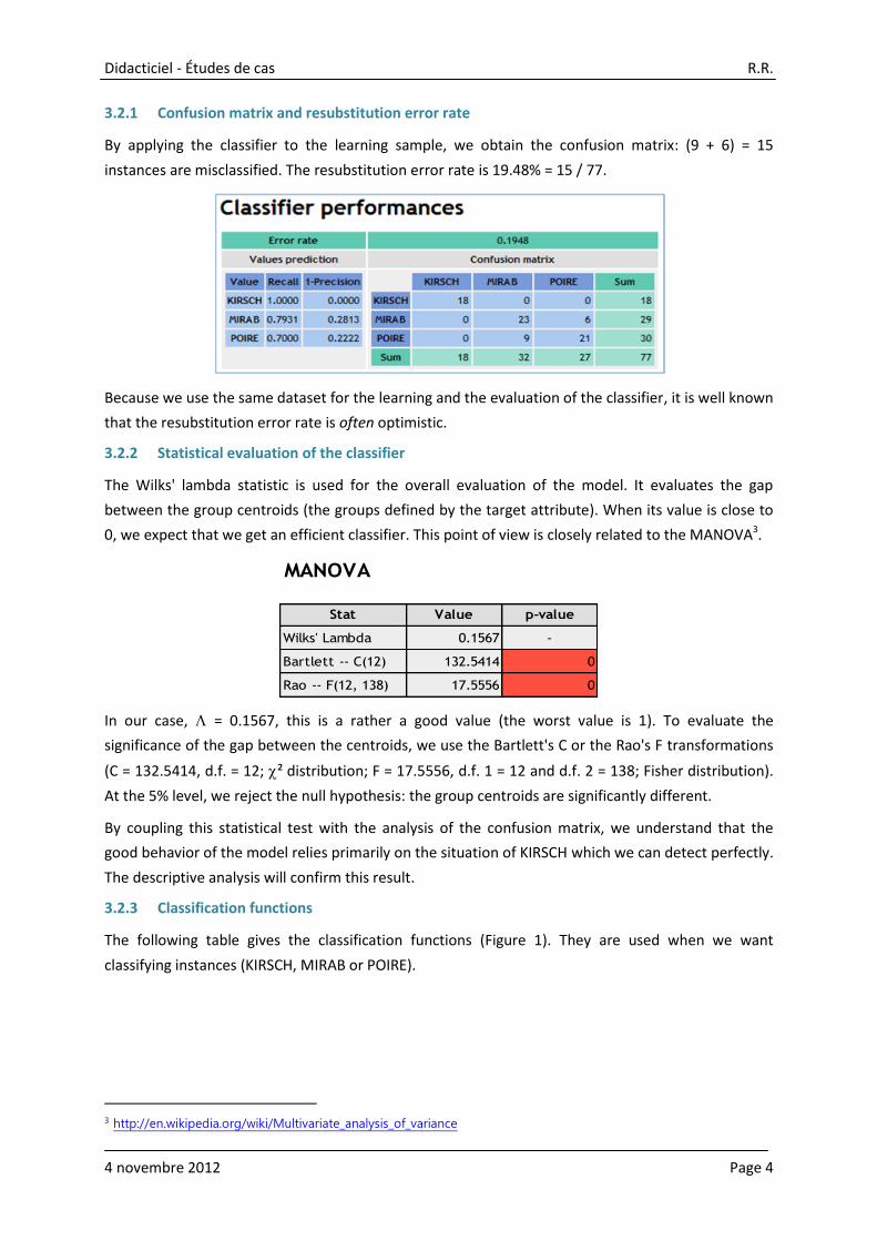
3.2.1 Confusion matrix and resubstitution error rate
By applying the classifier to the learning sample, we obtain the confusion matrix: (9 + 6) = 15
instances are misclassified. The resubstitution error rate is 19.48% = 15 / 77.
Because we use the same dataset for the learning and the evaluation of the classifier, it is well known
that the resubstitution error rate is often optimistic.
3.2.2 Statistical evaluation of the classifier
The Wilks' lambda statistic is used for the overall evaluation of the model. It evaluates the gap
between the group centroids (the groups defined by the target attribute). When its value is close to
0, we expect that we get an efficient classifier. This point of view is closely related to the MANOVA3.
MANOVA
Stat Value p-value
Wilks' Lambda 0.1567 -
Bartlett -- C(12) 132.5414 0
Rao -- F(12, 138) 17.5556 0
In our case, = 0.1567, this is a rather a good value (the worst value is 1). To evaluate the
significance of the gap between the centroids, we use the Bartlett's C or the Rao's F transformations
(C = 132.5414, d.f. = 12; ² distribution; F = 17.5556, d.f. 1 = 12 and d.f. 2 = 138; Fisher distribution).
At the 5% level, we reject the null hypothesis: the group centroids are significantly different.
By coupling this statistical test with the analysis of the confusion matrix, we understand that the
good behavior of the model relies primarily on the situation of KIRSCH which we can detect perfectly.
The descriptive analysis will confirm this result.
3.2.3 Classification functions
The following table gives the classification functions (Figure 1). They are used when we want
classifying instances (KIRSCH, MIRAB or POIRE).
3 http://en.wikipedia.org/wiki/Multivariate_analysis_of_variance

Didacticiel - Études de cas R.R.
4 novembre 2012 Page 5
Attribute KIRSCH MIRAB POIRE
MEOH 0.000659 0.015208 0.016407
ACET 0.000445 0.004944 -0.00377
BU1 -0.039342 0.556654 0.553048
MEPR 0.186892 0.035901 0.102271
ACAL 0.039174 -0.160881 -0.127328
LNPRO1 6.378935 4.86937 5.34143
constant -24.686164 -25.141755 -29.631644
Classification functions
Figure 1 – Classification functions - Model without variable selection
Let us consider a new unlabeled instance to classify.
MEOH ACET BU1 MEPR ACAL LNPRO1
707.0 131.0 15.0 28.0 9.0 4.89
We apply the classification function for each class value. For instance, for KIRSCH we have:
S(, KIRSCH) = 0.000659 x 707 + 0.000445 x 131 – 0.039342 x 15 + 0.186892 x 28 + 0.039174 x 9 +
6.378935 x 4.89 – 24.68616 = 12.0264
We apply the function for each class, we obtain:
KIRSCH MIRAB POIRE
S(.) 12.0264 17.9763 17.6072
MIRAB has the highest score [S(MIRAB) = 17.9763]. We assign the value MIRAB to this instance.
This classification operation is one of the main goals of the predictive analytics process.
3.2.4 Assessing the influence of the variables in the model
The influence of the predictive variables is not the same. The discriminant analysis can measure their
contribution in the model. Tanagra shows these effects in the Statistical Evaluation part of the
coefficients table (green).
Attribute KIRSCH MIRAB POIRE Wilks L. Partial L. F(2,69) p-value
MEOH 0.000659 0.015208 0.016407 0.205214 0.763359 10.69497 0.00009
ACET 0.000445 0.004944 -0.00377 0.176705 0.88652 4.41622 0.015677
BU1 -0.039342 0.556654 0.553048 0.213115 0.73506 12.43496 0.000024
MEPR 0.186892 0.035901 0.102271 0.192667 0.813074 7.93155 0.000793
ACAL 0.039174 -0.160881 -0.127328 0.161541 0.969735 1.07671 0.346369
LNPRO1 6.378935 4.86937 5.34143 0.171693 0.912399 3.31241 0.042303
constant -24.686164 -25.141755 -29.631644
Classification functions Statistical Evaluation
-
Remember that the overall lambda of the model is = 0.1567 (Section 3.2.2).
The first column (“Wilks L.”) indicates the lambda of the model if we remove the variable. For
instance, if we remove MEOH from the classifier, the new value of the lambda for the model
containing all the predictive variables except MEOH is {-MEOH} = 0.205214. The higher is the
difference with the initial value of lambda, the most significant is the variable. “Partial lambda” is the
ratio between these values. For instance, Partial L.{-MEOH} = 0.1567 / 0.205214 = 0.763.

Didacticiel - Études de cas R.R.
4 novembre 2012 Page 6
The last two columns are dedicated to the checking of the contribution of each variable. They are
based on the comparison of the lambda with and without the variable that we intend to evaluate.
For our dataset, only ACAL is not significant at the 5% level (p-value{-ACAL} = 0.346369 > 5%).
3.3 Variable selection
We can select the relevant variables by using a stepwise approach.
For this, we use the STEPDISC (FEATURE SELECTION tab) component. Tanagra can implement forward
and backward strategies. We choose the forward strategy for our dataset. We start with the null
model. We add sequentially the most significant variable as long as it is significant at the 1% level.

Didacticiel - Études de cas R.R.
4 novembre 2012 Page 7
Because we add STEPDISC after DEFINE STATUS 1 into the diagram, it searches the relevant variables
among those defined as INPUT into the preceding component. We click on the VIEW menu to obtain
the results, 3 variables are selected: BU1, MEPR, MEOH
Tanagra provides the details of the search processing. We will describe them later (cf. SAS outputs).
All we need to do is to add again the LINEAR DISCRIMINANT ANALYSIS component after STEPDISC
into the diagram. Tanagra performs the learning process on the selected variables only.
The resubstitution error rate is 25.97%. It seems worse than the model with all the predictive
attributes (19.48%). But we know that the resubstitution error rate is not a good indicator of the
performance of the models. It often favors the complex model incorporating a large number of
predictive variables. We must use resampling approach (e.g. cross validation, bootstrap) to obtain a
reliable evaluation of the error rate enabling to compare the models.
Here are the coefficients of the new classification functions.
Figure 2 – Classification functions – Model after variable selection
We apply the new model on the instance to classify (section 3.2.3, the unused variables are grayed):
MEOH ACET BU1 MEPR ACAL LNPRO1
707.0 131.0 15.0 28.0 9.0 4.89
We obtain the following scores. Here also, we assign the instance to the MIRAB class.
KIRSCH MIRAB POIRE
S(.) 1.4610 6.2670 5.5103
Attribute KIRSCH MIRAB POIRE Wilks L. Partial L. F(2,72) p-value
BU1 -0.19402 0.432081 0.43508 0.303303 0.66354 18.25443 0
MEPR 0.158883 0.016375 0.080243 0.251168 0.801272 8.92855 0.000344
MEOH 0.007296 0.018626 0.019405 0.248931 0.808472 8.52844 0.000474
constant -5.235679 -13.841347 -16.982045
Classification functions Statistical Evaluation
-

Didacticiel - Études de cas R.R.
4 novembre 2012 Page 8
3.4 Canonical discriminant analysis (factorial discriminant analysis)
Descriptive discriminant analysis is not the main topic of this tutorial. But we present nevertheless
the outputs of Tanagra to better understand the results provided of the other tools.
We add the CANONICAL DISCRIMINANT ANALYSIS (FACTORIAL ANALYSIS tab) component into the
diagram. Then we click on the VIEW menu to obtain the results.
3.4.1 Eigenvalues table
This table provides the eigenvalues for each factor. We have also the proportion of explained
variance. The significance test of each factor is provided.
Roots and Wilks' Lambda
Root Eigenvalue Proportion Canonical R Wilks Lambda CHI-2 d.f. p-value
1 3.75959 0.9168 0.888762 0.156652 132.5414 12 0
2 0.3412 1 0.504381 0.7456 20.99 5 0.000814
3.4.2 Canonical coefficients
The raw canonical coefficients enable to calculate the coordinate of the individuals on the factors.
The unstandardized coefficients can be applied on the untransformed values of the variables.
Canonical Discriminant Function
Coefficients
Attribute Root n1 Root n2 Root n1 Root n2
MEOH -0.0033821 -0.000571 -0.6811478 -0.1150081
ACET 0.0000465 0.0066574 0.0051822 0.7420478
BU1 -0.1322048 0.0162599 -0.6469978 0.0795743
MEPR 0.0256226 -0.053361 0.3454686 -0.7194653
ACAL 0.0404876 -0.0297884 0.2160076 -0.1589256
LNPRO1 0.2791911 -0.3894401 0.2753705 -0.3841107
constant 1.89673943 3.17877051
Unstandardized Standardized
-
Figure 3 – Raw canonical coefficients
For the instance with the following description:

Didacticiel - Études de cas R.R.
4 novembre 2012 Page 9
MEOH ACET BU1 MEPR ACAL LNPRO1
707.0 131.0 15.0 28.0 9.0 4.89
The coordinate on the first factor is,
Axe 1 = -0.0033821 x 707 + 0.0000465 x 131 – 0.1322048 x 15 + 0.0256226 x 28 + 0.0404876 x 9 +
0.2791911 x 4.89 + 1.89673943 = -0.0243
On the second factor, Axe 2 = -0.000571 x 707 + … - 0.3894401 x 4.89 + 3.17877051 = 0.2245
By applying these functions on the individuals of the learning sample, we obtain a representation of
the instances into the two first axes. By coloring the points according to its group membership, we
can evaluate the class separability. We note that KIRSCH does not overlap of the others. This
confirms the results of the confusion matrix obtained earlier (section 3.2.1).
3.4.3 Canonical structure
The canonical structure corresponds to the correlation between the variables and the factors. There
are different ways to compute this correlation: ignoring the class membership (TOTAL); controlling
the class membership (WITHIN); highlighting the class membership (BETWEEN).
Factor Structure Matrix - Correlations
Root
Descriptors Total Within Between Total Within Between
MEOH -0.890038 -0.676771 -0.991413 -0.206864 -0.296316 -0.130768
ACET 0.044423 0.021247 0.138243 0.560792 0.505278 0.990398
BU1 -0.939650 -0.787683 -0.997447 -0.118534 -0.187184 -0.071407
MEPR -0.171747 -0.086008 -0.378992 -0.738951 -0.697111 -0.925400
ACAL -0.159216 -0.073841 -0.929377 -0.111430 -0.097353 -0.369131
LNPRO1 0.521401 0.272151 0.968743 -0.235265 -0.231331 -0.248066
Root n1 Root n2
At a first glance, we observe that: (1) the distinction between KIRSCH and the others relies mainly on
MEOH and BU1 on the first axis; (2) the distinction between MIRAB and POIRE on the second axis is
due to ACET and MEPR.
-4
-3
-2
-1
0
1
2
3
4
-5 -3 -1 1 3 5
Can
on
ical
co
mp
on
en
t 2
Canonical component 1
Canonical components scatter plot
KIRSCH
MIRAB
POIRE
Didacticiel - Études de cas R.R.
4 novembre 2012 Page 10
These results are consistent with the predictive approach where BU1, MEPR and MEOH were the
selected variables after the STEPDISC FORWARD process at 1% level.
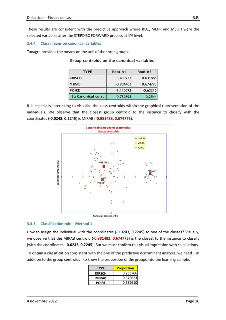
3.4.4 Class means on canonical variables
Tanagra provides the means on the axis of the three groups.
Group centroids on the canonical variables
TYPE Root n1 Root n2
KIRSCH 3.439733 -0.031885
MIRAB -0.981483 0.674773
POIRE -1.115073 -0.63315
Sq Canonical corr. 0.789898 0.2544
It is especially interesting to visualize the class centroids within the graphical representation of the
individuals. We observe that the closest group centroid to the instance to classify with the
coordinates (-0.0243, 0.2245) is MIRAB (-0.981483, 0.674773).
3.4.5 Classification rule – Method 1
How to assign the individual with the coordinates (-0.0243, 0.2245) to one of the classes? Visually,
we observe that the MIRAB centroid (-0.981483, 0.674773) is the closest to the instance to classify
(with the coordinates: -0.0243, 0.2245). But we must confirm this visual impression with calculations.
To obtain a classification consistent with the one of the predictive discriminant analysis, we need – in
addition to the group centroids - to know the proportion of the groups into the learning sample.
TYPE Proportion
KIRSCH 0.233766
MIRAB 0.376623
POIRE 0.389610
-4
-3
-2
-1
0
1
2
3
4
-5 -4 -3 -2 -1 0 1 2 3 4 5
Can
on
ical
co
mp
on
en
t 2
Canonical component 1
Canonical components scatter plot
Group centroids
KIRSCH
MIRAB
POIRE
KIRSCH
MIRAB
POIRE

Didacticiel - Études de cas R.R.
4 novembre 2012 Page 11
For the instance that we want to classify, we calculate the squared generalized distance to the
centroids:
Where c is one the classes, K is the number of factors, fk() is the coordinate of the instance on the
factor k, kc is the conditional mean of the class c on the factor k, πc is the proportion of the class c in
the learning sample.
Thus, for the various classes, we obtain:
D²(, KIRSCH) = (-0.0243 – 3.439733)² + (0.2245 + 0.031885)² - 2 ln(0.233766) = 14.9723
D²(, MIRAB) = (-0.0243 + 0.981483)² + (0.2245 – 0.376623)² - 2 ln(0.376623) = 3.0719
D²(, POIRE) = (-0.0243 + 1.115073)² + (0.2245 + 0.63315)² - 2 ln(0.389610) = 3.8106
We assign the individual to the class for which the centroid is the closest. In this case, this is MIRAB
since D²(, MIRAB) takes the smallest value.
Furthermore, we can calculate the posterior probability of the class membership:
For the instance above:
P(Y() = KIRSCH / X) = 0.00056 / 0.36459 = 0.00154
P(Y() = MIRAB / X) = 0.21525 / 0.36459 = 0.59039
P(Y() = POIRE / X) = 0.14878 / 0.36459 = 0.40807
We assign the instance to the most likely group.
3.4.6 Classification rule - Method 2
By developing the formulas above and by multiplying them by -0.5, we obtain a linear classification
functions based on the factorial coordinates. They are equivalent to the classification function
provided by the predictive discriminant analysis, to within a constant which does not depend to the
class membership. So, the classification characteristic is exactly the same.
We have:
For the instance to classify:
S’(, KIRSCH) = -0.0243 x 3.439733 + 0.2245 x (-0.031885) – (3.439733² + (-0.031885)²)/2 + ln(0.233766) = -7.4606
S’(, MIRAB) = -0.0243 x (-0.981483) + 0.2245 x 0.674773 – ((-0.981483)² + 0.674773²)/2 + ln(0.376623) = -1.5105
S’(, POIRE) = -0.0243 x (-1.115073) + 0.2245 x (-0.63315) – ((-1.115073)² + (-0.63315) ²)/2 + ln(0.389610) = -1.8798
We assign the instance to the MIRAB class. The result is necessarily consistent with that of the
predictive discriminant analysis (sections 3.2.3 and 3.4.5).

Didacticiel - Études de cas R.R.
4 novembre 2012 Page 12
3.4.7 Classification rule - Return on the original variables - Method 3
In the previous section, the classification functions are a linear combination of the factors. These last
ones are a linear combination of the original variables. So, we can produce a classification function
defined on the original predictive variables.
The classification functions on factors are the following:
Score function 1 KIRSCH MIRAB POIREf1 3.439733 -0.981483 -1.115073f2 -0.031885 0.674773 -0.633150Const -7.369825 -1.685824 -1.764742
For instance, we have for KIRSH: S’(KIRSH) = 3.439733 x f1 -0.031885 x f2 – 7.369825
The factors F1 are F2 are linear combinations of original predictive attributes (Figure 3). We can thus
produce a new version of the classification functions defined on the predictive attributes S’(.):
Score function 2 KIRSCH MIRAB POIREMEOH -0.011615 0.002934 0.004133ACET -0.000052 0.004447 -0.004267BU1 -0.455268 0.140729 0.137123MEPR 0.089836 -0.061155 0.005214ACAL 0.140216 -0.059838 -0.026286LNPRO1 0.972760 -0.536805 -0.064744constant -0.946902 -1.402493 -5.892384
We can compare them to the classification functions obtained from the predictive linear discriminant
analysis S(.) (Figure 1). We observe that the coefficients of S() and S'() are different, but the gap
between the classes is the same for each variable.
This is the reason for which we have not the same score value for the individual
S(, KIRSCH) ≠ S’(, KIRSCH) ; S(, MIRAB) ≠ S’(, MIRAB) ; S(, POIRE) ≠ S’(, POIRE)
But the difference depends on the individual and not to the class membership.
[S(, KIRSCH) - S’(, KIRSCH)] = [S(, MIRAB) - S’(, MIRAB)] = [S(, POIRE) - S’(, POIRE)]
In the end, the instances are classified in identical way. This is the most important.
4 Discriminant analysis under SAS
4.1 Proc DISCRIM
We perform the same analysis under SAS 9.3 using PROC DISCRIM. We use the following commands.
Attribute KIRSCH MIRAB POIRE KIRSCH MIRAB POIRE KIRSCH MIRAB POIRE
MEOH 0.000659 0.015208 0.016407 -0.011615 0.002934 0.004133 0.0123 0.0123 0.0123
ACET 0.000445 0.004944 -0.003770 -0.000052 0.004447 -0.004267 0.0005 0.0005 0.0005
BU1 -0.039342 0.556654 0.553048 -0.455268 0.140729 0.137123 0.4159 0.4159 0.4159
MEPR 0.186892 0.035901 0.102271 0.089836 -0.061155 0.005214 0.0971 0.0971 0.0971
ACAL 0.039174 -0.160881 -0.127328 0.140216 -0.059838 -0.026286 -0.1010 -0.1010 -0.1010
LNPRO1 6.378935 4.869370 5.341430 0.972760 -0.536805 -0.064744 5.4062 5.4062 5.4062
constant -24.686164 -25.141755 -29.631644 -0.946902 -1.402493 -5.892384 -23.7393 -23.7393 -23.7393
Ecarts entre coefficientsS'() - Déduite de l'analyse descriptiveS() - Analyse prédictive

Didacticiel - Études de cas R.R.
4 novembre 2012 Page 13
proc discrim data = alcohol;
class type;
var MEOH ACET BU1 MEPR ACAL LNPRO1;
priors proportional;
run;
The PRIORS option enables to use the proportion measured on the learning set as classes’ prior
distribution in the learning process.
METHOD = NORMAL (multivariate normal distribution) and POOL = YES (used the pooled covariance
matrix) are two important options for which the default values were used.
Overall description. SAS provides a description of the problem that we handle. We observe, among
others, the proportion of classes into the learning sample.
Distances between the group centroids. We have the squared generalized distance between the
group centroids.
The distance between the centroids of the same group is not null. In addition it is not symmetric!

Didacticiel - Études de cas R.R.
4 novembre 2012 Page 14
This is really surprising. This is because the proportion of the groups is used in the formula4. For
instance, the distance of the KIRSCH with itself is obtained with (see section 3.4.4 for the values of
the centroids):
D²(KIRSCH, KIRSCH) = (3.439733 - 3.439733)² + (-0.031885 + 0.031885)² – 2 x ln(0.233766) = 2.90687
The generalized distance is not symmetric. For instance, between KIRSCH and MIRAB:
D²(KIRSCH, MIRAB) = (3.439733 + 0.981483)² + (-0.031885 – 0.674773)² - 2 x ln(0.233766) = 22.95339
D²(MIRAB, KIRSCH) = (-0.981483 – 3.439733)² + (0.674773 + 0.031885)² -2 x ln(0.376623) = 21.99954
Classification functions. SAS provides the same classification functions as Tanagra.
But SAS does not provide any information about the relevance of the variables.
Confusion matrix and resubstitution error rate. Last, SAS provides the confusion matrix.
4 http://www.math.wpi.edu/saspdf/stat/chap25.pdf

Didacticiel - Études de cas R.R.
4 novembre 2012 Page 15
4.2 Variable selection with STEPDISC
SAS proposes STEPDISC, a tool for the variable selection which is consistent with the linear
discriminant analysis principle. We perform a forward selection at 1% level (METHOD = FORWARD,
SLENTRY = 1%):
proc stepdisc data = alcohol method = forward slentry = 0.01;
class type;
var MEOH ACET BU1 MEPR ACAL LNPRO1;
run;
We compare the detailed results with those of Tanagra (Figure 4).
Figure 4 – Detailed results - Stepdisc at 1% level - Tanagra
Step 1: SAS picks BU1 after having listed the contributions of the candidate variables.
SAS
TANAGRA

Didacticiel - Études de cas R.R.
4 novembre 2012 Page 16
SAS provides R-Square = 1 - . For instance, R-Square(MEOH) = 1 – 0.363 = 0.6366. The F statistic is
the same as Tanagra, it enables to check the significance of the variable e.g. F(MEOH) = 64.82, with
the p-value(MEOH) = 0.0001. The tolerance statistic characterizes the redundancy with the variables
already included in the model. At the first step, the initial set of selected variables is empty. There is
no possible redundancy. It is therefore equal to 1 for all variables.
BU1 has the highest "F Value", and it is significant at the 1% level. It is thus included in the model. In
the forward process, this decision is unchangeable. We cannot remove this variable later.
SAS pursues with the assessment of the current model
The stepdisc documentation explains the reading of the various statistics (Pillai, Average Squared
Canonical Correlation) provided by SAS. There is one variable at this step. Thus, the “F Value” is the
same as the one of the BU1 variable in the table “Stepdisc Procedure – Step 1” above.
Step 2: SAS evaluates the contribution of the remaining variables. The "Partial R-Square" compares
the lambda of the models containing or not an additional variable e.g. for MEOH, Partial R-
Square(MEOH) = 1 – 0.251 / 0.299 0.160.
MEPR is the best variable according the “Partial R-Square” (or according to the F Value). It is
significant at the 1% level. It is approved.
We note also, even if this is not taken into account for the selection, that MEPR is weakly correlated
with the already introduced variable because its tolerance is 0.9046. It means that the squared
correlation between BU1 and MEPR is r² = 1 – 0.9046 = 0.0954.
For the overall evaluation of the model with 2 (BU1, MEPR) predictive variables, we have:
SAS
TANAGRA

Didacticiel - Études de cas R.R.
4 novembre 2012 Page 17
SAS continues until it is no more possible to add variables. It then produces a table summarizing the
process (Figure 5). The values (Wilks lambda, F Value) are consistent with those of Tanagra.
Figure 5 – Summary of the selection process - Stepdisc forward at 1% level
The selected variables are: BU1, MEPR and MEOH.
5 Discriminant Analysis under R – lda() [MASS package]
We use the lda() procedure of the « MASS » package to perform the linear discriminant analysis. This
package is automatically installed with R.
5.1 Importing the dataset
The read.xlsx() command of the package “xlsx”5 enables to read a data file in the Excel format (XLS or
XLSX). The summary() command describes shortly the variables of the dataset.
library(xlsx)
#sheetIndex: number of the sheet to read
#header: the first row corresponds to the name of the variables
alcohol.data <- read.xlsx(file="alcohol.xls",sheetIndex=1,header=T)
print(summary(alcohol.data))
We obtain the main features of the variables.
5 http://cran.r-project.org/web/packages/xlsx/index.html
SASTANAGRA

Didacticiel - Études de cas R.R.
4 novembre 2012 Page 18
TYPE is the categorical attribute (3 values) that we want to explain.
5.2 Using the lda() procedure
We load the MASS6 package. We start the lda() procedure on the learning sample.
#linear discriminant analysis
library(MASS)
alcohol.lda <- lda(TYPE ~ ., data = alcohol.data)
print(alcohol.lda)
lda() provides: the proportions of the classes; the conditional mean of the variables according to the
classes; the unstandardized coefficients of the canonical functions (Section 3.4.2), without the
constant term; the proportion of variance explained by each factor.
6 http://cran.r-project.org/web/packages/MASS/index.html

Didacticiel - Études de cas R.R.
4 novembre 2012 Page 19
In principle, lda() seems only intended to the descriptive analysis. But as we have seen above, the
connection between the descriptive analysis and the predictive analysis is strong (section 3.4.5).
Thus, the predict() command enables to assign individual to the classes. The classification properties
are identical to those of Tanagra or SAS i.e. each individual is assigned to the same group whatever
the tool used.
5.3 Prediction
The predict() enables to apply the classifier on the individuals.
#prediction on the training set
pred.lda <- predict(alcohol.lda,newdata=alcohol.data)
print(attributes(pred.lda))
The object has 3 main properties: ‘class’, ‘posterior’ and ‘x’.
‘class’ is a vector, its length is n = 77. It provides the predicted value for each individual of the
sample. For instance, we show here the predicted values for the first 6 individuals.
‘posterior’ is a matrix with n = 77 rows and 3 columns (because the class attribute has 3 values). Each
column corresponds to the posterior probability of the class membership. For the first 6 instances,
we have the following values:
‘x’ provides the canonical coordinates of the instances. This is a matrix with 77 rows and 2 columns
(because we have two factors). Here are the values for the first 6 instances:

Didacticiel - Études de cas R.R.
4 novembre 2012 Page 20
5.4 Confusion matrix
To obtain the confusion matrix, we create a contingency table from the observed values of the class
attribute and the predictions of the model.
#confusion matrix
mc.lda <- table(alcohol.data$TYPE,pred.lda$class)
print(mc.lda)
We have the same matrix as Tanagra (section 3.2.1) and SAS (section 4.1).
We can compute the error rate,
#error rate
print(1-sum(diag(mc.lda))/sum(mc.lda))
We have 19.48%
5.5 Variable selection
We use the proceduree greedy.wilks() of the package « klaR »7 for the variable selection.
#variable selection
library(klaR)
alcohol.forward <- greedy.wilks(TYPE ~ .,data=alcohol.data, niveau = 0.01)
7 http://cran.r-project.org/web/packages/klaR/index.html
Didacticiel - Études de cas R.R.
4 novembre 2012 Page 21
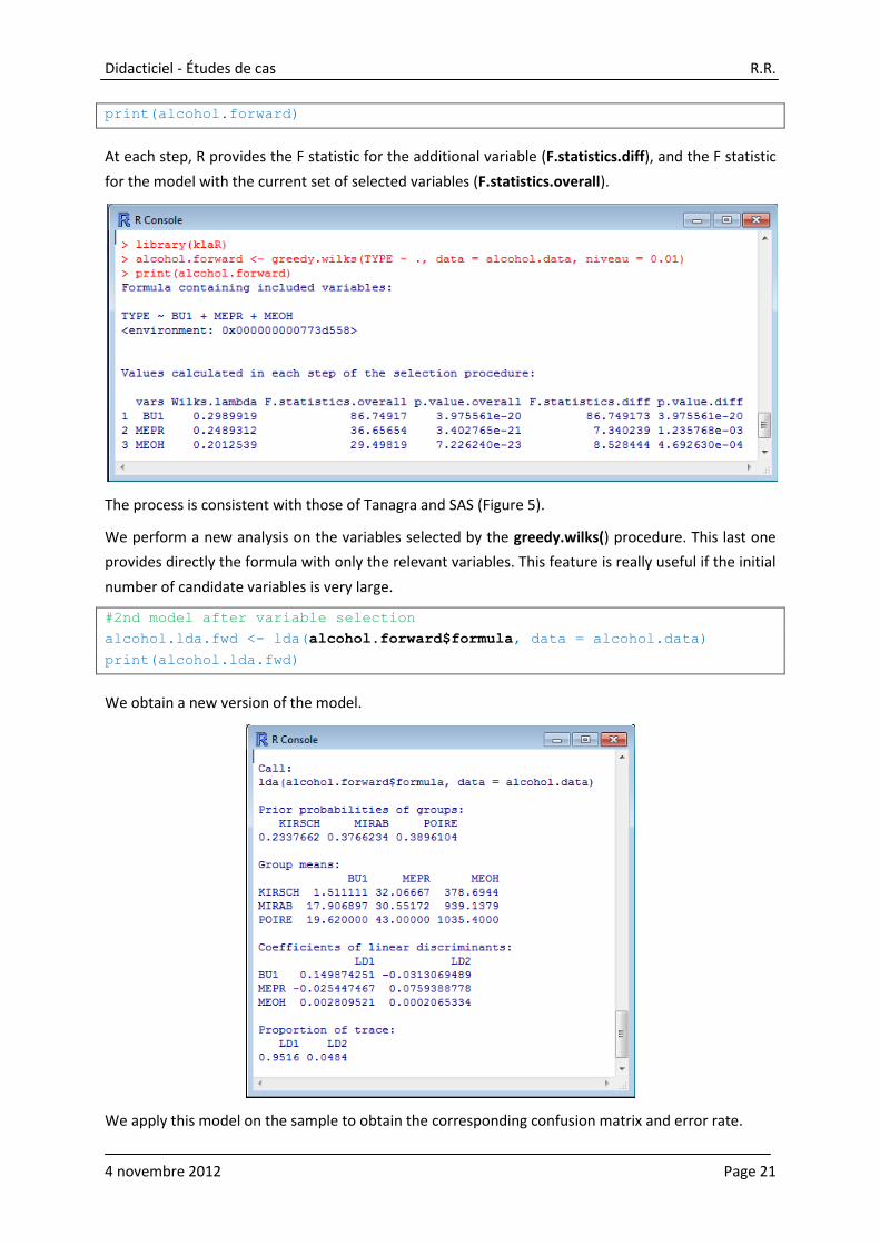
print(alcohol.forward)
At each step, R provides the F statistic for the additional variable (F.statistics.diff), and the F statistic
for the model with the current set of selected variables (F.statistics.overall).
The process is consistent with those of Tanagra and SAS (Figure 5).
We perform a new analysis on the variables selected by the greedy.wilks() procedure. This last one
provides directly the formula with only the relevant variables. This feature is really useful if the initial
number of candidate variables is very large.
#2nd model after variable selection
alcohol.lda.fwd <- lda(alcohol.forward$formula, data = alcohol.data)
print(alcohol.lda.fwd)
We obtain a new version of the model.
We apply this model on the sample to obtain the corresponding confusion matrix and error rate.
Didacticiel - Études de cas R.R.
4 novembre 2012 Page 22
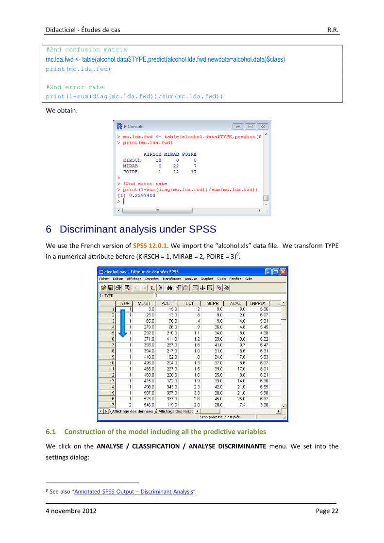
#2nd confusion matrix
mc.lda.fwd <- table(alcohol.data$TYPE,predict(alcohol.lda.fwd,newdata=alcohol.data)$class)
print(mc.lda.fwd)
#2nd error rate
print(1-sum(diag(mc.lda.fwd))/sum(mc.lda.fwd))
We obtain:
6 Discriminant analysis under SPSS
We use the French version of SPSS 12.0.1. We import the “alcohol.xls” data file. We transform TYPE
in a numerical attribute before (KIRSCH = 1, MIRAB = 2, POIRE = 3)8.
6.1 Construction of the model including all the predictive variables
We click on the ANALYSE / CLASSIFICATION / ANALYSE DISCRIMINANTE menu. We set into the
settings dialog:
8 See also “Annotated SPSS Output – Discriminant Analysis”.

Didacticiel - Études de cas R.R.
4 novembre 2012 Page 23
We set TYPE in « Critère de regroupement », the range (Définir intervalle) of the value is MIN = 1 to
MAX = 3. All the others variables are predictive variables « Variables explicatives ». At the moment,
we do not perform a variable selection « Entrer les variables simultanément ».
Then, we click on the « Statistiques » button. We ask the “Fisher” classification function.
From the initial dialog box, we click on the « Classements » button. We want to estimate the prior
probabilities of the groups from the proportion measured on the learning sample. We use the pooled
covariance matrix.
We validate these settings. A new window describing the results of the calculations appears.
SPSS mixes the outputs of the canonical analysis and predictive analysis. This is not a problem.
Indeed, the two approaches can converge as we shown previously. We must know simply discern the
appropriate information in the outputs.

Didacticiel - Études de cas R.R.
4 novembre 2012 Page 24
Firstly, we have the results in the descriptive point of view.
We have the eigenvalues related to the factors and the tests of significance.
Then, we have: (1) the canonical functions; (2) the canonical structure; (3) the conditional centroids.
(1)
(2)
(3)

Didacticiel - Études de cas R.R.
4 novembre 2012 Page 25
Secondly, we have the results in the predictive point of view.
We have, among others, the classification functions: the “Fisher’s Linear Discriminant Functions”
according to SPSS.
6.2 Variable selection
To perform a variable selection, we must restart the analysis by modifying the treatment of the
independent variables. We select the stepwise approach. We click on the “Méthode” button.
Only the bidirectional approach is available i.e. at each step, we check if the adding of a variable does
not imply the removing of another already selected variable. Two significance levels enable to guide
the process: 0.01 for the adding, 0.05 for the removing. We select the Wilks’ lambda (Méthode) to
obtain consistent results with the other tools.
Didacticiel - Études de cas R.R.
4 novembre 2012 Page 26
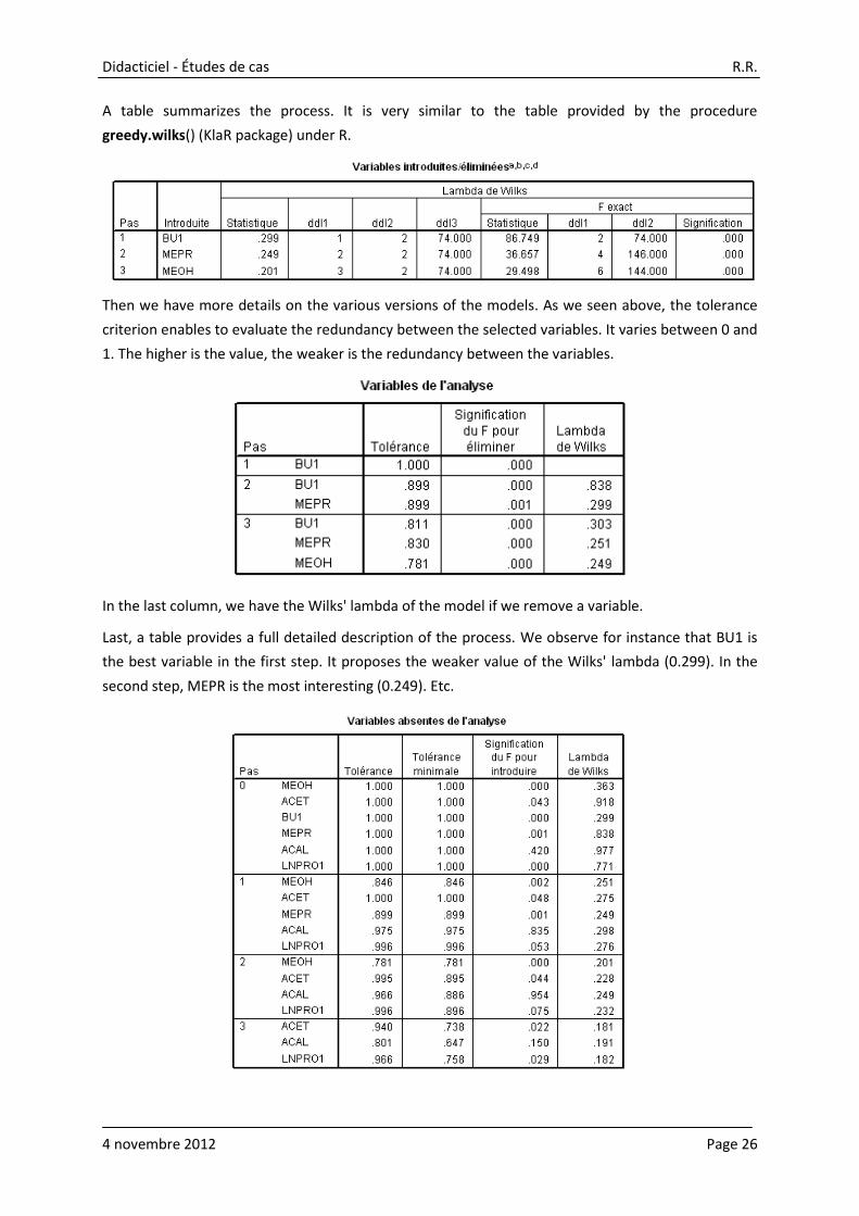
A table summarizes the process. It is very similar to the table provided by the procedure
greedy.wilks() (KlaR package) under R.
Then we have more details on the various versions of the models. As we seen above, the tolerance
criterion enables to evaluate the redundancy between the selected variables. It varies between 0 and
1. The higher is the value, the weaker is the redundancy between the variables.
In the last column, we have the Wilks' lambda of the model if we remove a variable.
Last, a table provides a full detailed description of the process. We observe for instance that BU1 is
the best variable in the first step. It proposes the weaker value of the Wilks' lambda (0.299). In the
second step, MEPR is the most interesting (0.249). Etc.

Didacticiel - Études de cas R.R.
4 novembre 2012 Page 27
7 Conclusion
Discriminant analysis is an attractive method. It is available in almost all statistical software. In this
tutorial, we tried to highlight the similarities and the differences between the outputs of Tanagra, R,
SAS, and SPSS software. The main conclusion is that, if the presentation is not always the same,
ultimately we have exactly the same results. This is the most important.