arX

iv:1

904.

0491

9v2

[ph

ysic

s.fl

u-dy

n] 1

1 A

pr 2

019

This draft was prepared using the LaTeX style file belonging to the Journal of Fluid Mechanics.To appear in Journal of Fluid Mechanics

1

Analytic Reconstruction of aTwo-Dimensional Velocity Field from an

Observed Diffusive Scalar

Arjun Sharma1, Irina I. Rypina 2, Ruth Musgrave2 and GeorgeHaller1†

1Institute for Mechanical Systems, ETH Zurich, Leonhardstrasse 21, 8092 Zurich, Switzerland2Woods Hole Oceanographic Institution, 266 Woods Hole rd., Woods Hole, MA 02543, USA

(Received xx; revised xx; accepted xx)

Inverting an evolving diffusive scalar field to reconstruct the underlying velocity fieldis an underdetermined problem. Here we show, however, that for two-dimensional in-compressible flows, this inverse problem can still be uniquely solved if high-resolutiontracer measurements, as well as velocity measurements along a curve transverse to theinstantaneous scalar contours, are available. Such measurements enable solving a systemof partial differential equations for the velocity components by the method of character-istics. If the value of the scalar diffusivity is known, then knowledge of just one velocitycomponent along a transverse initial curve is sufficient. These conclusions extend to theshallow-water equations and to flows with spatially dependent diffusivity. We illustrateour results on velocity reconstruction from tracer fields for planar Navier–Stokes flows andfor a barotropic ocean circulation model. We also discuss the use of the proposed velocityreconstruction in oceanographic applications to extend localised velocity measurementsto larger spatial domains with the help of remotely sensed scalar fields.

1. Introduction and related work

The measurement of an evolving scalar tracer is sometimes considered easier thanthat of the underlying velocity (Schlichtholz 1991), both in nature and in a laboratorysetting. Determining the flow velocity more accurately from scalar field observations is,therefore, an exciting perspective in a plethora of applications including oceanography,meteorology, medicine and chemical engineering (Wunsch 1987).The transport equation for a passive scalar with instantaneous concentration c(x, t)

and constant diffusivity µ > 0 under an incompressible, planar velocity field u(x, t) isgiven by

∂c

∂t+ u · ∇c = µ∇2c, (1.1)

with the spatial coordinates x = (x, y) varying over some domain U ⊂ R2 and t denoting

the time. Note that the velocity field u only influences the advection of c via its innerproduct u · ∇c with the instantaneous concentration gradient. This leads to the classicobservation that the iso-scalar component of the velocity is inconsequential for the scalarfield evolution (Dahm et al. 1992; Kelly 1989). In other words, the iso-scalar velocitycomponent falls in the null space of the velocity-reconstruction problem, necessitatingfurther conditions for a unique solution to this inverse problem (Kelly 1989).Seminal work by Fiadeiro & Veronis (1984) and Wunsch (1985) considered velocity

† Email address for correspondence: georgehaller@ethz.ch

2 Sharma et al.

reconstruction from discretized observations of a steady scalar distribution in a two-dimensional, steady channel flow with uniform velocity. After spatial discretization, theseauthors obtained an under-determined algebraic system of equations for the values ofthe streamfunction at the grid points. The minimum-norm solution obtained to thisproblem by Fiadeiro & Veronis (1984) and Wunsch (1985) was found to be qualitativelyinaccurate by Veronis (1986) even for the simple uniform flow considered. Providingadditional boundary conditions (Fiadeiro & Veronis 1984) or information on the flowanisotropy (Wunsch 1985) leads to improved solutions. Alternatively, if the flow isdispensed with two scalars of different diffusivity, the system becomes over-determinedbecause the same streamfunction must satisfy two linearly independent scalar equations.This reformulation, however, allows for a physically realistic solution that minimizes theleast-squares of the solution error, as obtained by Fiadeiro & Veronis (1984). As expected,the reconstructed velocity departs from the true velocity significantly in regions wherethe two scalar fields are similarly distributed.

An alternative approach to inverting the scalar transport equation (1.1) has led tothe emergence of Scalar Imaging Velocimetry (SIV) (see Wallace & Vukoslavcevic 2010for a review). When the diffusion of the scalar is slower than that of the carrier fluid(i.e., the ratio of fluid viscosity and scalar diffusivities is larger than one), the fluidvelocity at nearby points varies slower than the scalar intensity (Dahm et al. 1992). Asa consequence, the velocity component normal to the iso-scalar varies faster than theoverall velocity. For an initial estimate, the overall velocity can therefore be assumedlocally spatially constant and recovered from a projection onto neighboring normals toiso-scalar curves. As the calculation of iso-scalar-normal velocity requires division by|∇c|, the velocity reconstructed in this fashion is limited to regions where |∇c| is wellseparated from zero (Dahm et al. 1992).

In an another approach relaxing the requirement of slow scalar diffusion, Su & Dahm(1996) formulated the velocity reconstruction as a minimization problem for an integralcomposed of the transport equation, the divergence and a regularizer term dependingon the velocity gradient norm. Kelly (1989) also implemented a similar formulation forocean flows in which the functional to be minimized involves the transport equation, thehorizontal divergence, the relative vorticity and the kinetic energy. These minimizationtechniques can return an accurate (albeit never exact) velocity field if the weight factorsfor each component of the functional are tuned appropriately.

Here, we point out that for two-dimensional incompressible flows, one can use themethod of characteristics to analytically reformulate the partial differential equation(PDE) (1.1) into a system of ordinary differential equations (ODEs) for the spatialevolution of the velocity components along an instantaneous level curve of c(x, t).Integration of these ODEs enables the reconstruction of the velocity field over the domainof scalar observations. This procedure assumes that the velocity is available along a curveΓ (t) transverse to the level curves of c(x, t). If the value of the diffusivity µ is known,knowledge of one velocity component along Γ (t) turns out to be sufficient. We give thederivation of these results in section 2 and test the approach on two numerical examplesin section 3.

Our technique can be particularly advantageous in oceanographic applications, inwhich often only localised velocity field measurements are available. In such situations,independent observations of larger-scale physical, chemical or biological tracer fields offeran opportunity to extend the local velocity data to larger domains, as we illustratein section 4. We also discuss oceanography-inspired extensions of our main results todiffusivities with spatial dependence and to shallow-water equations in section 2.

Velocity from scalar field 3

2. Formulation

Taking the spatial gradient of the scalar transport equation (1.1) leads to the equations

∂2c

∂t∂x+ u

∂2c

∂x2+∂u

∂x

∂c

∂x+ v

∂2c

∂x∂y+∂v

∂x

∂c

∂y= µ

∂∇2c

∂x, (2.1a)

∂2c

∂t∂y+ u

∂2c

∂x∂y+∂u

∂y

∂c

∂x+ v

∂2c

∂y2+∂v

∂y

∂c

∂y= µ

∂∇2c

∂y. (2.1b)

There is no general recipe for solving such a coupled system of linear PDEs. Remarkably,however, the incompressibility condition

∂u

∂x+∂v

∂y= 0 (2.2)

enables us to rewrite this system as

∂v

∂x

∂c

∂y− ∂v

∂y

∂c

∂x= −u ∂

2c

∂x2− v

∂2c

∂x∂y− ∂2c

∂t∂x+ µ

∂∇2c

∂x, (2.3a)

∂u

∂x

∂c

∂y− ∂u

∂y

∂c

∂x= u

∂2c

∂x∂y+ v

∂2c

∂y2+

∂2c

∂t∂y− µ

∂∇2c

∂y. (2.3b)

Both equations in system (2.3) share the same characteristics x(s; t) = (x(s; t), y(s; t)),which satisfy the system of ODEs

dx(s; t)

ds=∂c(x(s; t), t)

∂y,

dy(s; t)

ds= −∂c(x(s; t), t)

∂x, (2.4)

with the instantaneous time t playing the role of a parameter. These characteristics arepointwise normal to the gradient ∇c and hence coincide with instantaneous level curvesof c(x, t) at any time t. Along the characteristics (2.4), the PDEs in (2.3) can be re-written as a linear, two-dimensional, non-autonomous system of ODEs for the velocityu(s; t) := u(x(s; t), t). This ODE is of the form

du(s; t)

ds= A(s; t)u(s; t) + b(s; t), u(s; t) ∈ R

2, s ∈ R, (2.5)

with the form of the matrix A(s; t) ∈ R2×2 and the vector b(s; t) ∈ R

2 depending uponwether the constant scalar diffusivity, µ, is known or unknown, as we discuss belowseparately. In either case, once the normalized fundamental matrix solution Φ(s; t) of thehomogenous part du

ds= A(s; t)u, satisfying Φ(0; t) = I, has been numerically determined,

we can integrate (2.5) directly to obtain the velocity

u(s; t) = Φ(s; t)u(0; t) +

∫ s

0

Φ(s− σ; t)b(σ; t)dσ (2.6)

at any location x(s; t) along the level curve of c(x, t) containing the point x(0; t).

2.1. Case of known scalar diffusivity

In the case where the value of µ is a priori known, equations (2.3) can be recast in theform (2.5) with the help of

A(s; t) =

[

∂2c∂x∂y

∂2c∂y2

− ∂2c∂x2 − ∂2c

∂x∂y

]

x=x(s;t)

, b(s; t) =

[

∂2c∂t∂y

− µ∂∇2c∂y

− ∂2c∂t∂x

+ µ∂∇2c∂x

]

x=x(s;t)

. (2.7)

4 Sharma et al.

2.2. Case of unknown scalar diffusivity

If the value of µ is a priori unknown, we can still express µ from the original transportequation (1.1) as

µ =1

∇2c

(∂c

∂t+ u

∂c

∂x+ v

∂c

∂y

)

. (2.8)

Substitution of this expression into (2.3) enables us to rewrite (2.3) in the form (2.5)with

A(s; t) =

[

∂2c∂x∂y

− 1∇2c

∂c∂x

∂∇2c∂y

∂2c∂y2 − 1

∇2c∂c∂y

∂∇2c∂y

− ∂2c∂x2 + 1

∇2c∂c∂x

∂∇2c∂x

− ∂2c∂x∂y

+ 1∇2c

∂c∂y

∂∇2c∂x

]

x=x(s;t)

,

b(s; t) =

[

∂2c∂t∂y

− 1∇2c

∂c∂t

∂∇2c∂y

− ∂2c∂t∂x

+ 1∇2c

∂c∂t

∂∇2c∂x

]

x=x(s;t)

.

(2.9)

The formulae in equation (2.9), however, are only well-defined at points where ∇2c 6= 0.

2.3. Spatially-dependent diffusivity

Most non-eddy-resolving ocean circulation models are diffusion-based, i.e., assumethat the small-scale, un- and under-resolved eddy motions lead to a diffusive tracertransfer—a process that can be fully characterized by just one parameter, the lateral eddydiffusivity µ. A number of diffusivity estimates are available based on data from surfacedrifters and tracers (Okubo 1971; Zhurbas & Oh 2004; LaCasce 2008; Rypina et al. 2012;LaCasce & Bower 2000; Lumpkin et al. 2002; McClean et al. 2002) satellite-observed ve-locity fields (Marshall et al. 2006; Abernathey & Marshall 2013; Klocker & Abernathey2014; Rypina et al. 2012) and Argo float observations (Cole et al. 2015). All these obser-vations suggest that the ocean eddy diffusivity is strongly spatially varying with up totwo orders of magnitude difference between regions with quiescent vs. energetic oceaniceddy regimes. Eddy-resolving simulations also demonstrate highly nonuniform spatialdistribution of the eddy-induced transport (Gille & Davis 1999; Nakamura & Chao 2000;Roberts & Marshall 2000). Thus, any method that involves diffusivity assumption in aglobal settings, including the velocity reconstruction method described here, would needto take into account spatial variation in diffusivity.In this case, the appropriate advection-diffusion equation takes the form

∂c

∂t+ u · ∇c = ∇(µ∇c). (2.10)

Taking the gradient of this equation and following the same steps as in Section 2,one obtains that the velocity u satisfies equation (2.5) along the iso-curves of tracerconcentration c, with A from eq. (2.7) and

b(s; t) =

[

∂2c∂t∂y

− ∂∇(µ∇c)∂y

− ∂2c∂t∂x

+ ∂∇(µ∇c)∂x

]

x=x(s;t)

. (2.11)

2.4. Shallow-water approximation

Due to negligible vertical velocities, eq. (2.2) is a reasonable approximation for oceanicsurface flows on spatial scales larger than the mesoscale (Pedlosky 2013; Salmon 1998;Bennett 2005). When vertical velocities become non-negligible, one may still find anothervariable other than the velocity that satisfies eq. (2.2) and re-derive the inversion forthat variable. An example is the inviscid shallow-water model with a rigid lid (Pedlosky

Velocity from scalar field 5

2013; Batchelor 1967), as we shall discuss next. This shallow-water approximation is oftenemployed in physical oceanography to describe ocean flows in shallow tidally-driven bays,such as, for example, the Katama Bay located on the island of Martha’s Vineyard, MA(Slivinski et al. 2017; Orescanin et al. 2016; Luettich Jr & Westerink 1991).Consider a shallow sheet of inviscid unstratified fluid overlaying spatially-dependent

bathymetry. Fluid parcels are allowed to have three non-zero components of velocity,{u, v, w} 6= 0, but if the horizontal velocity u is initially independent of z then it remainsso for all times, i.e., we may write

u = u(x, y, t). (2.12)

If the initial tracer distribution is independent of z, i.e., c0 = c0(x, y), then we will alsohave

c = c(x, y, t) (2.13)

for all times. We then invoke a rigid-lid approximation, assuming that the free surfaceelevation η—the deviation of the free surface from its mean value—is much smaller thanthe water depth h(x, y), i.e., η ≪ h≪ L, where L is the characteristic horizontal lengthscale of motion. Then the water depth is time-independent and can be considered knownbecause the bathymetry of a shallow bay can be mapped out and the sea surface heightis assumed to be constant due to the rigid lid approximation.In this case, mass conservation requires the transport velocity, hu, to be divergence

free:

∂(hu)/∂x+ ∂(hv)/∂y = 0. (2.14)

To proceed, we multiply the advection- diffusion equation (2.10) by h to obtain

h∂c

∂t+ hu · ∇c = h∇(µ∇c). (2.15)

We take the gradient of this equation, then follow the steps of section 2 to obtain ananalogue of eq. (2.5) for the transport velocity, given by

d(hu)/ds = A(hu) + b, (2.16)

with A from eq. (2.7) and with

b(s; t) =

[

∂∂y

(h ∂c∂y

)− ∂∂y

(h∇(µ∇c))− ∂

∂x(h ∂c

∂y) + ∂

∂x(h∇(µ∇c))

]

x=x(s;t)

. (2.17)

As before, equation (2.16) should be solved along the iso-contours of c, which are thecharacteristics of the PDE (2.15).

2.5. Velocity reconstruction

For an experimentally or numerically obtained scalar field, c(x, t), the characteristicx(s; t) emanating from any point x0(t) := x(0; t) can be computed numerically fromequation (2.4). To recover the velocity u(s; t) at a point x(s; t) of such a characteristicvia (2.6), we need to know the velocity u(0; t) at the initial location x0(t). The PDE(2.3) is well-posed only if such a set of initial velocity vectors is available along anon-characteristic curve Γ (t), i.e., along a curve segment that is transverse to thecharacteristics at each of its points. If, however, the diffusivity µ is a priori available, thenonly one component of u(0; t) = u(x0, t) needs to be known along the non-characteristiccurve Γ (t), because the other component can be determined from (1.1). For example, ifonly the u(x, t) velocity is known at a point of x ∈ Γ (t), then v(x, t) can be uniquely

6 Sharma et al.

determined from (1.1) as long as the contour of c(x, t) is not locally parallel to the xdirection, i.e., as long as ∂c(x, t)/∂y 6= 0.To reconstruct the velocity field u(x, t) over the largest possible domain, the initial

velocities must therefore be known along a curve Γ (t) transverse to the level curvesof c(x, t) over the largest possible domain. Most of the characteristics (level curves)in our examples will be closed, but this is not a requirement for our method to beapplicable. Indeed, to obtain u(x, t) along a non-closed level set of c(x, t), one simply hasto integrate equation (2.4) both in the forward and the backward s-direction until thedomain boundary is reached.The formulae (2.7)-(2.17) contain the first-order temporal derivative of the observed

scalar c(x, t), as well as up to second and up to third-order spatial derivatives, respec-tively. This presents challenges for velocity reconstruction over domains where onlyscarce information is available on c(x, t). We envision, however, applications of thisvelocity reconstruction procedure in situations where high-resolution imaging of c(x, t)is available, enabling an accurate computation of the necessary derivatives.In geophysical flows, the ratio of advective transport rate to the diffusive rate (i.e.

the dimensionless Peclet number) tends to be large. For such large Peclet numbers,in the formulae relevant for velocity reconstruction under a known diffusivity (eqs.(2.7), (2.9), (2.11) and (2.17)), errors and uncertainties arising from computing thenecessary third derivatives are suppressed by the small µ values multiplying these terms.We illustrate this effect in section 4.2 with respect to substantial under-sampling andmoderate uncertainties.

3. Numerical examples

We now carry out our proposed velocity reconstruction scheme in two examples. Inboth, we generate c(x, t) numerically by evolving an initial scalar distribution c0(x) :=c(x, t0) under the PDE (1.1) with a known velocity field u(x, t), then reconstruct u(x, t)solely from observations of c(x, t). We solve for c(x, t) by discretizing (1.1) using thepseudospectral method. The necessary spatial derivatives of c(x, t) in the reconstructionformulae are evaluated in the frequency domain using MATLAB’s FFT algorithm; thetime integration is performed in real space using MATLAB’s variable-order adaptivetime step solver, ODE45. The standard 2/3 dealiasing is applied where the energy inthe last one third of the wavenumbers is artificially removed. In both examples, thescalar diffusivity is taken to be µ = 0.01 and a 512 × 512 grid is used. We performthe integration of the characteristic ODEs (equations (2.4) and (2.5)) using MATLAB’sODE113 to achieve high accuracy.

3.1. Example 1: Steady, analytic, inviscid velocity field

We consider the Mallier–Maslowe vortices (Mallier & Maslowe 1993; Gurarie & Chow2004) which are exact solutions of the 2D Euler equations. Modeling a periodic row ofvortices with alternating rotation directions, the corresponding velocity field derives fromthe streamfunction

ψ(x) = arctanh[ α cos

√1 + α2x√

1 + α2 coshαy

]

, (3.1)

which we plot for reference in the left panel of figure 1 for α = 1.Over the square domain x ∈ [0, 2

√2π]× [−

√2π,

√2π], we generate the diffusive scalar

distribution c(x, t) from the initial concentration field c(x, 0) = 4 exp[−0.2((x−√2π)2 +

y2)] by solving the transport equation (1.1). No advective transport is possible among

Velocity from scalar field 7

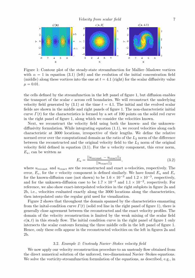
Figure 1: Contour plot of the steady-state streamfunction for Mallier–Maslowe vorticeswith α = 1 in equation (3.1) (left) and the evolution of the initial concentration field(middle) along these vortices into the one at t = 4.1 (right) for the scalar diffusivity valueµ = 0.01.

the cells defined by the streamfunction in the left panel of figure 1, but diffusion enablesthe transport of the scalar c across cell boundaries. We will reconstruct the underlyingvelocity field generated by (3.1) at the time t = 4.1. The initial and the evolved scalarfields are shown in the middle and right panels of figure 1. The non-characteristic initialcurve Γ (t) for the characteristics is formed by a set of 100 points on the solid red curvein the right panel of figure 1, along which we consider the velocities known.Next, we reconstruct the velocity field using both the known- and the unknown-

diffusivity formulation. While integrating equation (1.1), we record velocities along eachcharacteristic at 3000 locations, irrespective of their lengths. We define the relativenormed error over the computational domain as the ratio of the L2 norm of the differencebetween the reconstructed and the original velocity field to the L2 norm of the originalvelocity field defined in equation (3.1). For the u velocity component, this error norm,Eu, can be written as

Eu =||ureconst. − uexact||2

||uexact||2, (3.2)

where ureconst. and uexact are the reconstructed and exact u-velocities, respectively. Theerror, Ev, for the v velocity component is defined similarly. We have found Eu and Ev

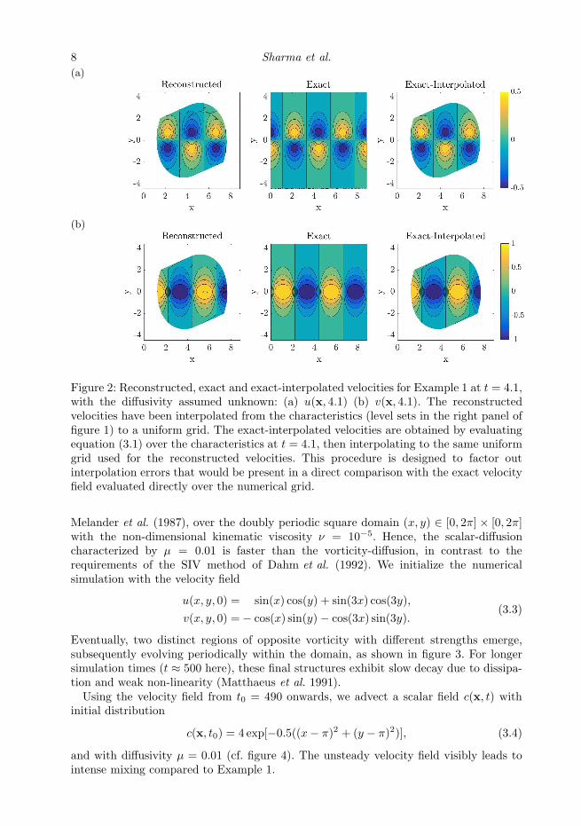
for the known-diffusion case (not shown) to be 1.6 × 10−3 and 1.2 × 10−3, respectively,and for the unknown-diffusion case to be 1.7 × 10−2 and 1.1 × 10−2, respectively. Forreference, we also show exact-interpolated velocities in the right subplots in figure 2a and2b, i.e., velocities evaluated exactly along the 3000 locations along the characteristics,then interpolated onto the regular grid used for visualization.Figure 2 shows that throughout the domain spanned by the characteristics emanating

from the inital-condition curve Γ (t) (solid red line in the right panel of figure 1), there isgenerally close agreement between the reconstructed and the exact velocity profiles. Thedomain of the velocity reconstruction is limited by the weak mixing of the scalar fieldc(x, t) in this steady flow. The initial condition curve in the right panel of figure 1 onlyintersects the scalar contours forming the three middle cells in the left panel of figure 1.Hence, only these cells appear in the reconstructed velocities on the left in figures 2a and2b.

3.2. Example 2: Unsteady Navier–Stokes velocity field

We now apply our velocity reconstruction procedure to an unsteady flow obtained fromthe direct numerical solution of the unforced, two-dimensional Navier–Stokes equations.We solve the vorticity-streamfunction formulation of the equations, as described, e.g., in

8 Sharma et al.

(a)

(b)

Figure 2: Reconstructed, exact and exact-interpolated velocities for Example 1 at t = 4.1,with the diffusivity assumed unknown: (a) u(x, 4.1) (b) v(x, 4.1). The reconstructedvelocities have been interpolated from the characteristics (level sets in the right panel offigure 1) to a uniform grid. The exact-interpolated velocities are obtained by evaluatingequation (3.1) over the characteristics at t = 4.1, then interpolating to the same uniformgrid used for the reconstructed velocities. This procedure is designed to factor outinterpolation errors that would be present in a direct comparison with the exact velocityfield evaluated directly over the numerical grid.

Melander et al. (1987), over the doubly periodic square domain (x, y) ∈ [0, 2π] × [0, 2π]with the non-dimensional kinematic viscosity ν = 10−5. Hence, the scalar-diffusioncharacterized by µ = 0.01 is faster than the vorticity-diffusion, in contrast to therequirements of the SIV method of Dahm et al. (1992). We initialize the numericalsimulation with the velocity field

u(x, y, 0) = sin(x) cos(y) + sin(3x) cos(3y),

v(x, y, 0) =− cos(x) sin(y)− cos(3x) sin(3y).(3.3)

Eventually, two distinct regions of opposite vorticity with different strengths emerge,subsequently evolving periodically within the domain, as shown in figure 3. For longersimulation times (t ≈ 500 here), these final structures exhibit slow decay due to dissipa-tion and weak non-linearity (Matthaeus et al. 1991).Using the velocity field from t0 = 490 onwards, we advect a scalar field c(x, t) with

initial distribution

c(x, t0) = 4 exp[−0.5((x− π)2 + (y − π)2)], (3.4)

and with diffusivity µ = 0.01 (cf. figure 4). The unsteady velocity field visibly leads tointense mixing compared to Example 1.

Velocity from scalar field 9

(a) (b)

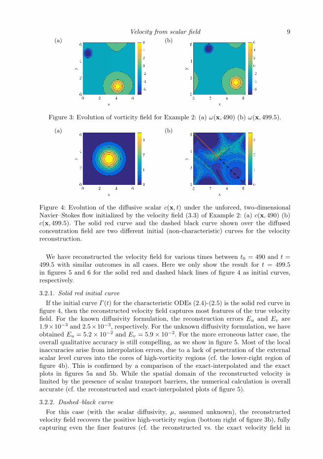
Figure 3: Evolution of vorticity field for Example 2: (a) ω(x, 490) (b) ω(x, 499.5).

(a) (b)

Figure 4: Evolution of the diffusive scalar c(x, t) under the unforced, two-dimensionalNavier–Stokes flow initialized by the velocity field (3.3) of Example 2: (a) c(x, 490) (b)c(x, 499.5). The solid red curve and the dashed black curve shown over the diffusedconcentration field are two different initial (non-characteristic) curves for the velocityreconstruction.

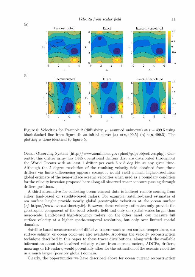
We have reconstructed the velocity field for various times between t0 = 490 and t =499.5 with similar outcomes in all cases. Here we only show the result for t = 499.5in figures 5 and 6 for the solid red and dashed black lines of figure 4 as initial curves,respectively.

3.2.1. Solid red initial curve

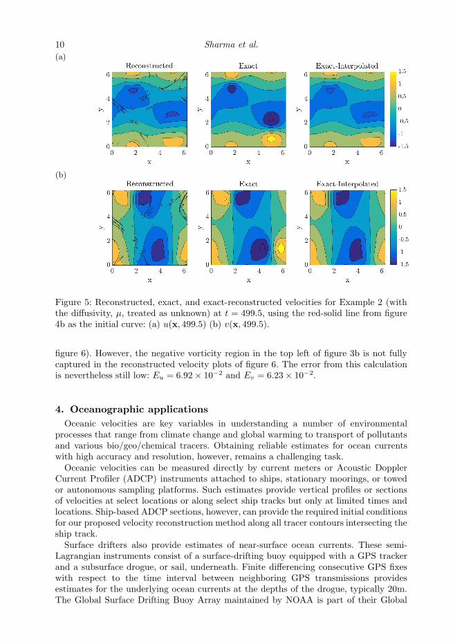
If the initial curve Γ (t) for the characteristic ODEs (2.4)-(2.5) is the solid red curve infigure 4, then the reconstructed velocity field captures most features of the true velocityfield. For the known diffusivity formulation, the reconstruction errors Eu and Ev are1.9×10−3 and 2.5×10−3, respectively. For the unknown diffusivity formulation, we haveobtained Eu = 5.2× 10−2 and Ev = 5.9× 10−2. For the more erroneous latter case, theoverall qualitative accuracy is still compelling, as we show in figure 5. Most of the localinaccuracies arise from interpolation errors, due to a lack of penetration of the externalscalar level curves into the cores of high-vorticity regions (cf. the lower-right region offigure 4b). This is confirmed by a comparison of the exact-interpolated and the exactplots in figures 5a and 5b. While the spatial domain of the reconstructed velocity islimited by the presence of scalar transport barriers, the numerical calculation is overallaccurate (cf. the reconstructed and exact-interpolated plots of figure 5).

3.2.2. Dashed–black curve

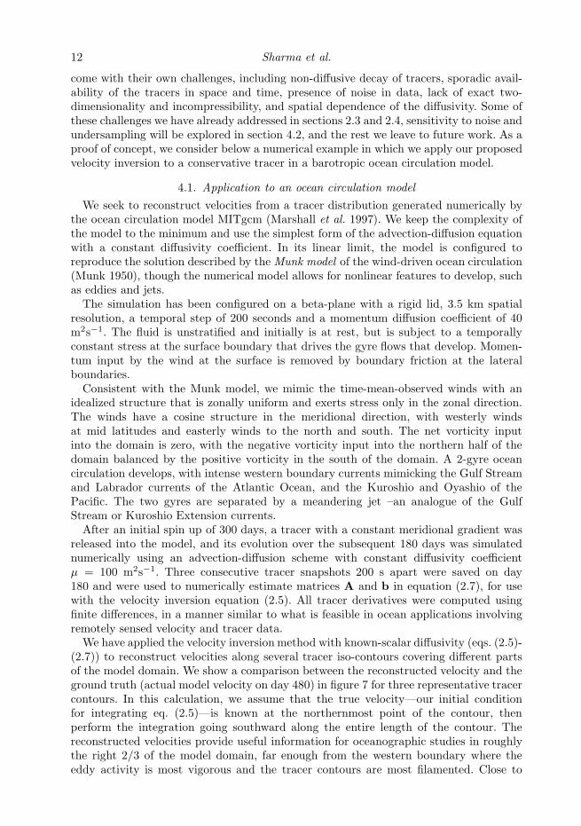
For this case (with the scalar diffusivity, µ, assumed unknown), the reconstructedvelocity field recovers the positive high-vorticity region (bottom right of figure 3b), fullycapturing even the finer features (cf. the reconstructed vs. the exact velocity field in

10 Sharma et al.

(a)

(b)

Figure 5: Reconstructed, exact, and exact-reconstructed velocities for Example 2 (withthe diffusivity, µ, treated as unknown) at t = 499.5, using the red-solid line from figure4b as the initial curve: (a) u(x, 499.5) (b) v(x, 499.5).

figure 6). However, the negative vorticity region in the top left of figure 3b is not fullycaptured in the reconstructed velocity plots of figure 6. The error from this calculationis nevertheless still low: Eu = 6.92× 10−2 and Ev = 6.23× 10−2.

4. Oceanographic applications

Oceanic velocities are key variables in understanding a number of environmentalprocesses that range from climate change and global warming to transport of pollutantsand various bio/geo/chemical tracers. Obtaining reliable estimates for ocean currentswith high accuracy and resolution, however, remains a challenging task.Oceanic velocities can be measured directly by current meters or Acoustic Doppler

Current Profiler (ADCP) instruments attached to ships, stationary moorings, or towedor autonomous sampling platforms. Such estimates provide vertical profiles or sectionsof velocities at select locations or along select ship tracks but only at limited times andlocations. Ship-based ADCP sections, however, can provide the required initial conditionsfor our proposed velocity reconstruction method along all tracer contours intersecting theship track.Surface drifters also provide estimates of near-surface ocean currents. These semi-

Lagrangian instruments consist of a surface-drifting buoy equipped with a GPS trackerand a subsurface drogue, or sail, underneath. Finite differencing consecutive GPS fixeswith respect to the time interval between neighboring GPS transmissions providesestimates for the underlying ocean currents at the depths of the drogue, typically 20m.The Global Surface Drifting Buoy Array maintained by NOAA is part of their Global

Velocity from scalar field 11

(a)

(b)

Figure 6: Velocities for Example 2 (diffusivity, µ, assumed unknown) at t = 499.5 usingblack-dashed line from figure 4b as initial curve: (a) u(x, 499.5) (b) v(x, 499.5). Theplotting is done identical to figure 5.

Ocean Observing System (http://www.aoml.noaa.gov/phod/gdp/objectives.php). Cur-rently, this drifter array has 1445 operational drifters that are distributed throughoutthe World Oceans with at least 1 drifter per each 5 x 5 deg bin at any given time.Although the 5 degree resolution of the resulting velocity field obtained from thesedrifters via finite differencing appears coarse, it would yield a much higher-resolutionglobal estimate of the near-surface oceanic velocities when used as a boundary conditionfor the velocity inversion proposed here along all observed tracer contours passing throughdrifters positions.A third alternative for collecting ocean current data is indirect remote sensing from

either land-based or satellite-based radars. For example, satellite-based estimates ofsea surface height provide nearly global geostrophic velocities at the ocean surface(cf. https://www.aviso.altimetry.fr). However, these velocity estimates only provide thegeostrophic component of the total velocity field and only on spatial scales larger thanmeso-scale. Land-based high-frequency radars, on the other hand, can measure fullsurface velocity at a higher spatio-temporal resolution, but only over limited spatialdomains.Satellite-based measurements of diffusive tracers–such as sea surface temperature, sea

surface salinity, or ocean color–are also available. Applying the velocity reconstructiontechnique described in this paper to these tracer distributions, along with the availableinformation about the localized velocity values from current meters, ADCPs, drifters,moorings or HF radars, would potentially allow for the estimation of the oceanic velocitiesin a much larger (possibly global) domain.Clearly, the opportunities we have described above for ocean current reconstruction

12 Sharma et al.

come with their own challenges, including non-diffusive decay of tracers, sporadic avail-ability of the tracers in space and time, presence of noise in data, lack of exact two-dimensionality and incompressibility, and spatial dependence of the diffusivity. Some ofthese challenges we have already addressed in sections 2.3 and 2.4, sensitivity to noise andundersampling will be explored in section 4.2, and the rest we leave to future work. As aproof of concept, we consider below a numerical example in which we apply our proposedvelocity inversion to a conservative tracer in a barotropic ocean circulation model.

4.1. Application to an ocean circulation model

We seek to reconstruct velocities from a tracer distribution generated numerically bythe ocean circulation model MITgcm (Marshall et al. 1997). We keep the complexity ofthe model to the minimum and use the simplest form of the advection-diffusion equationwith a constant diffusivity coefficient. In its linear limit, the model is configured toreproduce the solution described by the Munk model of the wind-driven ocean circulation(Munk 1950), though the numerical model allows for nonlinear features to develop, suchas eddies and jets.The simulation has been configured on a beta-plane with a rigid lid, 3.5 km spatial

resolution, a temporal step of 200 seconds and a momentum diffusion coefficient of 40m2s−1. The fluid is unstratified and initially is at rest, but is subject to a temporallyconstant stress at the surface boundary that drives the gyre flows that develop. Momen-tum input by the wind at the surface is removed by boundary friction at the lateralboundaries.Consistent with the Munk model, we mimic the time-mean-observed winds with an

idealized structure that is zonally uniform and exerts stress only in the zonal direction.The winds have a cosine structure in the meridional direction, with westerly windsat mid latitudes and easterly winds to the north and south. The net vorticity inputinto the domain is zero, with the negative vorticity input into the northern half of thedomain balanced by the positive vorticity in the south of the domain. A 2-gyre oceancirculation develops, with intense western boundary currents mimicking the Gulf Streamand Labrador currents of the Atlantic Ocean, and the Kuroshio and Oyashio of thePacific. The two gyres are separated by a meandering jet –an analogue of the GulfStream or Kuroshio Extension currents.After an initial spin up of 300 days, a tracer with a constant meridional gradient was

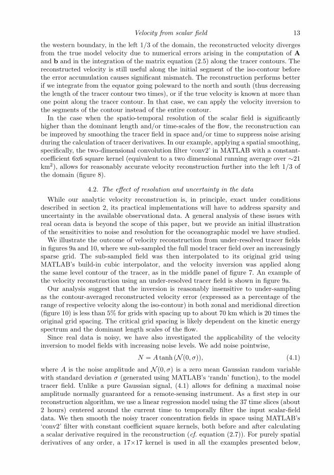
released into the model, and its evolution over the subsequent 180 days was simulatednumerically using an advection-diffusion scheme with constant diffusivity coefficientµ = 100 m2s−1. Three consecutive tracer snapshots 200 s apart were saved on day180 and were used to numerically estimate matrices A and b in equation (2.7), for usewith the velocity inversion equation (2.5). All tracer derivatives were computed usingfinite differences, in a manner similar to what is feasible in ocean applications involvingremotely sensed velocity and tracer data.We have applied the velocity inversion method with known-scalar diffusivity (eqs. (2.5)-

(2.7)) to reconstruct velocities along several tracer iso-contours covering different partsof the model domain. We show a comparison between the reconstructed velocity and theground truth (actual model velocity on day 480) in figure 7 for three representative tracercontours. In this calculation, we assume that the true velocity—our initial conditionfor integrating eq. (2.5)—is known at the northernmost point of the contour, thenperform the integration going southward along the entire length of the contour. Thereconstructed velocities provide useful information for oceanographic studies in roughlythe right 2/3 of the model domain, far enough from the western boundary where theeddy activity is most vigorous and the tracer contours are most filamented. Close to

Velocity from scalar field 13

the western boundary, in the left 1/3 of the domain, the reconstructed velocity divergesfrom the true model velocity due to numerical errors arising in the computation of Aand b and in the integration of the matrix equation (2.5) along the tracer contours. Thereconstructed velocity is still useful along the initial segment of the iso-contour beforethe error accumulation causes significant mismatch. The reconstruction performs betterif we integrate from the equator going poleward to the north and south (thus decreasingthe length of the tracer contour two times), or if the true velocity is known at more thanone point along the tracer contour. In that case, we can apply the velocity inversion tothe segments of the contour instead of the entire contour.In the case when the spatio-temporal resolution of the scalar field is significantly

higher than the dominant length and/or time-scales of the flow, the reconstruction canbe improved by smoothing the tracer field in space and/or time to suppress noise arisingduring the calculation of tracer derivatives. In our example, applying a spatial smoothing,specifically, the two-dimensional convolution filter ‘conv2’ in MATLAB with a constant-coefficient 6x6 square kernel (equivalent to a two dimensional running average over ∼21km2), allows for reasonably accurate velocity reconstruction further into the left 1/3 ofthe domain (figure 8).

4.2. The effect of resolution and uncertainty in the data

While our analytic velocity reconstruction is, in principle, exact under conditionsdescribed in section 2, its practical implementations will have to address sparsity anduncertainty in the available observational data. A general analysis of these issues withreal ocean data is beyond the scope of this paper, but we provide an initial illustrationof the sensitivities to noise and resolution for the oceanographic model we have studied.We illustrate the outcome of velocity reconstruction from under-resolved tracer fields

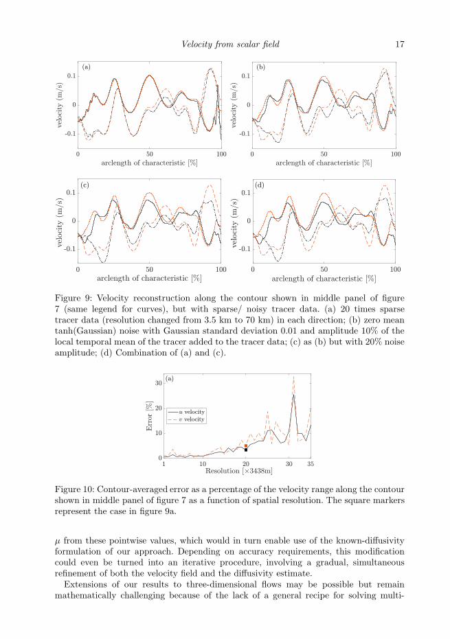
in figures 9a and 10, where we sub-sampled the full model tracer field over an increasinglysparse grid. The sub-sampled field was then interpolated to its original grid usingMATLAB’s build-in cubic interpolator, and the velocity inversion was applied alongthe same level contour of the tracer, as in the middle panel of figure 7. An example ofthe velocity reconstruction using an under-resolved tracer field is shown in figure 9a.Our analysis suggest that the inversion is reasonably insensitive to under-sampling

as the contour-averaged reconstructed velocity error (expressed as a percentage of therange of respective velocity along the iso-contour) in both zonal and meridional direction(figure 10) is less than 5% for grids with spacing up to about 70 km which is 20 times theoriginal grid spacing. The critical grid spacing is likely dependent on the kinetic energyspectrum and the dominant length scales of the flow.Since real data is noisy, we have also investigated the applicability of the velocity

inversion to model fields with increasing noise levels. We add noise pointwise,

N = A tanh (N (0, σ)), (4.1)

where A is the noise amplitude and N (0, σ) is a zero mean Gaussian random variablewith standard deviation σ (generated using MATLAB’s ‘randn’ function), to the modeltracer field. Unlike a pure Gaussian signal, (4.1) allows for defining a maximal noiseamplitude normally guaranteed for a remote-sensing instrument. As a first step in ourreconstruction algorithm, we use a linear regression model using the 37 time slices (about2 hours) centered around the current time to temporally filter the input scalar-fielddata. We then smooth the noisy tracer concentration fields in space using MATLAB’s‘conv2’ filter with constant coefficient square kernels, both before and after calculatinga scalar derivative required in the reconstruction (cf. equation (2.7)). For purely spatialderivatives of any order, a 17×17 kernel is used in all the examples presented below,

14 Sharma et al.

Figure 7: Right: Comparison between true and reconstructed u and v velocity componentsalong the 3 representative tracer iso-contours in an idealized model of the North AtlanticOcean. Left: Tracer distribution with the corresponding iso-contours.

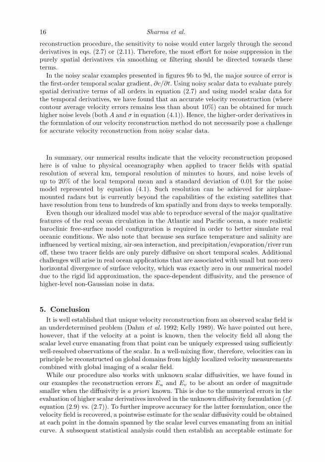
which correspond to about 58 km. The size of spatial filter for terms involving temporalderivatives is optimised for each case.Figure 9b shows the velocity reconstruction along the tracer contour in the middle

panel of 7 but using the noisy scalar data with noise amplitude A equal to 10% ofthe local temporal mean concentration across the 37 time slices (equivalent to a 2-hour period, which is effectively the observation time for this example) and setting astandard deviation σ equal to 0.01 in the definition (4.1). The shape of the iso-contour

Velocity from scalar field 15

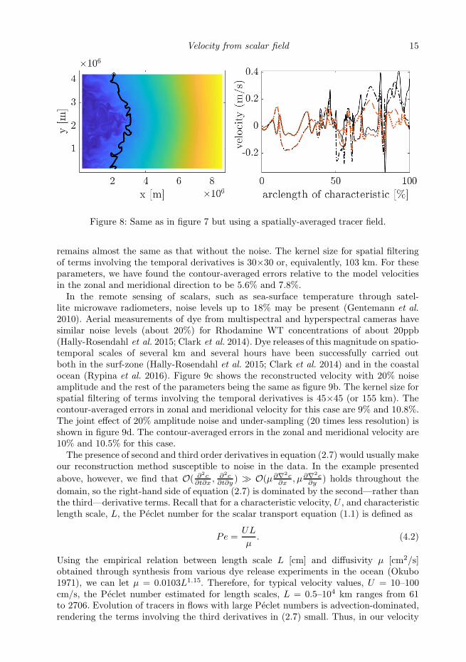
Figure 8: Same as in figure 7 but using a spatially-averaged tracer field.

remains almost the same as that without the noise. The kernel size for spatial filteringof terms involving the temporal derivatives is 30×30 or, equivalently, 103 km. For theseparameters, we have found the contour-averaged errors relative to the model velocitiesin the zonal and meridional direction to be 5.6% and 7.8%.In the remote sensing of scalars, such as sea-surface temperature through satel-

lite microwave radiometers, noise levels up to 18% may be present (Gentemann et al.

2010). Aerial measurements of dye from multispectral and hyperspectral cameras havesimilar noise levels (about 20%) for Rhodamine WT concentrations of about 20ppb(Hally-Rosendahl et al. 2015; Clark et al. 2014). Dye releases of this magnitude on spatio-temporal scales of several km and several hours have been successfully carried outboth in the surf-zone (Hally-Rosendahl et al. 2015; Clark et al. 2014) and in the coastalocean (Rypina et al. 2016). Figure 9c shows the reconstructed velocity with 20% noiseamplitude and the rest of the parameters being the same as figure 9b. The kernel size forspatial filtering of terms involving the temporal derivatives is 45×45 (or 155 km). Thecontour-averaged errors in zonal and meridional velocity for this case are 9% and 10.8%.The joint effect of 20% amplitude noise and under-sampling (20 times less resolution) isshown in figure 9d. The contour-averaged errors in the zonal and meridional velocity are10% and 10.5% for this case.The presence of second and third order derivatives in equation (2.7) would usually make

our reconstruction method susceptible to noise in the data. In the example presented

above, however, we find that O( ∂2c∂t∂x

, ∂2c∂t∂y

) ≫ O(µ∂∇2c∂x

, µ∂∇2c∂y

) holds throughout the

domain, so the right-hand side of equation (2.7) is dominated by the second—rather thanthe third—derivative terms. Recall that for a characteristic velocity, U , and characteristiclength scale, L, the Peclet number for the scalar transport equation (1.1) is defined as

Pe =UL

µ. (4.2)

Using the empirical relation between length scale L [cm] and diffusivity µ [cm2/s]obtained through synthesis from various dye release experiments in the ocean (Okubo1971), we can let µ = 0.0103L1.15. Therefore, for typical velocity values, U = 10–100cm/s, the Peclet number estimated for length scales, L = 0.5–104 km ranges from 61to 2706. Evolution of tracers in flows with large Peclet numbers is advection-dominated,rendering the terms involving the third derivatives in (2.7) small. Thus, in our velocity

16 Sharma et al.

reconstruction procedure, the sensitivity to noise would enter largely through the secondderivatives in eqs. (2.7) or (2.11). Therefore, the most effort for noise suppression in thepurely spatial derivatives via smoothing or filtering should be directed towards theseterms.In the noisy scalar examples presented in figures 9b to 9d, the major source of error is

the first-order temporal scalar gradient, ∂c/∂t. Using noisy scalar data to evaluate purelyspatial derivative terms of all orders in equation (2.7) and using model scalar data forthe temporal derivatives, we have found that an accurate velocity reconstruction (wherecontour average velocity errors remains less than about 10%) can be obtained for muchhigher noise levels (both A and σ in equation (4.1)). Hence, the higher-order derivatives inthe formulation of our velocity reconstruction method do not necessarily pose a challengefor accurate velocity reconstruction from noisy scalar data.

In summary, our numerical results indicate that the velocity reconstruction proposedhere is of value to physical oceanography when applied to tracer fields with spatialresolution of several km, temporal resolution of minutes to hours, and noise levels ofup to 20% of the local temporal mean and a standard deviation of 0.01 for the noisemodel represented by equation (4.1). Such resolution can be achieved for airplane-mounted radars but is currently beyond the capabilities of the existing satellites thathave resolution from tens to hundreds of km spatially and from days to weeks temporally.Even though our idealized model was able to reproduce several of the major qualitative

features of the real ocean circulation in the Atlantic and Pacific ocean, a more realisticbaroclinic free-surface model configuration is required in order to better simulate realoceanic conditions. We also note that because sea surface temperature and salinity areinfluenced by vertical mixing, air-sea interaction, and precipitation/evaporation/river runoff, these two tracer fields are only purely diffusive on short temporal scales. Additionalchallenges will arise in real ocean applications that are associated with small but non-zerohorizontal divergence of surface velocity, which was exactly zero in our numerical modeldue to the rigid lid approximation, the space-dependent diffusivity, and the presence ofhigher-level non-Gaussian noise in data.

5. Conclusion

It is well established that unique velocity reconstruction from an observed scalar field isan underdetermined problem (Dahm et al. 1992; Kelly 1989). We have pointed out here,however, that if the velocity at a point is known, then the velocity field all along thescalar level curve emanating from that point can be uniquely expressed using sufficientlywell-resolved observations of the scalar. In a well-mixing flow, therefore, velocities can inprinciple be reconstructed on global domains from highly localized velocity measurementscombined with global imaging of a scalar field.While our procedure also works with unknown scalar diffusivities, we have found in

our examples the reconstruction errors Eu and Ev to be about an order of magnitudesmaller when the diffusivity is a priori known. This is due to the numerical errors in theevaluation of higher scalar derivatives involved in the unknown diffusivity formulation (cf.equation (2.9) vs. (2.7)). To further improve accuracy for the latter formulation, once thevelocity field is recovered, a pointwise estimate for the scalar diffusivity could be obtainedat each point in the domain spanned by the scalar level curves emanating from an initialcurve. A subsequent statistical analysis could then establish an acceptable estimate for

Velocity from scalar field 17

Figure 9: Velocity reconstruction along the contour shown in middle panel of figure7 (same legend for curves), but with sparse/ noisy tracer data. (a) 20 times sparsetracer data (resolution changed from 3.5 km to 70 km) in each direction; (b) zero meantanh(Gaussian) noise with Gaussian standard deviation 0.01 and amplitude 10% of thelocal temporal mean of the tracer added to the tracer data; (c) as (b) but with 20% noiseamplitude; (d) Combination of (a) and (c).

Figure 10: Contour-averaged error as a percentage of the velocity range along the contourshown in middle panel of figure 7 as a function of spatial resolution. The square markersrepresent the case in figure 9a.

µ from these pointwise values, which would in turn enable use of the known-diffusivityformulation of our approach. Depending on accuracy requirements, this modificationcould even be turned into an iterative procedure, involving a gradual, simultaneousrefinement of both the velocity field and the diffusivity estimate.Extensions of our results to three-dimensional flows may be possible but remain

mathematically challenging because of the lack of a general recipe for solving multi-

18 Sharma et al.

dimensional systems of linear partial differential equations. An extension to generalcompressible flows appears beyond reach because incompressibility or specific form ofshallow water equations secures the common set of characteristic curves critical to ouranalytic solution strategy. A case with temporally constant but spatially varying densityof the fluid in 2D will have a similar formulation as the shallow water case.

The approach proposed here has the potential to extend spatially localized oceanvelocity measurements along contours of satellite-observed tracer fields, such as temper-ature, salinity and ocean color (phytoplankton) measurements. In Section 4, we haveprovided a first proof of concept by reconstructing larger-scale velocities generated bya global circulation model, with the tracer-field output of the same model serving asobservational input to our procedure. We have also demonstrated the robustness of thisreconstruction under sparsification of the observed scalar field and the addition of noisethat models observational inaccuracies. More work is required to investigate applicabilityof this method to real ocean data. Further work can build on the extension of our theorywe have given in sections 2.3-2.4 for spatially dependent diffusivities and 2D-divergentbut mass-conserving shallow water velocities.

We acknowledge useful conversations with Markus Holzner and Larry Pratt, as wellas partial funding from the Turbulent Superstructures priority program of the GermanNational Science Foundation (DFG), and from the NASA grant #NNX14AH29G to IR.

REFERENCES

Abernathey, Ryan Patrick & Marshall, J 2013 Global surface eddy diffusivities derivedfrom satellite altimetry. Journal of Geophysical Research: Oceans 118 (2), 901–916.

Batchelor, GK 1967 An introduction to fluid dynamics. Cambridge university press.Bennett, Andrew F 2005 Inverse modeling of the ocean and atmosphere. Cambridge

University Press.Clark, David B, Lenain, Luc, Feddersen, Falk, Boss, Emmanuel & Guza, RT 2014

Aerial imaging of fluorescent dye in the near shore. Journal of Atmospheric and OceanicTechnology 31 (6), 1410–1421.

Cole, Sylvia T, Wortham, Cimarron, Kunze, Eric & Owens, W Brechner 2015 Eddystirring and horizontal diffusivity from argo float observations: Geographic and depthvariability. Geophysical Research Letters 42 (10), 3989–3997.

Dahm, W. J., Su, L. K. & Southerland, K. B. 1992 A scalar imaging velocimetry techniquefor fully resolved four-dimensional vector velocity field measurements in turbulent flows.Physics of Fluids A: Fluid Dynamics 4 (10), 2191–2206.

Fiadeiro, M. E. & Veronis, G. 1984 Obtaining velocities from tracer distributions. Journalof Physical Oceanography 14 (11), 1734–1746.

Gentemann, Chelle L, Meissner, Thomas & Wentz, Frank J 2010 Accuracy of satellitesea surface temperatures at 7 and 11 ghz. IEEE Transactions on Geoscience and RemoteSensing 48 (3), 1009–1018.

Gille, Sarah T & Davis, Russ E 1999 The influence of mesoscale eddies on coarselyresolved density: An examination of subgrid-scale parameterization. Journal of physicaloceanography 29 (6), 1109–1123.

Gurarie, D. & Chow, K. W. 2004 Vortex arrays for sinh-Poisson equation of two-dimensionalfluids: Equilibria and stability. Physics of Fluids 16 (9), 3296–3305.

Hally-Rosendahl, Kai, Feddersen, Falk, Clark, David B & Guza, RT 2015 Surfzone toinner-shelf exchange estimated from dye tracer balances. Journal of Geophysical Research:Oceans 120 (9), 6289–6308.

Kelly, K. A. 1989 An inverse model for near-surface velocity from infrared images. Journal ofPhysical Oceanography 19 (12), 1845–1864.

Velocity from scalar field 19

Klocker, Andreas & Abernathey, Ryan 2014 Global patterns of mesoscale eddy propertiesand diffusivities. Journal of Physical Oceanography 44 (3), 1030–1046.

LaCasce, JHt 2008 Statistics from lagrangian observations. Progress in Oceanography 77 (1),1–29.

LaCasce, JH & Bower, A 2000 Relative dispersion in the subsurface north atlantic. Journalof marine research 58 (6), 863–894.

Luettich Jr, Richard A & Westerink, Joannes J 1991 A solution for the vertical variationof stress, rather than velocity, in a three-dimensional circulation model. InternationalJournal for Numerical Methods in Fluids 12 (10), 911–928.

Lumpkin, Rick, Treguier, Anne-Marie & Speer, Kevin 2002 Lagrangian eddy scales inthe northern atlantic ocean. Journal of physical oceanography 32 (9), 2425–2440.

Mallier, R. & Maslowe, S. A. 1993 A row of counter-rotating vortices. Physics of Fluids A:Fluid Dynamics (1989-1993) 5 (4), 1074–1075.

Marshall, John, Adcroft, Alistair, Hill, Chris, Perelman, Lev & Heisey, Curt 1997A finite-volume, incompressible navier stokes model for studies of the ocean on parallelcomputers. Journal of Geophysical Research: Oceans 102 (C3), 5753–5766.

Marshall, John, Shuckburgh, Emily, Jones, Helen & Hill, Chris 2006 Estimatesand implications of surface eddy diffusivity in the southern ocean derived from tracertransport. Journal of physical oceanography 36 (9), 1806–1821.

Matthaeus, W. H., Stribling, W. T., Martinez, D., Oughton, S. & Montgomery, D.1991 Decaying, two-dimensional, Navier-Stokes turbulence at very long times. Physica D:Nonlinear Phenomena 51 (1-3), 531–538.

McClean, Julie L, Poulain, Pierre-Marie, Pelton, Jimmy W & Maltrud, Mathew E2002 Eulerian and lagrangian statistics from surface drifters and a high-resolution popsimulation in the north atlantic. Journal of Physical Oceanography 32 (9), 2472–2491.

Melander, M. V., McWilliams, J. C. & Zabusky, N. J. 1987 Axisymmetrizationand vorticity-gradient intensification of an isolated two-dimensional vortex throughfilamentation. Journal of Fluid Mechanics 178, 137–159.

Munk, Walter H 1950 On the wind-driven ocean circulation. Journal of meteorology 7 (2),80–93.

Nakamura, Mototaka & Chao, Yi 2000 On the eddy isopycnal thickness diffusivity of thegent–mcwilliams subgrid mixing parameterization. Journal of climate 13 (2), 502–510.

Okubo, Akira 1971 Oceanic diffusion diagrams. In Deep sea research and oceanographicabstracts, , vol. 18, pp. 789–802. Elsevier.

Orescanin, Mara M, Elgar, Steve & Raubenheimer, Britt 2016 Changes in baycirculation in an evolving multiple inlet system. Continental Shelf Research 124, 13–22.

Pedlosky, Joseph 2013 Geophysical fluid dynamics. Springer Science & Business Media.

Roberts, Malcolm J & Marshall, David P 2000 On the validity of downgradient eddyclosures in ocean models. Journal of Geophysical Research: Oceans 105 (C12), 28613–28627.

Rypina, Irina I, Kamenkovich, Igor, Berloff, Pavel & Pratt, Lawrence J 2012Eddy-induced particle dispersion in the near-surface north atlantic. Journal of PhysicalOceanography 42 (12), 2206–2228.

Rypina, Irina I, Kirincich, A, Lentz, S & Sundermeyer, M 2016 Investigating the eddydiffusivity concept in the coastal ocean. Journal of Physical Oceanography 46 (7), 2201–2218.

Salmon, Rick 1998 Lectures on geophysical fluid dynamics. Oxford University Press.Schlichtholz, P. 1991 A review of methods for determining absolute velocities of water flow

from hydrographic data. Oceanologia 31, 73–85.Slivinski, LC, Pratt, Lawrence J, Rypina, Irina I, Orescanin, Mara M, Raubenheimer,

Britt, MacMahan, Jamie & Elgar, Steve 2017 Assimilating lagrangian data forparameter estimation in a multiple-inlet system. Ocean Modelling 113, 131–144.

Su, L. K. & Dahm, W. J. 1996 Scalar imaging velocimetry measurements of the velocitygradient tensor field in turbulent flows. i. Assessment of errors. Physics of Fluids 8 (7),1869–1882.

Veronis, G. 1986 Comments on “Can a tracer field be inverted for velocity?”. Journal ofPhysical Oceanography 16 (10), 1727–1730.

20 Sharma et al.

Wallace, J. M. & Vukoslavcevic, P. V. 2010 Measurement of the velocity gradient tensorin turbulent flows. Annual Review of Fluid Mechanics 42, 157–181.

Wunsch, C. 1985 Can a tracer field be inverted for velocity? Journal of Physical Oceanography15 (11), 1521–1531.

Wunsch, C. 1987 Using transient tracers: the regularization problem. Tellus B 39 (5), 477–492.Zhurbas, Victor & Oh, Im Sang 2004 Drifter-derived maps of lateral diffusivity in the pacific

and atlantic oceans in relation to surface circulation patterns. Journal of GeophysicalResearch: Oceans 109 (C5).