Embed Size (px)
Citation preview

1
The One-Sample t-TestAdapted from publically available slides attributed
to
Matthew Rockloff

2
When to use the one-sample t-test One of the most difficult aspects of
statistics is determining which procedure to use in what situation.
Mostly this is a matter of practice. There are many different rules of thumb
which may be of some help. In practice, however, the more you
understand the meaning behind each of the techniques, the more the choice will become obvious.
3
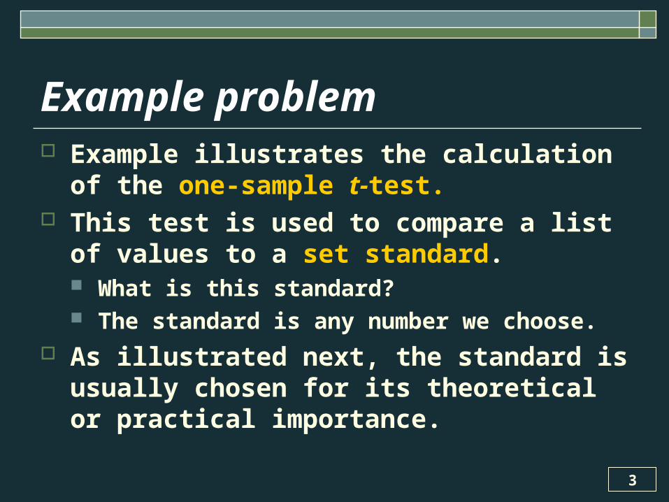
Example problem Example illustrates the calculation of
the one-sample t-test. This test is used to compare a list of
values to a set standard. What is this standard? The standard is any number we choose.
As illustrated next, the standard is usually chosen for its theoretical or practical importance.
4
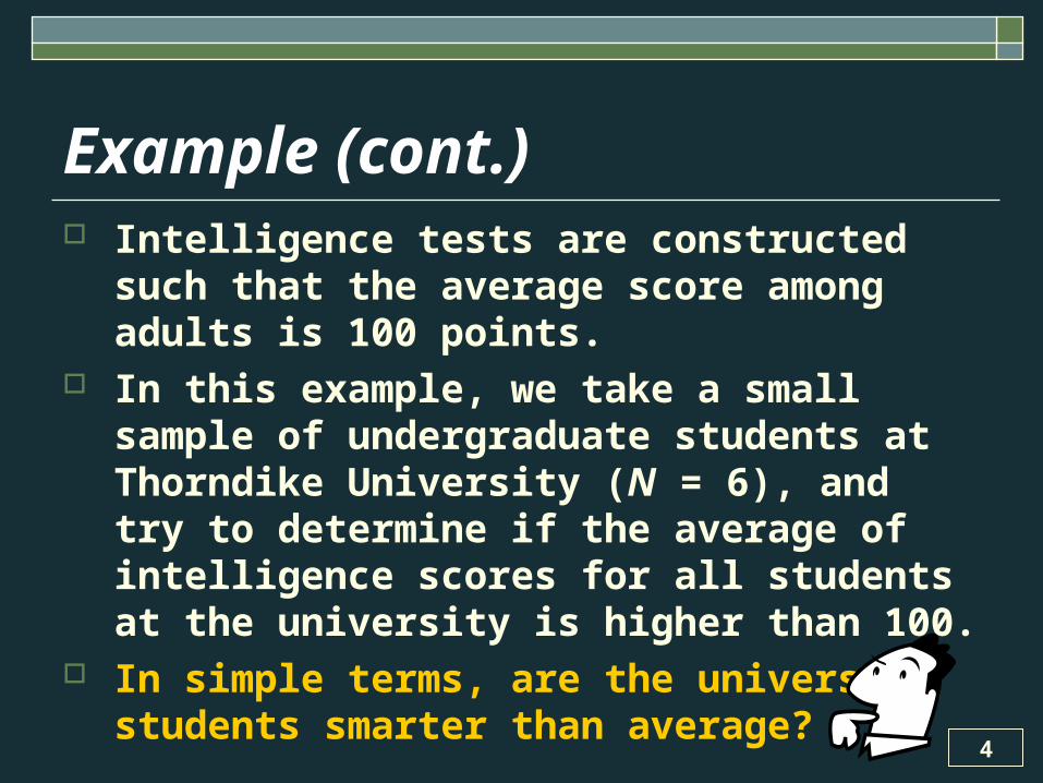
Example (cont.) Intelligence tests are constructed such that
the average score among adults is 100 points.
In this example, we take a small sample of undergraduate students at Thorndike University (N = 6), and try to determine if the average of intelligence scores for all students at the university is higher than 100.
In simple terms, are the university students smarter than average?

5
Example (cont.)
The scores obtained from the 6 students were as follows:
XPerson 1: 110Person 2: 118Person 3: 110Person 4: 122Person 5: 110Person 6: 150

6
Example (cont.)
Research Question
On average, do the population of undergraduates at Thorndike
University have higher than average intelligence scores (IQ 100)?
7
Example (cont.)
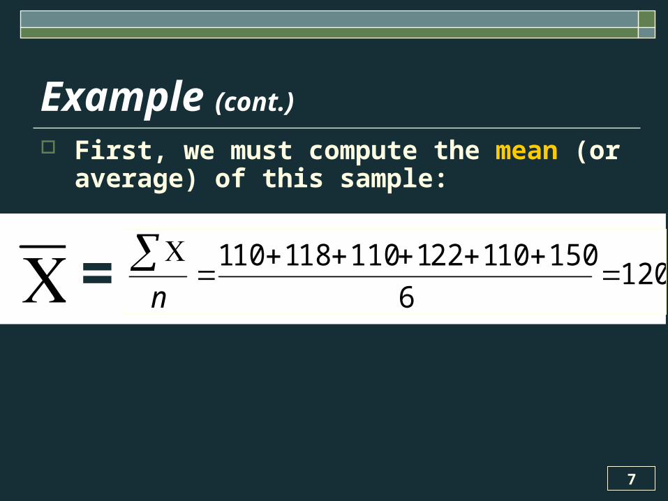
First, we must compute the mean (or average) of this sample:
1206
150101221110181101
n =

8
Example (cont.)
Notice, these 6 people have higher than
average intelligence scores (IQ 100).
1206
150101221110181101
n =

9
Example (cont.)
However, is this finding likely to hold true in repeated samples?
What if we drew 6 different people from Thorndike University?
A one-sample t-test will help answer this question.
It will tell us if our findings are ‘significant’, or in other words, likely to be repeated if we took another sample.
10
110118110122110150
120120120120120120
-10- 2-10 2-10 30
100 4100 4100900
Example (cont.)
Computing the sample variance
2)(
3.201)( 2
2
n
sx
11
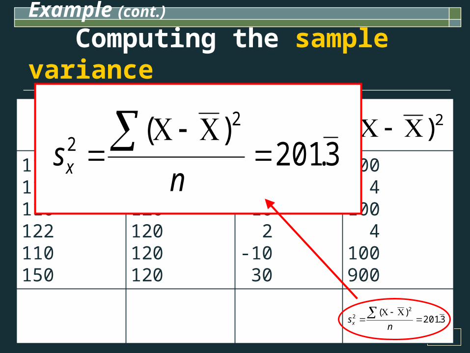
110118110122110150
120120120120120120
-10- 2-10 2-10 30
100 4100 4100900
Example (cont.)
Computing the sample variance
2)(
3.201)( 2
2
n
sx
3.201)( 2
2
n
sx
12
Example (cont.)
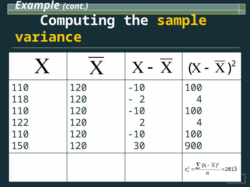
Computing the sample variance To get the third column we take each
individual ‘X’ and subtract it from the mean (120).
We square each result to get the fourth column.
Next, we simply add up the entire fourth column and divide by our original sample size (n = 6).
The resulting figure, 201.3, is the sample variance.
13
Example (cont.)
Computing the sample variance
Important: All sample variances are computed this way!
We always take the mean; subtract each score from the mean;
square the result; sum the squares;
and divide by the sample size (how many numbers, or rows we have).
14
Now that we have the mean (X = 120) and the variance ( ) of our sample, we have everything needed to compute whether the sample mean is ‘significantly’ above the average intelligence.
In the formula that follows, we use a new symbol mu ( ) to indicate the population standard value ( = 100 ) against which we compare our obtained score (X = 120).
Example (cont.)
Computing the sample variance
3.2012 xs

15
Example (cont.)
Computing the sample variance
152.3
16333.201
100120
1
2
ns
tx
Our sample has ‘n = 6’ people, so the degrees of freedom for this t-test are:
dn = n – 1 = 5This degrees of freedom figure will be used later in our test of significance.

16
And now for something completely different …
Let’s take a break from computations, and talk about ‘the big picture’
Now comes the conceptually tricky part. Remember that a normal bell-curve
distribution is a chart that shows frequencies (or counts).
If we measured the weight of four male adults, for example, we might find the following:
Person 1 = 70 kg, Person 2 = 75 kg, Person 3 = 70 kg, Person 4 = 65 kg

17
The ‘big picture’ Person 1 = 70 kg, Person 2 = 75 kg, Person
3 = 70 kg, Person 4 = 65 kg Plotting a count of these ‘weight’ data,
we find a normal distribution:
Count 2 X
1 X X X 65 70 75 kg

18
The ‘big picture’ (cont.)
As it turns out, the ‘t’ statistic has its own distribution, just like any other variable.
Let’s assume, for the moment, that the mean IQ of the population in our example is exactly 100.
If we repeatedly sampled 6 people and calculated a ‘t’ statistic each time, what would we find?
If we did this 4 times, for example, we might find:
Count 2 X
1 X X X - 1 0 1 t - statistic

19
The ‘t’ statistic (cont.)
Most often our computed ‘t’ should be around 0. Why? Because the numerator, or top part of the formula for t is: .
If our first sample of 6 people is truly representative of the population, then our sample mean should also be 100, and therefore our computed t should be (see next slide)

20
0
1
1001002
ns
tx
The ‘t’ statistic (cont.)
21
The ‘t’ statistic (cont.)
Of course, our repeated samples of 6 people will not always have
exactly the same mean as the population.
Sometimes it will be a little higher, and sometimes a little lower.
The frequency with which we find a t larger than 0 (or smaller than 0) is exactly what the t-distribution is meant to represent
(see next slide)
22
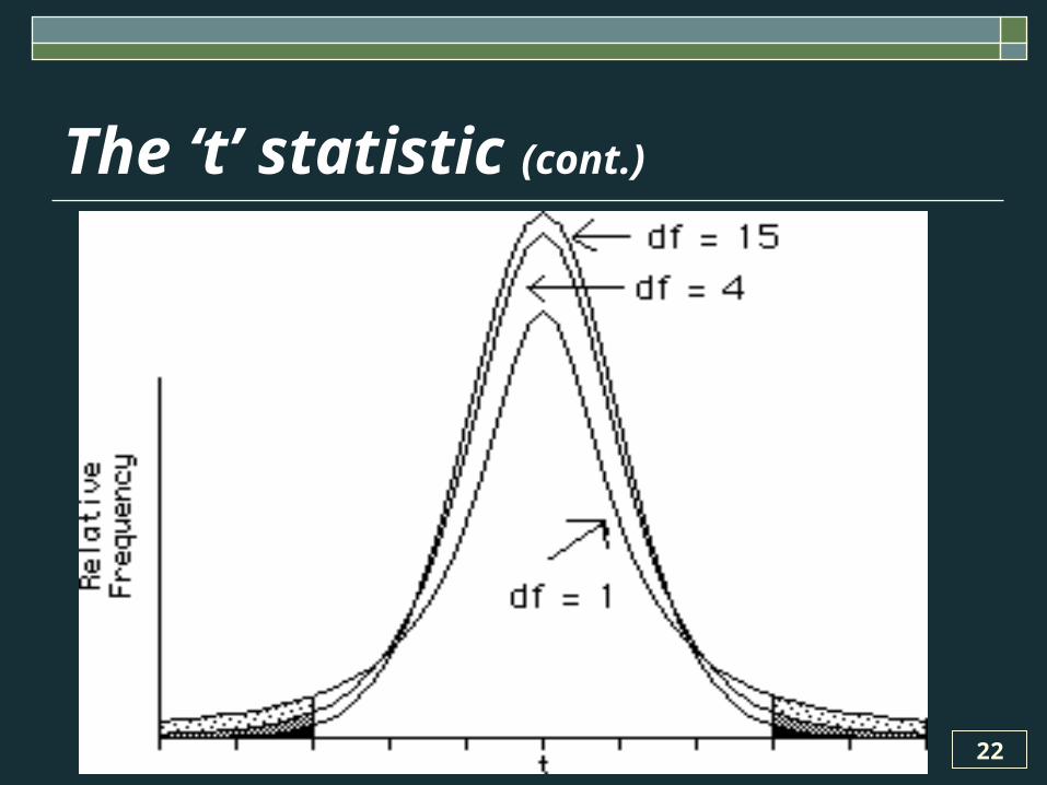
The ‘t’ statistic (cont.)

23
The ‘t’ statistic (cont.)
How do we know when our computed ‘t’ is very large in magnitude?
Fortunately, we can calculate how often a computed sample ‘t’ will be far from the population mean of t = 0 based on knowledge of the distribution.
24
The ‘t’ statistic (cont.)
The critical values of the t-distribution show exactly how often we should find computed ‘t’s of large magnitude.
In a slight wrinkle, we need the degrees of freedom (df = 5) to help us make this determination.
Why? If we sample only a few people our computed ‘t’s are more likely to be very large, only because they are less representative of the whole population.

25
And now, back to the computation… We need to find the ‘critical value’ of
our t-test. Looking in the back of any statistics
textbook, you can find a table for critical values of the t-distribution.
Next, we need to determine whether we are conducting a 1-tailed or 2-tailed t-test.
Let’s refer back to the research question:

26
Example (again)
Research Question
On average, do the population of undergraduates at Thorndike
University have higher than average intelligence scores (IQ 100)?

27
Example (cont.)
This is a 1-tailed test, because we are asking if the population mean is ‘greater’ than 100.
If we had only asked whether the intelligence of students were ‘different’ from average (either higher or lower) then the test would be 2-tailed.
In the appendixes of your textbook, look at the table titled, ‘critical values of the t-distribution’.
Under a 1-tailed test with an Alfa-level of and degrees of freedom df = 5, and you should find a critical value (C.V.) of t = 2.02.

28
Example (cont.)
Is our computed t = 3.152 greater than the C.V. = 2.02?
Yes! Thus we reject the null hypothesis
and live happily ever after.Right?
Not so fast. What does this really mean?
29
Example (still)
We assume the null hypothesis when making this test.
We assume that the population mean is 100, and therefore we will most often compute a t = 0.
Sometimes the computed ‘t’ might be a bit higher and sometimes a bit lower.

30
What does the ‘critical value’ tell us? Based on knowledge of the distribution
table we know that 95% of the time, in repeated samples, the computed ‘t’ statistics should be less than 2.02.
That’s what the critical value tells us.
It says that when we are sampling 6 persons from a population with mean intelligence scores of 100, we should rarely compute a ‘t’ higher than 2.02.

31
What happens if we do calculate a ‘t’ greater than 2.02? Well, we can be pretty confident that our
sample does not come from a population with a mean of 100!
In fact, we can conclude that the population mean intelligence must be higher than 100.
How often will we be wrong in this conclusion?
If we do these t-tests a lot, we’ll be wrong 5% of the time. That’s the Alpha level (or 5%).
32
Conclusions in APA StyleHow would we state our conclusions in APA style?
The mean intelligence score of undergraduates at Thorndike University (M = 120) was significantly higher than the standard intelligence score (M = 100), t(5) = 3.15, p < .05 (one-tailed).

33
Statistical inference You should notice that the conclusion
makes an inference about the population of students from Thorndike University based on a small sample.
This is why we call this type of a test ‘statistical inference.’
We are inferring something about the population based on only a sample of members.
34
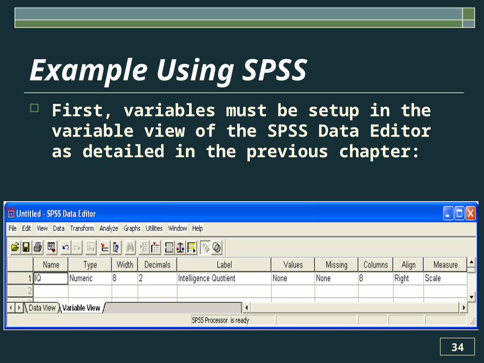
Example Using SPSS First, variables must be setup in the variable
view of the SPSS Data Editor as detailed in the previous chapter:
35
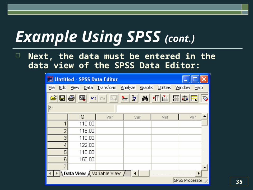
Example Using SPSS (cont.)
Next, the data must be entered in the data view of the SPSS Data Editor:
36
Instructions for the Student Version of SPSS
If you have the student version of SPSS, you must run all procedures from the pull-down menus.
Fortunately, this is easy for the one-sample t-test.
First select the correct procedure from the ‘analyze’ menu see next slide
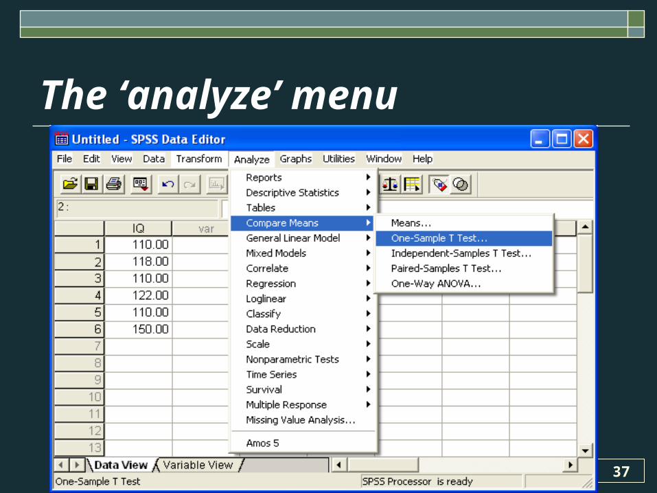
37
The ‘analyze’ menu

38
The ‘test variable’ Next, you must move the ‘test variable’, in this
case IQ, into the right-hand pane by pressing the arrow button and change the ‘test-value’ to 100 (our standard for comparison).
Lastly, click ‘OK’ to view the results:

39
Instructions for Full Version of SPSS (Syntax Method) An alternate method for obtaining the same
results is available to users of the full-version of SPSS.
This method, known as ‘syntax’, is described here, because many common and useful procedures in statistics are only available using the syntax method.
Users of the student version may wish to skip ahead to ‘Results from the SPSS Viewer.’
To use syntax, first you must open the syntax window from the ‘file’ menu:

40
The ‘file’ menu
41
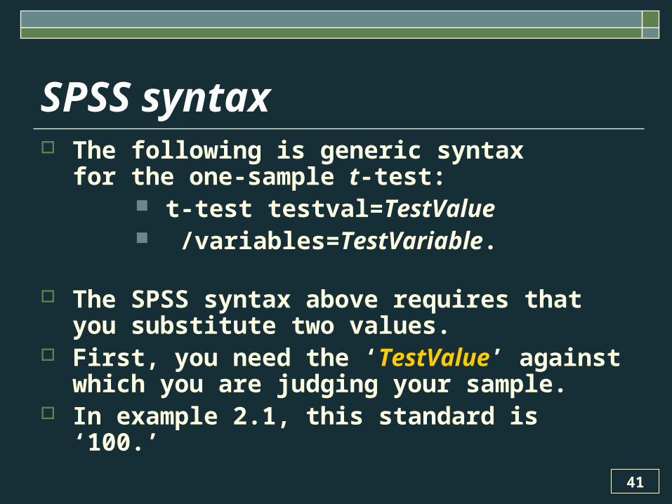
SPSS syntax The following is generic syntax
for the one-sample t-test: t-test testval=TestValue /variables=TestVariable.
The SPSS syntax above requires that you substitute two values.
First, you need the ‘TestValue’ against which you are judging your sample.
In example 2.1, this standard is ‘100.’
42
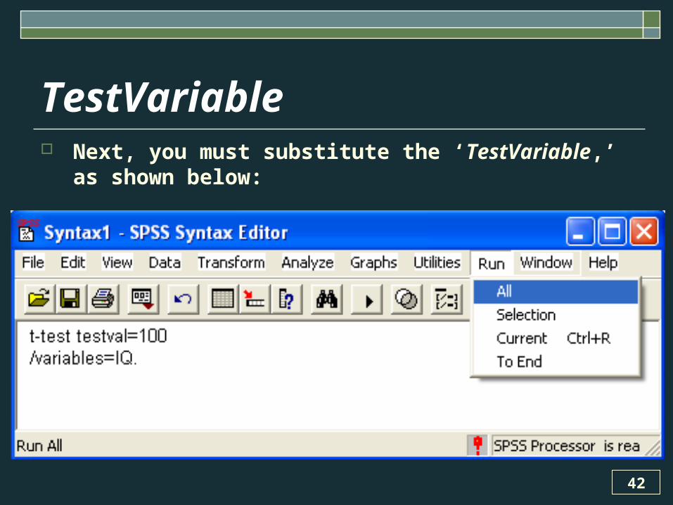
TestVariable Next, you must substitute the ‘TestVariable,’
as shown below:
43
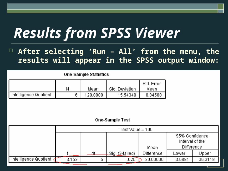
Results from SPSS Viewer After selecting ‘Run – All’ from the menu, the
results will appear in the SPSS output window:
44
SPSS calculations When using SPSS, we no longer have a
critical value to compare our calculated t-value.
Instead, SPSS calculates an exact probability value associated with the ‘t.’
As a consequence, when writing the results we simply substitute this exact value, rather than using the less precise ‘p < .05’ (per our hand-calculations above).
Notice that SPSS calls p-values ‘Sig.,’ which stands for significance.
45
SPSS calculations NOTE: SPSS only gives us the
p-value for a 2-tailed t-test.
In order to convert this value into a one-tailed test, per our example, we need to divide this ‘sig (2-tailed)’ value in half (e.g., .033/2=.02, rounded).
Why? In short, one-tailed t-tests are twice as
powerful, because we simply assume that the results cannot be different in the direction opposite to our expectations.
46
Conclusions in APA StyleFocusing attention on the bold portion of the output, we can re-write our conclusion in APA style:
The mean intelligence score of undergraduates at Thorndike University (M = 120) was significantly higher than the standard intelligence score (M = 100), t(5) = 3.15, p = .02 (one-tailed).
47
Big t Little p ? Remember from a previous session that
every t-value that we might calculate is associated with a unique p-value.
In general, t-values which are large in absolute magnitude are desirable, because they help us to demonstrate differences between our computed mean value and the standard.
Values of t that are large in absolute magnitude are always associated with small p-values.

48
Significance According to tradition in psychology,
p-values which are lower than .05 are significant, meaning that we will likely still find differences if we collected another sample of participants.
When using SPSS we are no longer confronted with a ‘critical value.’ Instead, we can simply observe that the p-value is less than ‘.05.’