1

The Luxembourg Wealth Study : enhancing comparative research on household finance

Rome, 6th July 2007

Do the elderly reduce housing equity? An international comparison

Maria Concetta Chiuri* and Tullio Jappelli**

* Università di Bari, CSEF and CHILD** Università di Napoli Federico II, CSEF and CEPR

2

Outline

Motivations

Main contribution of our paper

The evidence to date

The international dataset

Estimating ownership trajectories

Explaining international differences

in ownership trajectories

3

Motivation 1 - Policy

Population aging makes of clear policy interest understanding the determinants of decisions over:

how much to save how to save should wealth be annuitized, … etc. as people get older.

o Real estate is the largest component of total wealth (more than 70% of tot. wealth)

4

Motivation 2 - Theory Life Cycle Hypothesis (LCH) predicts

that with perfect markets selfish individuals run down their wealth in order to smooth consumption over their life-cycle

from owning to renting or downsizing.

Bequest motives Housing as a source of consumption

itself

5

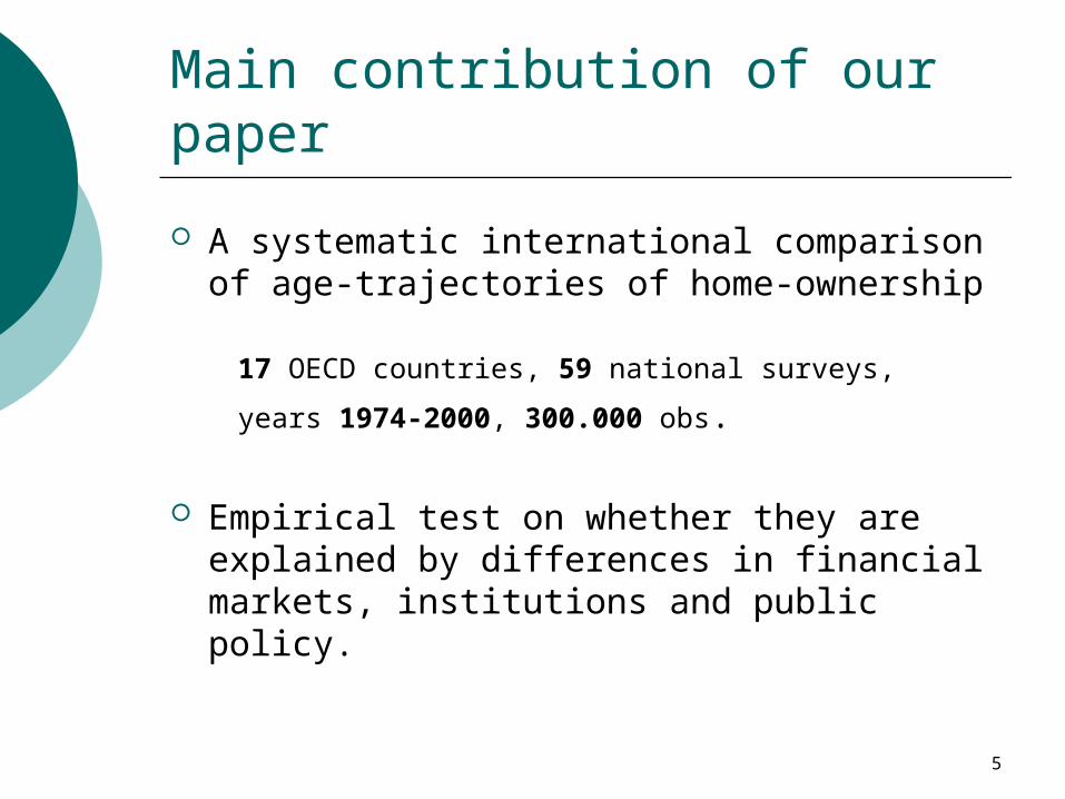
Main contribution of our paper

A systematic international comparison of age-trajectories of home-ownership

17 OECD countries, 59 national surveys,

years 1974-2000, 300.000 obs.

Empirical test on whether they are explained by differences in financial markets, institutions and public policy.

6

The evidence to date -1

US Feinstein and McFadden (1989) use PSID and find

transition from owning to renting of <0.3% per year. Venti and Wise (2002; 2004) HRRS, SIPP, AHDAOO find

1.76%; but about 8% for those with precipitating shocks; they do not depend on h/h composition. Cohort effects are relevant.

Fisher, Johnson, Marchand, Smeeding and Torrey (2007) evidence from CEX that the elderly prefer to stay in their home.

Canada Crossley and Ostrovsky (2003) use three Canadian

surveys and find an annual decline of 0.6% from age 55 to 80.

7

The evidence to date - 2

UK Ermisch and Jenkins(1999) use five waves

of BHPS and find only rare residential mobility.

Germany Börsch-Supan (1994) compare data from

Germany and the US and find that the decline is similar in the two countries.

8

Summing up – previous evidence

Decumulation, but slow

Importance of cohort effects

9

Country Survey and years available

Australia Australian Inc. and Hous. Costs Survey: 1981

Austria Micro-census: 1987, 1995; ECHP : 1997

Belgium Panel S. of CSP: 1985, 1988, 1992, 1997; Panel S. of Belgium H/h: 2000

Canada S. Consumer Fin.: 1975, 1981, 1987, 1991, 1994, 1997;

S. of Lab. and Income Dyn. 2000 Denmark Income Tax S.:1987, 1992 Finland Income Distribution S.: 1995, 2000 France Household Budget S.: 1984, 1989, 1994

Germany GSoEP : 1984, 1989, 1994, 2000 Ireland ESRI Survey: 1987; ECHP: 1994, 1996, 2000 Italy SHIW: 1986, 1991, 1993, 1995, 1998, 2000 Luxembourg Lux. Socio Econ. Panel S.: 1985, 1997, 2000

Table 1- The international dataset: the LIS project

10

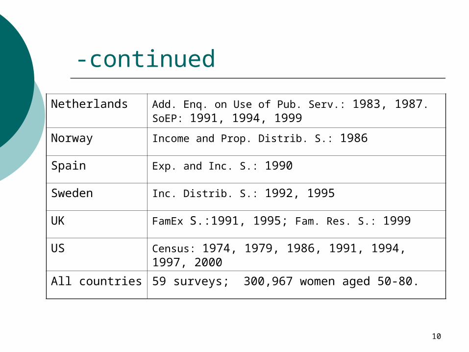
-continued

Netherlands Add. Enq. on Use of Pub. Serv.: 1983, 1987. SoEP: 1991, 1994, 1999

Norway Income and Prop. Distrib. S.: 1986

Spain Exp. and Inc. S.: 1990

Sweden Inc. Distrib. S.: 1992, 1995

UK FamEx S.:1991, 1995; Fam. Res. S.: 1999

US Census: 1974, 1979, 1986, 1991, 1994, 1997, 2000

All countries 59 surveys; 300,967 women aged 50-80.

11

Sample selection

Definition of h/h heads is biased:

Individuals rather than h/hse.g. if they move in their children’s place,

treated as renters.

Mortality rate and potential entrance in a nursing home:

women aged 50-80.

12

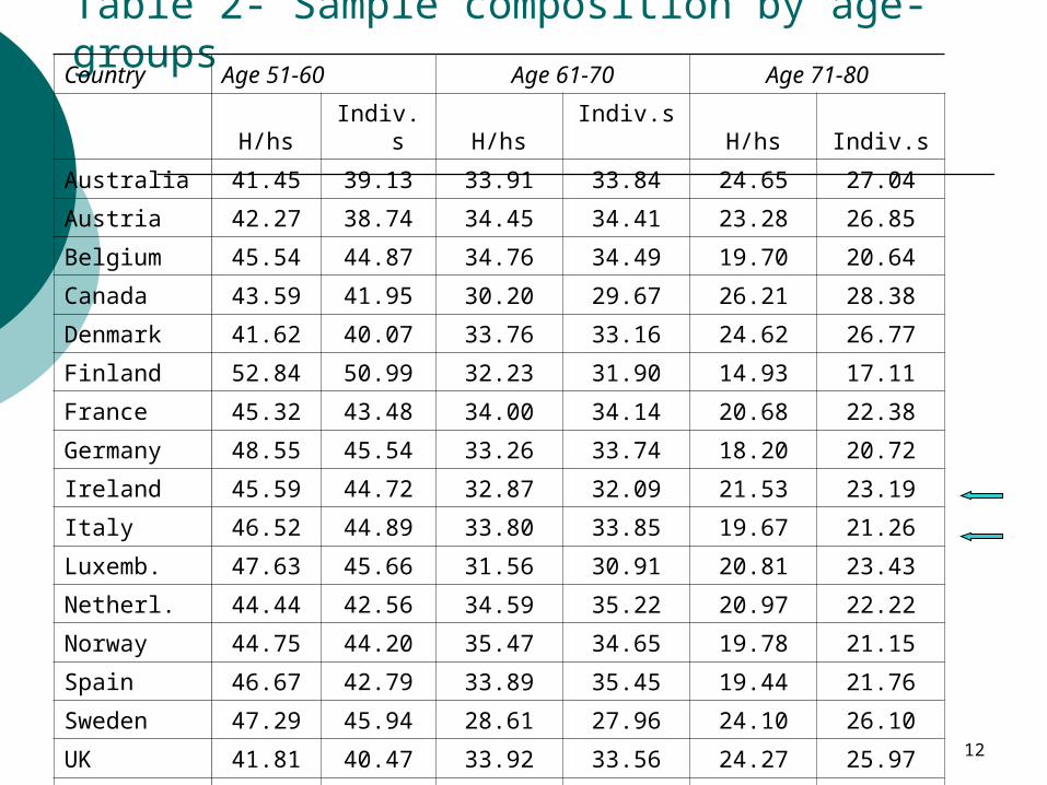
Table 2- Sample composition by age-groupsCountry Age 51-60 Age 61-70 Age 71-80

H/hs Indiv.s H/hs Indiv.s H/hs Indiv.s

Australia 41.45 39.13 33.91 33.84 24.65 27.04

Austria 42.27 38.74 34.45 34.41 23.28 26.85

Belgium 45.54 44.87 34.76 34.49 19.70 20.64

Canada 43.59 41.95 30.20 29.67 26.21 28.38

Denmark 41.62 40.07 33.76 33.16 24.62 26.77

Finland 52.84 50.99 32.23 31.90 14.93 17.11

France 45.32 43.48 34.00 34.14 20.68 22.38

Germany 48.55 45.54 33.26 33.74 18.20 20.72

Ireland 45.59 44.72 32.87 32.09 21.53 23.19

Italy 46.52 44.89 33.80 33.85 19.67 21.26

Luxemb. 47.63 45.66 31.56 30.91 20.81 23.43

Netherl. 44.44 42.56 34.59 35.22 20.97 22.22

Norway 44.75 44.20 35.47 34.65 19.78 21.15

Spain 46.67 42.79 33.89 35.45 19.44 21.76

Sweden 47.29 45.94 28.61 27.96 24.10 26.10

UK 41.81 40.47 33.92 33.56 24.27 25.97

US 46.52 44.90 31.37 31.33 22.12 23.77

13

Further data treatment

Comparability in educational attainment: ISCED classification

Survey design can vary over time

14

Table 3- Ownership by age-group (individuals)

Country Age 51-60 Age 61-70 Age 71-80

Australia 82.16 81.02 71.76

Austria 67.04 60.69 47.16

Belgium 77.60 74.89 65.33

Canada 78.62 73.73 58.98

Denmark 65.40 54.02 43.65

Finland 83.54 75.10 61.62

France 69.27 67.56 55.11

Germany 49.62 50.62 41.44

Ireland 89.93 87.82 78.24

Italy 69.74 64.36 50.02

Luxemburg 79.23 71.89 57.90

Netherlands 44.92 33.41 22.67

Norway 67.21 55.93 39.11

Spain 80.02 74.32 57.30

Sweden 75.39 69.12 53.32

United Kingdom 75.93 67.08 55.58

United States 76.52 76.92 72.03

15

Cross-sectional vs. cohort adj. profiles

In a cross-section individuals belong to different generations.

Repetead cross-sections allow to track cohorts over time.

Avg. home-ownership rates for 30 age groups (from age 51-80).

16

Estimating ownership trajectories -1

The restricted model:

[1]where:f(a) is a common third order polynomial of ageX= educ, marital and work statusb=common cohort effectγ=country fixed eff.

Model [1] is estimated with WLS using a robust Var matrix to control for neighborhood effects.

cbaccbacba bXafH ,,,,,, )(

17

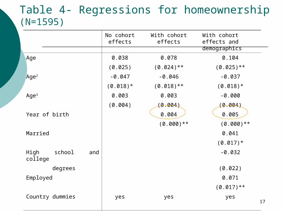
Table 4- Regressions for homeownership (N=1595)

No cohort effects

With cohort effects With cohort effects and demographics

Age 0.038 0.078 0.104

(0.025) (0.024)** (0.025)**

Age2 -0.047 -0.046 -0.037

(0.018)* (0.018)** (0.018)*

Age3 0.003 0.003 -0.000

(0.004) (0.004) (0.004)

Year of birth 0.004 0.005

(0.000)** (0.000)**

Married 0.041

(0.017)*

High school and college -0.032

degrees (0.022)

Employed 0.071

(0.017)**

Country dummies yes yes yes

R-squared 0.78 0.80 0.81

18

.4.5

.6.7

.8

50 60 70 80

Cross-sectional profile Cohort-adjusted profile

Figure 1. The cross-sectional and cohort-adjusted profile of homeownership (all countries)

19

Estimating ownership trajectories -2 The assumption that age and cohort effects are the

same in all countries is rather restrictive (an F-test rejected the null at 1 percent level).

A more general model for each single country:

[2]where:f(age) is a third-order polynomial in age. b=cohort effect

We plot the difference in cohort-adjusted ownership trajectories between 4 age groups (age 61-65, age 66-70, age 71-75 and age 76-80).

baba bagefH ,, )(

20

Figure 2. The cross-sectional and cohort-adjusted profiles of homeownership

.2.4

.6.8

1.2

.4.6

.81

.2.4

.6.8

1.2

.4.6

.81

50 60 70 80 50 60 70 80

50 60 70 80 50 60 70 80

Austria Belgium Canada Denmark

Finland France Germany Ireland

Italy Luxembourg Netherlands Sweden

UK US

Cross-sectional profile Cohort-adjusted profile

21

Figure 3. Change in ownership: from age-group 61-65 to 66-70

-.08 -.06 -.04 -.02 0 .02Change in cohort adjusted profile

US

UK

Sweden

Netherlands

Luxembourg

Italy

Ireland

Germany

France

Finland

Denmark

Canada

Belgium

Austria

22

Figure 4. Change in ownership: from age-group 66-70 to 71-75

-.08 -.06 -.04 -.02 0Change in cohort adjusted profile

US

UK

Sweden

Netherlands

Luxembourg

Italy

Ireland

Germany

France

Finland

Denmark

Canada

Belgium

Austria

23

Figure 5. Change in ownership: from age-group 71-75 to 76-80

-.08 -.06 -.04 -.02 0Change in cohort adjusted profile

US

UK

Sweden

Netherlands

Luxembourg

Italy

Ireland

Germany

France

Finland

Denmark

Canada

Belgium

Austria

24

Compare with previous findings

Negative values in all contries (after age 70)

Large differences across countries

Can we trace such differences to country characteristics?

25

Explaining international differences in ownership trajectories

o Characteristics of rental market, moving costs.

Wealth taxes, property taxes and transaction costs

The generosity of Social Security systems

o The local availability of long term care services

o Financial markets development

26

Explaining international differences in ownership trajectories

The availability of financial instruments which help house-rich but cash poor old people to release housing equity:

Reverse mortgages Mortgage equity withdrawal (trading-down,

over-mortgaging, re-mortgaging or second-mortgage)

o Regulation in financial mkt difficult to distinguish from other economy-wide regulation

27

Table 5 - Index of mortgage market and economy-wide regulation, property taxes and no. of beds in nursing homes: international comparisons

Index of mortgage market

regulation

Index of economy wide regulation

Property taxes to GDP ratio

Number of beds in nursing homes

Australia .1 .30 .027 4.8

Austria .9 .37 .006 1.7

Belgium .9 .50 .013 2.9

Canada .5 .41 .037 12.2

Denmark .3 .19 .017 5.1

Finland .5 .08 .011 4.3

France .7 .60 .024 1.3

Germany .7 .39 .01 8.6

Ireland .1 .06 .016 6.9

Italy .9 .75 .023 2.7

Luxembourg .3 .036 5.9

Netherlands .5 .08 .019 3.8

Norway .3 .34 .011 9.1

Spain .5 .42 .02 0.3

Sweden .3 .43 .02 5.4

UK .1 .0 .038 3.1

US .3 .09 .032 5.4

28

The index of mortgage market regulation is taken from Tsatsaronis and Zhu (2004). The score adds one point for fulfilling each of the following five criteria: (i) Mortgage rate arrangement are primarily extended on the basis of fixed rate contracts; (ii) Mortgage equity withdrawals is absent or limited; (iii) The loan-to-value ratio does not exceed 75 percent, (iv) Valuation methods of property is based on historical values, rather than based on market values (v) Mortgage backed securitization is absent or limited. The index is then normalized to one.

The index of economy wide regulation is taken from Kaufman, Kraay and Zoldo Lobaton (1999). The index is a very wide indicator of the degree of economic regulation covering many different regulatory areas (state control, barriers to entrepreneurship, administrative regulations, tariff and non-tariff barriers, etc.) aggregated through factor analysis.

29

Figure 6. Change in ownership and mortgage market regulation

Ireland

UK

Denmark

Luxembourg

USSweden

Finland

Netherlands

Canada

France

Germany

Belgium

Austria

Italy

-.1

-.0

8-.

06

-.0

4-.

02

0

0 .1 .2 .3 .4 .5 .6 .7 .8 .9 1

Ch

ange

in o

wn

ersh

ip

Index of mortgage market regulation

Note. Cohort-adjusted change in ownership between age 71-75 and age 76-80.

30

Figure 7. Change in ownership and economy-wide regulation

Note. Cohort-adjusted change in ownership between age 71-75 and age 76-80.

UK

Ireland

Netherlands

Finland

USDenmark

Austria

Germany

Canada

Sweden

Belgium France

Italy

-.1

-.0

8-.

06

-.0

4-.

02

0

0 .1 .2 .3 .4 .5 .6 .7 .8

Ch

ange

in o

wn

ersh

ip

Index of economy-wide regulation

31

Table 6 Regressions for change in ownership

(1) (2) (3) (4) (5) (6)

Index of mortgage -0.045 -0.048

market regulation (0.018)** (0.024)*

Index of economy- -0.063 -0.060

wide regulation (0.016)*** (0.016)***

Property tax to GDP 1.006 0.096 0.187

ratio (0.730) (0.641) (0.416)

Number of beds in 0.003 -0.001 -0.001

nursing homes (0.003) (0.003) (0.002)

Ownership in age -0.020 -0.011 -0.036 -0.007 -0.029 -0.019

group 71-75 (0.036) (0.028) (0.054) (0.050) (0.035) (0.026)

Constant 0.003 -0.008 -0.032 -0.042 0.016 -0.003

(0.030) (0.020) (0.039) (0.042) (0.041) (0.024)

Observations 14 13 14 13 13 12

R-squared 0.36 0.61 0.15 0.06 0.49 0.72

32

Sensitivity analysis

Lagged ownership

Overall ownership rate (proxy for thin rental mkt)

Property vs. transaction taxes

Social security income replacement rate

Price to income ratio

33

Conclusion We estimated the home-ownership rate for the

elderly using data from 17 OECD countries.

The analysis at the individual level

Controlling for cohort effects, the ownership rate falls after age 70; after age 75 falls at 1% per year.

Differences across countries are highly explained by the degree of morgage mkt regulation and by the economy-wide regulation.

Credit market imperfections are an explanatory factor for international differences in the aggregate saving rate.