1

The General 2k Factorial Design

• Section 6-4, pg. 224, Table 6-9, pg. 225

• There will be k main effects, and

two-factor interactions2

three-factor interactions3

1 factor interaction

k

k

k

2

General Procedure for a 2k Factorial Design

• Estimate factor effects (sign & magnitude)

• From initial model (usually the full model)

• Perform statistical testing (ANOVA)

• Refine model (removing nonsignificant variables)

• Analyze residuals (model adequacy/assumptions checking)

• Refine model if it’s necessary• Interpret results (main/interaction effects plots,

contour plots, response surfaces)

3

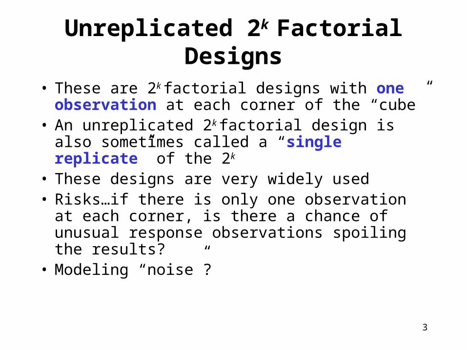
Unreplicated 2k Factorial Designs

• These are 2k factorial designs with one observation at each corner of the “cube”

• An unreplicated 2k factorial design is also sometimes called a “single replicate” of the 2k

• These designs are very widely used• Risks…if there is only one observation at each

corner, is there a chance of unusual response observations spoiling the results?

• Modeling “noise”?

4

Spacing of Factor Levels in the Unreplicated 2k

Factorial Designs

If the factors are spaced too closely, it increases the chances that the noise will overwhelm the signal in the data

More aggressive spacing is usually better

5

Unreplicated 2k Factorial Designs

• Lack of replication causes potential problems in statistical testing– Replication admits an estimate of “pure error” (a better

phrase is an internal estimate of error)– With no replication, fitting the full model results in

zero degrees of freedom for error

• Potential solutions to this problem– Pooling high-order interactions to estimate error– Normal probability plotting of effects (Daniels, 1959)– Other methods…see text, pp. 234

6

Example of an Unreplicated 2k Design

• A 24 factorial was used to investigate the effects of four factors on the filtration rate of a resin

• The factors are A = temperature, B = pressure, C = mole ratio/concentration, D= stirring rate

• Experiment was performed in a pilot plant

7

The Resin Plant Experiment

8

The Resin Plant Experiment

9

Estimates of the Effects

Term Effect SumSqr % Contribution

Model Intercept

Error A 21.625 1870.56 32.6397Error B 3.125 39.0625 0.681608Error C 9.875 390.062 6.80626Error D 14.625 855.563 14.9288Error AB 0.125 0.0625 0.00109057Error AC -18.125 1314.06 22.9293Error AD 16.625 1105.56 19.2911Error BC 2.375 22.5625 0.393696Error BD -0.375 0.5625 0.00981515Error CD -1.125 5.0625 0.0883363Error ABC 1.875 14.0625 0.245379Error ABD 4.125 68.0625 1.18763Error ACD -1.625 10.5625 0.184307Error BCD -2.625 27.5625 0.480942Error ABCD 1.375 7.5625 0.131959

10

The Normal Probability Plot of EffectsDESIGN-EXPERT PlotFiltration Rate

A: TemperatureB: PressureC: ConcentrationD: Stirring Rate

Normal plot

No

rma

l % p

rob

ab

ility

Effect

-18.12 -8.19 1.75 11.69 21.62

1

5

10

20

30

50

70

80

90

95

99

A

CD

AC

AD

11

The Half-Normal Probability Plot DESIGN-EXPERT PlotFiltration Rate

A: TemperatureB: PressureC: ConcentrationD: Stirring Rate

Half Normal plot

Ha

lf N

orm

al %

pro

ba

bili

ty

|Effect|

0.00 5.41 10.81 16.22 21.63

0

20

40

60

70

80

85

90

95

97

99

A

CD

AC

AD

12

ANOVA Summary for the Model

Response:Filtration Rate ANOVA for Selected Factorial ModelAnalysis of variance table [Partial sum of squares]

Sum of Mean FSource Squares DF Square Value Prob >FModel 5535.81 5 1107.16 56.74 < 0.0001A 1870.56 1 1870.56 95.86 < 0.0001C 390.06 1 390.06 19.99 0.0012D 855.56 1 855.56 43.85 < 0.0001AC 1314.06 1 1314.06 67.34 < 0.0001AD 1105.56 1 1105.56 56.66 < 0.0001Residual 195.12 10 19.51Cor Total 5730.94 15

Std. Dev. 4.42 R-Squared 0.9660Mean 70.06 Adj R-Squared 0.9489C.V. 6.30 Pred R-Squared 0.9128

PRESS 499.52 Adeq Precision 20.841

13

The Regression Model

Final Equation in Terms of Coded Factors:

Filtration Rate =+70.06250+10.81250 * Temperature+4.93750 * Concentration+7.31250 * Stirring Rate-9.06250 * Temperature * Concentration+8.31250 * Temperature * Stirring Rate

14

Model Residuals are SatisfactoryDESIGN-EXPERT PlotFiltration Rate

Studentized Residuals

No

rma

l % p

rob

ab

ility

Normal plot of residuals

-1.83 -0.96 -0.09 0.78 1.65

1

5

10

20

30

50

70

80

90

95

99

15

Model Interpretation – InteractionsDESIGN-EXPERT Plot

Filtration Rate

X = A: TemperatureY = C: Concentration

C- -1.000C+ 1.000

Actual FactorsB: Pressure = 0.00D: Stirring Rate = 0.00

C: ConcentrationInteraction Graph

Filt

ratio

n R

ate

A: Temperature

-1.00 -0.50 0.00 0.50 1.00

41.7702

57.3277

72.8851

88.4426

104

DESIGN-EXPERT Plot

Filtration Rate

X = A: TemperatureY = D: Stirring Rate

D- -1.000D+ 1.000

Actual FactorsB: Pressure = 0.00C: Concentration = 0.00

D: Stirring RateInteraction Graph

Filt

ratio

n R

ate

A: Temperature

-1.00 -0.50 0.00 0.50 1.00

43

58.25

73.5

88.75

104

16

Model Interpretation – Cube PlotDESIGN-EXPERT Plot

Filtration RateX = A: TemperatureY = C: ConcentrationZ = D: Stirring Rate

Actual FactorB: Pressure = 0.00

Cube GraphFiltration Rate

A: Temperature

C: C

on

cen

tra

tion

D: Stirring Rate

A- A+C-

C+

D-

D+

46.25

44.25

74.25

72.25

69.38

100.63

61.13

92.38

If one factor is dropped, the unreplicated 24 design will project into two replicates of a 23

A unreplicated 2k design, if h (h<k) factors are negligible, then the original data -> a full two-level factorial 2k-h with 2h replicates.

Design projection is an extremely useful property, carrying over into fractional factorials

17

The Resin Plant Experiment

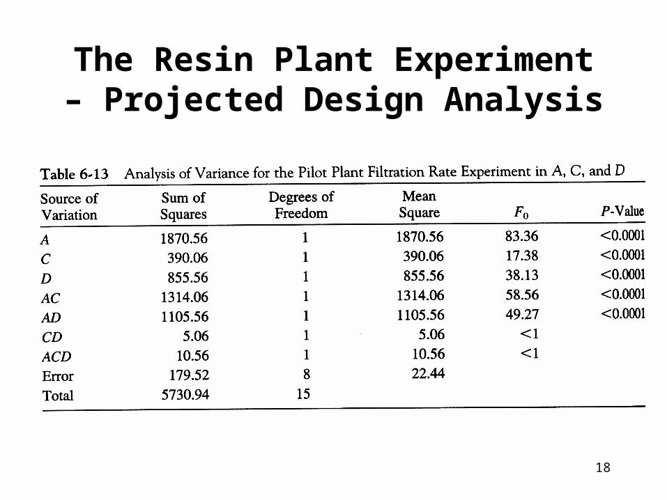
18

The Resin Plant Experiment – Projected Design Analysis

19

Model Interpretation – Response Surface Plots

DESIGN-EXPERT Plot

Filtration RateX = A: TemperatureY = D: Stirring Rate

Actual FactorsB: Pressure = 0.00C: Concentration = -1.00

44.25

58.3438

72.4375

86.5313

100.625

F

iltr

ati

on

Ra

te

-1.00

-0.50

0.00

0.50

1.00

-1.00

-0.50

0.00

0.50

1.00

A: Temperature D: Stirring Rate

DESIGN-EXPERT Plot

Filtration RateX = A: TemperatureY = D: Stirring Rate

Actual FactorsB: Pressure = 0.00C: Concentration = -1.00

Filtration Rate

A: Temperature

D: S

tirri

ng

Ra

te

-1.00 -0.50 0.00 0.50 1.00

-1.00

-0.50

0.00

0.50

1.00

64.62571

77.375

83.75

90.125

56.93551.9395

With concentration at either the low or high level, high temperature and high stirring rate results in high filtration rates