1 Spark Ignition Engine Fuel-to-Air Ratio Control: An Adaptive Control Approachweb.mit.edu/aaclab/pdfs/far_012209_delete.pdf · 2009-01-24 · 1 Spark Ignition Engine Fuel-to-Air

1

Spark Ignition Engine Fuel-to-Air Ratio

Control: An Adaptive Control Approach

Yildiray Yildiz, Student Member, IEEE, Anuradha M. Annaswamy, Fellow, IEEE,

Diana Yanakiev, Member, IEEE, Ilya Kolmanovsky, Fellow, IEEE

Abstract

This paper presents the control of Spark Ignition (SI) Internal Combustion (IC) engine Fuel-to-Air

Ratio (FAR) using an adaptive control method of time-delay systems. The objective is to maintain the

in-cylinder FAR at a prescribed set point, determined primarily by the state of the Three-Way Catalyst

(TWC), so that the pollutants in the exhaust are removed with the highest efficiency. The FAR controller

must also reject disturbances due to canister vapor purge and inaccuracies in air charge estimation and

wall-wetting (WW) compensation. Two adaptive controller designs are considered. The first design is

based on feedforward adaptation while the second design is based on both feedback and feedforward

adaptation incorporating the recently developed Adaptive Posicast Controller (APC). We present both

simulation and experimental results demonstrating the performance improvement by employing the APC.

We also present the modifications and improvements to the APC structure which were developed during

the course of experimentation to solve specific implementation problems.

Index Terms

Road vehicles, internal combustion engines, adaptive control, delay effects

I. INTRODUCTION

Triggered by the governmental regulations on emissions in 1960’s and 1970’s, the introduction

of the microprocessor based control permitted the automotive manufacturers to design cleaner,

Y. Yildiz and A. M. Annaswamy are with the Department of Mechanical Engineering, Massachusetts Institute of Technology,

Cambridge, MA, 02139 USA (e-mail: [email protected], [email protected]).

Diana Yanakiev and Ilya Kolmanovsky are with the Research and Innovation Center, Ford Motor Company, Dearborn, MI,

48121 USA (email: [email protected], [email protected]).

Manuscript received November ??, 2008; revised January ??, 2009.

January 22, 2009 DRAFT

2

more fuel efficient, better performing and more reliable powertrain systems. The associated

control problems provide continuing challenges to control engineers as the requirements pro-

gressively become more stringent. Higher levels of performance and robustness are expected,

while the calibration time and effort need to be reduced. Advances in control theory can be

exploited to address these challenges. See [1] for an introduction to modeling and control of

internal combustion engines.

The Fuel-to-Air Ratio (FAR) control is one of the most important control problems for

conventional gasoline engines. The FAR control performance can strongly impact key vehicle

attributes such as emissions, fuel economy and drivability. For instance, the FAR in engine

cylinders must be controlled in such a way that the resulting exhaust gases can be efficiently

converted by the Three-Way Catalyst (TWC). The TWC efficiency is about 98 percent when the

fuel is matched to air charge in stoichiometric proportion and drops abruptly outside a narrow

region as seen in Fig. 1 [2]. The TWC can also compensate for the temporary FAR deviation

from stoichiometry, by either storing excess oxygen or releasing oxygen to convert excess hydro-

carbons (HC) and carbon monoxide (CO). Thus, for the TWC to operate efficiently, the stored

oxygen level must be regulated so that a range to accommodate further release or storage during

transient conditions is available [1]. The oxygen storage level in the TWC may be inferred on

the basis of the TWC model and a signal from a switching Heated Exhaust Gas Oxygen (HEGO)

sensor located downstream of the TWC. In addition, the oxygen storage capacity of the TWC

depends on the size and precious metal loading of the TWC. Therefore, if the FAR excursions

and their durations are reduced with a well-performing controller, the storage capacity of TWC

and its cost may be reduced as well.

A conventional FAR control system includes two nested controllers. The outer-loop controller

generates a reference FAR (set-point) for the inner-loop controller based, for instance, on the

deviation of the estimated TWC stored oxygen state. The inner-loop controller maintains the

FAR upstream of the TWC at this set-point by using the measurements of the feedgas FAR with

a linear Universal Exhaust Gas Oxygen (UEGO) sensor to appropriately correct engine fueling

rate. Small amplitude low frequency periodic modulation may be superimposed over the set-

point to further improve catalyst efficiency. The HEGO sensor downstream of the TWC is also

used to improve robustness to UEGO sensor drifts, changes to fuel type, and for diagnostics.

The inner loop controller consists of a feedforward component which is fast but may not


3

Fig. 1. TWC efficiency vs. air-to-fuel ratio.

be always accurate, and a feedback component which is slower but eliminates the steady-state

error [1]. The feedforward component consists of estimation of the air and fuel path dynamics

combined with appropriate compensations. These air and fuel dynamics correspond, mainly, to

the intake manifold lag that affects the air charge, and the wall-wetting (WW) that determines the

amount of fuel inducted into the cylinder for each fuel injection event during transient operation.

The FAR control problem has been extensively investigated over many years. In terms of

advanced approaches, here we mention the use of nonlinear feedforward controllers [3], adaptive

controllers [4], [5], [6], [7], feedback linearization [8], observer based controllers [9], [10], [11],

sliding mode controllers [12], [13], [14], linear quadratic regulators [15], [16], H8 controllers

[17], [18], Smith Predictors [19], neural network controllers [20] and model predictive controllers

[21]. The use of an electronic throttle as an additional control actuator [22] or secondary/port

throttles [23] has been also explored. Apart from stoichiometric FAR controllers, reference [24]

considers control of FAR in a lean burn engine using linear parameter-varying controllers. In

addition to these control research, [25] presents an interesting example of estimating the FAR in

the cylinders without using the oxygen sensor and thus reducing the time delay in the system,


4

and [26] presents a research result on estimating the fuel-film dynamics. The motivation for

these and related studies has been to achieve improved performance and robustness of the FAR

control thereby enabling emission, fuel economy and drivability improvements.

Main challenges in the design of the FAR controller include variable time delay, uncertain

plant behavior and disturbances. The time delay in the system comprises two basic components

[24]: the time it takes from the fuel injection calculation to exhaust gas exiting the cylinders and

the time it takes for the exhaust gases to reach the UEGO sensor location. The time delay in the

system is a key factor limiting the bandwidth of the FAR feedback loop. The plant uncertainties

are the result of inaccuracies in the air charge estimation and in the WW compensation, as well

as changes in the UEGO sensor due to aging. When the carbon canister, which stores the fuel

vapor generated in the fuel tank, is purged, the fuel content in the purge flow into the intake

manifold is also uncertain and creates disturbance to the FAR control loop.

We, therefore, are interested in a control approach which can handle both uncertainties and

large time-delays, and that can achieve a high performance. Literature, given above, about

classical and advanced control applications to the FAR control problem proves the success of an

automatic, model based control approach, and our work built upon these results by eliminating the

need of a precise engine model for classical or optimization based algorithms and by eliminating

the conservatism introduced by the robust control approaches. This is achieved by using the

Adaptive Posicast Controller (APC) [27], [28], which is an adaptive controller for time delay

systems. Successful adaptive control approaches are presented also in references [4], [5], [6]

and [7], but our approach is different from them: In [4] and [6], a nonlinear least squares

parameter identification method is used to identify the plant parameter values online and then

use these values in the controller. For the convergence of these parameters, the condition of

persistent excitation is needed. In addition, this online parameter identification may require extra

computational power. In both of the references, the controllers are applied to a single cylinder

laboratory engine. In [5], again a similar approach is taken where an extended Kalman Filter is

used to identify the plant parameter values online. Similarly, in [7], the authors use a step by

step experimental procedure to identify the sensor time constant, during the time of operation,

where a rich input excitation is needed for parameter convergence. Our approach is based on

direct adaptation where an online parameter identification scheme is not used. In addition, we

apply the APC to a Lincoln Navigator test vehicle with 8 cylinders, which makes the control


5

task much harder due to cylinder to cylinder variations. Finally, in our work, we do not only

present our results but also give a comparison with the existing control design in the test vehicle

and with a gain scheduled Smith Predictor.

The Adaptive Posicast Control (APC) is a recently developed control design approach that

is especially suited for plants with large time-delays [27], [28] and parametric uncertainties.

The APC can be described as an adaptive controller that combines explicit delay compensation,

using the classical Smith Predictor [29] and finite spectrum assignment [30], and adaptation [31],

[32]. Due to such a unique combination, the APC effectively deals with both uncertainties and

large time-delays both of which are dominant features of the FAR control problem. Previously,

the authors explained preliminary implementation results of this controller to idle speed control

and FAR control problems in conference papers [33], [34] and [35]. This paper expands on

those results with further theoretical improvements, new experimental results and more detailed

explanations of the experimental issues.

To fit the specific needs of the FAR application, our design has been extended with additional

features: First, an adaptive feedforward term is added which is crucial for disturbance rejection.

Second, procedures are developed for the controller parameter initialization and the adaptation

rate selection to reduce the calibration time and effort. Third, an algorithm to take care of the

variable delay is introduced. Fourth, an anti-windup logic is used to prevent the winding up the

integrators used for parameter adaptation. Finally, a robustifying scheme is used to prevent the

drift of the adaptive parameters. Our main contribution is the demonstration of the potential of

this adaptive controller to improve the performance and to reduce the time and effort required

for the controller calibration. This is achieved by the help of modifications and improvements

that are listed above.

The experimental results obtained using a Lincoln Navigator test vehicle provided by Ford

Motor Company, Dearborn, USA, demonstrate the capability of the controller to improve per-

formance and decrease the calibration time and effort.

Adaptive Posicast FAR control approach represents a step towards a fully self-calibrating FAR

controller because it reduces reliance on feedforward characterization and because the controller

gains are automatically tuned online.

For comparison with the APC, we also develop in this paper a feedforward adaptive controller

that attempts to minimize the impact of the purge fuel disturbance. We also compare this


6

controller with the baseline controller using simulations and in-vehicle experiments.

While our control approach is adaptive, its development both benefits from and depends on

the structural properties of the underlying plant model. This plant model for FAR ratio control

is briefly discussed next, while the reader is referred to [1] for a more extended treatment of the

underlying modeling techniques.

II. PLANT MODEL

A block diagram representation of the plant, from fuel injection to the universal exhaust

gas oxygen (UEGO) sensor measurement, together with the TWC is shown in Fig. 2, where

“A” stands for the air charge that is calculated based on the driver torque command. The fuel

inducted into the engine cylinders is viewed as the sum of the output the WW dynamics block

and the canister purge, while the fuel injected by the injectors is an input to the WW block.

The multiplication by the gain in the “1A” block gives the FAR of the mixture in the engine

cylinders (we will consider the control of FAR as opposed to air-to-fuel ratio (AFR) since it

scales linearly with fuel) and the delay block represents the combined effect of time delays in

the system. The largest contributors to that delay are the time from the fuel injection to exhaust

gas formation and the time needed for the exhaust gases to reach the UEGO sensor location.

Finally, the exhaust gases undergo mixing, FAR is measured by the UEGO sensor and then the

mixture passes through the TWC to get stripped from its pollutants.

In the model we use, the input is the mass flow rate of fuel injected by the injectors and the

output is the equivalence ratio, which is the fuel to air ratio normalized by its stoichiometric

value, measured by the UEGO sensor in the exhaust. As explained above, there are mainly four

components of the FAR dynamics which are wall-wetting dynamics, fuel-air mixture formation,

mixture propagation to the UEGO sensor location and finally UEGO sensor dynamics. Below,

the modeling aspects for each component together with their transfer functions are explained.

A. Wall-Wetting (WW) Dynamics

After the fuel is injected by the injectors, some of the fuel immediately evaporates and is

inducted into the engine cylinders, while the rest replenishes a liquid fuel puddle, which forms

on the walls of the intake ports and on the intake valves. A fraction of the fuel evaporates


7

Canister

Purge

Wall

WettingΣΣΣΣ 1/ A

Gas

mixingDelay UEGO TWC

Driver

Command

Injected

Fuel

FAR

measured

Fig. 2. Plant block diagram representation.

from the liquid puddle and is also inducted into the engine cylinders. A WW dynamics model

represents this phenomenon with the following transfer function.

Fcpsq

Fipsq

1 p1 Xqτvs

τvpsq 1(1)

where Fc, Fi, X and τv represent the fuel entering the cylinders, injected fuel, the fraction of

the fuel contributing to the fuel puddle and the puddle evaporation time constant, respectively.

B. FAR Formation and Propagation to the UEGO Sensor

The vaporized fuel mixes with the air and forms the fuel-air mixture. This process may be

modeled as a division of the fuel mass by the air mass, Aptq, entering the cylinder. Starting

from the opening of the intake valve, it takes approximately one engine cycle, i.e., 2 crankshaft

revolutions, until the exhaust gases fully exit the cylinder. This delay is called the cycle delay, τc,

and can be approximated as τc 120N , where N is the engine speed in revolutions-per-minute.

After the exhaust gases exit the cylinder, they mix with the previously existing exhaust gases

and travel through the exhaust manifold until they reach the UEGO sensor location. Also, in a

multi-cylinder engine, the exhaust gases coming from the individual cylinders enter the exhaust

manifold at different times. All these effects can be modeled by a pure delay element in series

with a first order lag asΦbmpsq

Φengpsq

1

τgmpsq 1eτtr (2)

where, Φbm, Φeng, τgm and τtr represent the equivalence ratio, which is fuel-to-air ratio divided

by stoichiometric (desired) fuel-to-air ratio, just before the measurement, equivalence ratio right

after the engine exit, gas mixing time constant and transport delay, respectively.


8

C. Sensor Dynamics

Sensor dynamics can be modeled by a first order lag as

Φmpsq

Φbmpsq

1

τspsq 1(3)

where Φmpsq and τs represent the measured equivalence ratio and sensor time constant, respec-

tively.

D. Reduced Order Model

When all the individual elements of FAR dynamics described in eqns. (1)-(3) are combined,

a third order transfer function in series with a pure delay is obtained. To simplify the controller

design, a first order lag in series with a pure time delay is used as a reduced order plant model,

where the input and the output are the deviations in the commanded in-cylinder equivalence

ratio and the measured equivalence ratio.

Gpsq 1

τms 1eτs (4)

Accurate WW compensation (effectively, the feedforward inversion of (1)) helps to render this

approximation more valid. Using relay feedback identification method for time delay systems

[36] the coefficients of this model at around the speed of 700 rpm and in warm conditions are

found to be 0.4 and 0.45 for τm and τ , respectively. Note that τ consists of the cycle delay

τc and the transport delay τtr and it also accounts for the UEGO sensor time delay and the

computational delay in the engine control unit.

III. CONTROLLER DESIGN

The structure of the closed loop system used in the test vehicle is presented in Fig. 3. The

figure shows the inner and the outer control loops. The outer loop determines the desired FAR,

pF Aqd, depending on the state of the TWC, measured by the HEGO sensor. pF Aqd becomes

the reference for the inner loop controller or the feedback controller, which is referred to as

“Controller”. The air estimate, referred to as A, depends on the driver torque request. The

multiplication of pF Aqd with A is referred to as the “base fuel”, Fb, which is an estimate

of the desired fuel. The feedback controller corrects this estimate using the UEGO sensor

measurement of the FAR upstream of the TWC. Note that the feedback controller applies a


9

Reference

Generator

Canister

Purge

Wall


Gas

MixingDelay UEGO TWCA

Driver

Command

ΣΣΣΣController

X

dA

F

mA

F

dA

F

HEGO

Wall W

Compb

F

u

cu

Fig. 3. Overall closed loop controller structure.

multiplicative correction as opposed to additive correction, although the latter is more typical in

controls literature. The advantage of the multiplicative feedback over additive feedback is that

the feedback fuel quantity scales proportionally to the value of the base fuel thereby providing

better ability to compensate in transients when changes in vehicle operating point occur as

this multiplicative transformation maintains the dc gain of the Plant assumed for fuel-to-air ratio

feedback design constant across the vehicle operating range. In addition to the feedback controller

there is a WW compensation algorithm in the system which estimates the WW dynamics and

use the inverse dynamics to cancel it.

What we are interested in is the feedback controller, for which we design two different adaptive

controllers with different complexity. Before explaining these designs, we explain the baseline

controller first, which is the existing feedback controller in the vehicle.

A. Baseline Controller

The baseline controller in the vehicle is essentially a gain-scheduled Proportional-plus-Integral

(PI) controller. In the actual vehicle implementation, a first-order filter in series with PI controller

and relay logic are used. Note that before the feedback control input is multiplied by the base

fuel Fb, it is shifted by 1. So the resulting control input for the baseline controller can be given


10

as

uc p1 uqFb, (5)

where uc is the total control signal without the WW compensation and u is the output of the

feedback controller. This structure has the advantage of a feedback control input u that has

relatively small values, since it’s bias, 1, is already causing the control signal uc to be equal to

the required base fuel Fb.

Note that, to maintain stability in the presence of delay, the gains of the PI controller cannot

be made very aggressive. Moreover, due to the delay in the system, the overshoot in the response

is difficult to avoid using this feedforward-feedback combination.

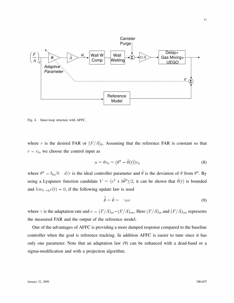
B. Adaptive Feedforward Controller (AFFC)

The system diagram with the Adaptive Feedforward Controller (AFFC) is shown in Fig. 4.

This is a simple model reference adaptive controller, where it is assumed that the only uncertainty

occurs in the control input gain. Instead of the feedback path in Fig. 3, a gain multiplier on

the pF Aqd is adapted. Note that the outer loop is not shown in the figure. The motivation

for AFFC is to compensate for errors in the base fuel calculation due to, for example, injector

uncertainties or “lost-fuel” effects present at cold engine conditions. Assuming that the desired

FAR is in general constant and equal to stoichiometric FAR, it can be shown that this controller

can also reject constant disturbances.

To derive the adaptation law, consider the following reduced order plant model represented in

state space form with a constant disturbance

9xp axp bpupt τq dq (6)

where, xp represents the measured FAR, a and b are known and unknown constants respectively

and d is a constant, unknown disturbance. Since the plant is stable, a is negative and since b

represents the gain of the injectors, it is positive. Note that since reduced order dynamics is first

order, (6) is a scalar differential equation.

Consider a reference model

9xm axm bmrpt τq (7)


11

Canister

Purge

Wall


Delay+

Gas Mixing+

UEGOA

dA

F

Wall W

Compc

uθ

Reference

Model

ΣΣΣΣe

Adaptive

Parameter

Fig. 4. Inner-loop structure with AFFC.

where r is the desired FAR or pF Aqd. Assuming that the reference FAR is constant so that

r r0, we choose the control input as

u θr0 pθ θptqqr0 (8)

where θ bmb dr is the ideal controller parameter and θ is the deviation of θ from θ. By

using a Lyapunov function candidate V pe2 bθ2q2, it can be shown that θptq is bounded

and limtÑ8eptq 0, if the following update law is used

9θ 9θ γer (9)

where γ is the adaptation rate and e pF AqmpF Aqrm. Here pF Aqm and pF Aqrm represents

the measured FAR and the output of the reference model.

One of the advantages of AFFC is providing a more damped response compared to the baseline

controller when the goal is reference tracking. In addition AFFC is easier to tune since it has

only one parameter. Note that an adaptation law (9) can be enhanced with a dead-band or a

sigma-modification and with a projection algorithm.


12

C. Adaptive Posicast Controller (APC)

As discussed above, AFFC can handle the uncertainties in the controller gain. However, in

reality there are more uncertainties in the system resulting from, for example, the actuator aging

or simply from the operating point changes such as varying temperatures, speeds and loads. All

these effects can change the system dominant pole. Therefore, we need a controller that can also

adapt to these uncertainties, and that makes the APC a good candidate.

APC is a model reference adaptive controller for systems with known input delay. Below,

we summarize the main idea behind the APC. The the reader is referred to [28] for additional

details. Consider a linearized plant with input-output description given as

yptq Wppsqupt τq, Wppsq kpZppsq

Rppsq(10)

where y is the measured plant output, u is the control input, and Wppsq is the delay-free part of

the plant transfer function. Rppsq is the nth order denominator polynomial, not necessarily stable

and the numerator polynomial, Zppsq has only minimum phase zeros. The relative degree, n,

which is equal to the order of the denominator minus the order of the numerator, is assumed to

be smaller or equal to two. It is also assumed that the delay and the sign of the high frequency

gain kp are known, but otherwise Wppsq may be unknown. Suppose that the reference model,

reflecting desired response characteristics, is given as

ymptq Wmpsqrpt τq, Wmpsq km

Rmpsq(11)

where Rmpsq is a stable polynomial with degree n, km is the high frequency gain and r is the

desired reference input.

Consider the following state space representation of the plant dynamics (10), together with

two “signal generators” formed by a controllable pair Λ, l

9xpptq Apxpptq bpupt τq, yptq hTpxpptq (12)

9ω1ptq Λω1ptq lupt τq (13)

9ω2ptq Λω2ptq lyptq (14)

where, Λ P <nxn and l P <n. It follows [37] that there exist k P <, αT1 , αT2 P <n, λpσq :


13

rτ, 0s Ñ < such that the control law

uptq α1Tω1ptq α2

Tω2ptq

» 0

τ

λpσqupt σqdσ

krptq. (15)

satisfies the exact model matching condition.

yptq

rptq

km

Rmpsqeτs. (16)

We now consider the control of the plant (10) when the transfer function Wppsq has unknown

coefficients and the time delay τ is known. Consider the following adaptive controller [28]:

uptq α1ptqTω1ptq α2ptq

Tω2ptq

» 0

τ

λpt, σqupt σqdσ

kptqrptq,

9θptq Γe1ptqΩpt τq, (17)Bλpt, σq

Bt γλpσqe1ptqupt σ τq

where,

θ

α1

α2

k

, Ω

ω1

ω2

r

, e1 y ym, (18)

Γ is a diagonal matrix, the entries of which represent the adaptation rate of the corresponding

controller parameter and γλpσq is the adaptation rate for the controller parameter λpt, σq. Defining

the parameter errors as θptq θptq θ, λpt, σq λpt, σq λpσq, the control signal u in (17)

can be rewritten as

uptq αTωptq

» 0

τ

λpσqupt σqdσ

krptq

αptqTωptq

» 0

τ

λpt, σqupt σqdσ

kptqrptq (19)


14

where α r α1 α2 s. It is shown in [28] that the differential equations, (12), (13), (14) together

with the control signal (19) describe the closed loop dynamics as

9Xpptq AmXpptq bmrαT pt τqωpt τq

» 0

τ

λpt τ, σqupt τ σqdσ kpt τqrpt τq krpt τqs,

ypptq hTmXpptq (20)

where, Xp

xTp ωT1 ωT2

T, hTm

hTp 0 0

, yp y and Am is a constant Hurwitz

matrix. From the model matching condition, we know that when the parameter errors are equal

to zero, the closed loop transfer function is identical to that of the reference model. Therefore,

the reference model can be described by the p3nqth order differential equation

9Xmptq AmXmptq bmkrpt τq, ymptq hTmXmptq (21)

where,

Xmptq xp

T ω1T ω2

TT,

hTm psI Amq1 bmk

km

Rmpsq. (22)

Note that xpptq, ω

1 ptq and ω2 ptq can be considered as the signals in the reference model corre-

sponding to xpptq, ω1ptq and ω2ptq in the closed loop system. Therefore, subtracting (21) from

(20), we get an error equation for the overall system as

9eptq Ameptq bmrαT pt τqωpt τq

» 0

τ

λpt τ, σqupt τ σqdσ (23)

kpt τqrpt τqs,

e1ptq hTmeptq.

where eptq Xp Xm and e1ptq ypptq ymptq. Equation (23) can be written in a more

compact form as

9eptq Ameptq bmrθT pt τqΩpt τq

» 0

τ

λpt τ, σqupt τ σqdσs (24)

e1ptq hTmeptq.


15

Using the error model (24) and defining an appropriate Lyapunov Krasovskii functional, it can

be shown [28] that the plant (10), adaptive controller and the adaptive laws given in (17) have

bounded solutions for all t ¥ t0 and limtÑ8 e1ptq Ñ 0.

D. Implementation Enhancements

In order to implement the Adaptive Posicast Controller specified by (13), (14) and (17), one

has to address several issues which were not taken into account during the initial design but

arise in the implementation. Below, we explain these issues and how we address them.

1) Disturbance rejection: Controller (17) is a model reference adaptive controller where the

goal is to force the plant output follow the reference model output. In the design stage, the input

disturbances are not explicitly taken into account. However, in the FAR control application, it

can be shown that the controller is rejecting constant input disturbances. Indeed, the reference,

FAR set-point, is constant for this application, which turns the feedforward term kptqrptq into a

pure integrator. Please see Appendix A for the proof of the disturbance rejection.

2) Initialization and Adaptation Rate Selection: We initialize our controller parameters by

satisfying the model matching using a nominal plant model. For the nominal plant we choose

700 rpm as the engine speed at warm idling conditions. Idling can be considered as the worst

case since the delay value achieves its maximum value. In this operating condition τ and τm is

found to be 0.4 and 0.45 respectively.

We choose the adaptation gain Γii for a particular controller parameter θi using the following

empirical rule

Γii cθi0 (25)

where c is an adjustable gain and θi0 is the initial value of the corresponding controller parameter.

Note that we use the same c for all the parameters which makes the fine tuning procedure easy

and fast. The rationale for this rule is to make all the controller parameters equally effective in

the control law.

3) Approximation of the finite integral term: The finite integral term in the control signal u

given in (17) is implemented by using a set of point-wise delays [30] as in the following:» 0

τ

λpσ, tqupt σqdσ λ1ptqupt dtq .. λmptquptmdtq (26)


16

where dt is the sampling interval and mdt τ . With this approximation, the adaptive laws given

in (17) can be represented as9θptq Γe1ptqΩpt τq (27)

where,

θ

α1

α2

λ1

...

λm

k

, Ω

ω1

ω2

upt dtq...

uptmdtq

r

, (28)

and Γ is the diagonal adaptation rate matrix.

In [38] the limitations of this approximation have been pointed out together with an example

of unstable behavior arising due to numerical integration. In the powertrain control problem

considered here, both in the experiments and in the simulations, the values of coefficients λi are

in the order of 103 to 104, and for these values the danger of the instabilities due to numerical

approximation does not arise.

4) Handling Time-Varying Delay: In the design of the APC, it assumed that the time delay in

the system is known and constant. However, the time delay in the FAR control problem varies

with the load and the speed of the engine. A logical way of handling this issue is gain-scheduling

the controller, time delay being the gain-scheduling variable. The delay value shows itself in

the equation (13) and in the adaptation laws given in (17), which are straightforward to gain-

schedule. Apart from these, the finite integral term in the control law given in (17) also needs

the delay information to be computed. Note that we use an approximation for this term given in

(26). We pursued two different strategies to gain-schedule this approximation, which are given

below:

a) Eliminating and Adding Terms:

The integral in (26) is approximated using time steps that are equal to the sampling interval,

T , of the controller implementation (T 30 ms). Therefore, the number of the terms, m, in this

approximation can be given as m τT . A simple way to gain-schedule this approximation is

to eliminate or add terms, depending on the value of the delay at the time of approximation.


17

One can do this by storing the values of eliminated parameter λi’s when the delay decreases

and then using these stored values when the number of the terms increases again, due to a delay

increase.

Although this logic seems intuitive, it has a drawback of rapid control signal changes that can

cause undesired excursions in the FAR trace.

b) Freezing and Adding Terms:

As we discussed above, when the delay value decreases, we need less parameters to approx-

imate the finite integral in (26) and thus we eliminate the unnecessary terms. This causes a

sudden, undesired jump in the control signal. To prevent this jump, instead of eliminating the

unnecessary terms, λiptqupt idtq’s, we simply freeze them and use them back when the delay

value increases. This strategy achieves two things: First, it still makes sure that only the necessary

terms are being used and thus only the necessary parameter λi’s are being updated, while the

rest of them are frozen. Second, by still keeping the frozen terms in the control signal, it leads

a smooth transition from one delay approximation to another.

Note that in the case of a delay decrease and thus freezing of the unnecessary terms, the

control signal carries the frozen terms as a constant bias. Below, we show that this does not

adversely effect the stability of the closed loop system.

Assume that the delay value τ decreased to τ1 so that we need only need p τ

1

T terms

instead of m terms to approximate the finite integral, where p m. In this case, we freeze

the m p unnecessary terms. Assume that the sum of these frozen terms are equal to D. The

resulting approximation is the following:» 0

τ 1λpσ, tqupt σqdσ λ1ptqupt dtq .. λpptqupt pdtq D. (29)

The state space description of the plant together with the controller given in (12) is now modified

as

9xpptq Apxpptq bppupt τq Dq, yptq hTpxpptq. (30)

We can, therefore, use the same procedure explained in Appendix A to show that the overall

system stays stable and that the tracking error goes to zero.

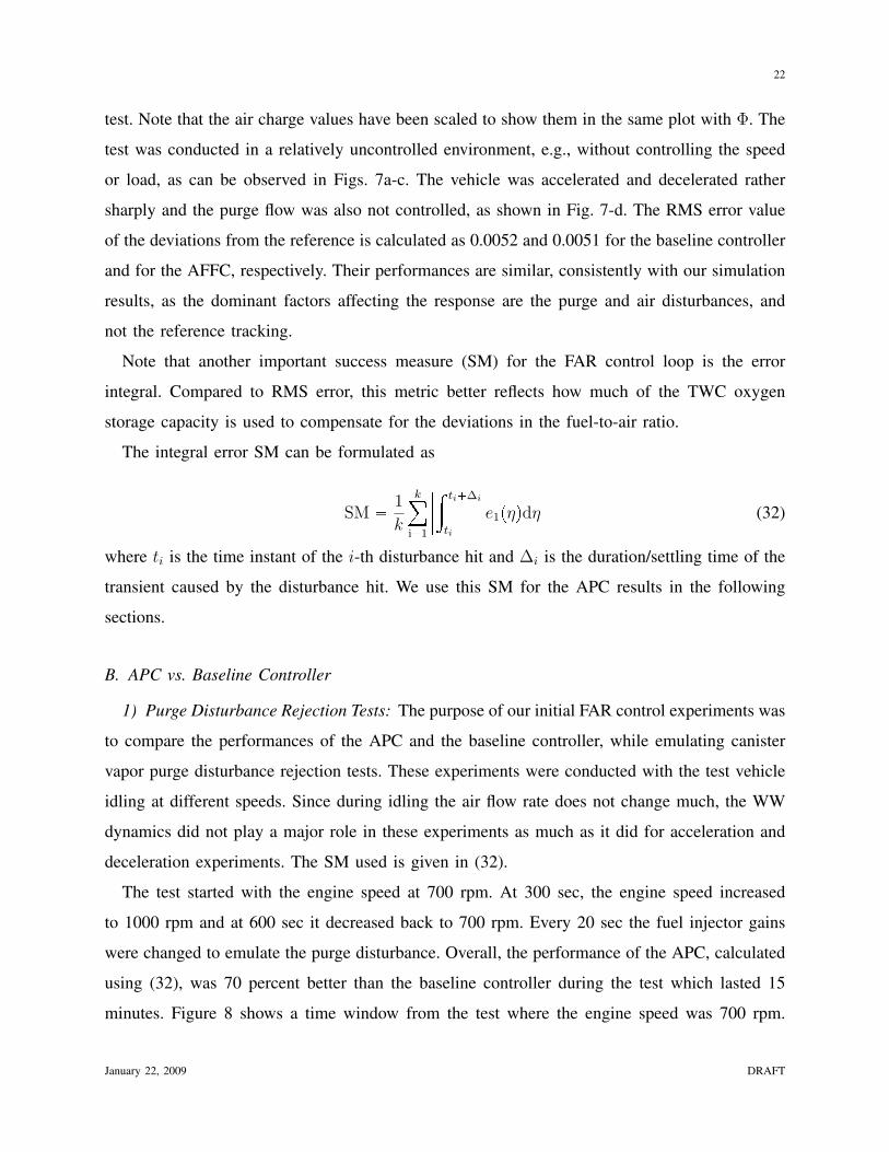
5) Anti-windup logic: The fuel injector actuators, have their hard limits and the calculated

control signal may sometimes exceed these limits, either from below or from above. Conse-


18

quently, an add-on algorithm needs to be integrated with the controller that prevents the winding

up of the integrators resulting from the adaptation laws in (17).

We use anti-windup logic where the main goal is to stop the adaptation if the control signal

saturates and if the tracking error, e1 ym yp, is not favorable. Calling the control signal

before the saturation block as u and after the saturation as usat, the anti-windup algorithm can

be expressed as in the following.

9θiptq

$'''''&'''''%

0 if u ¡ usat and e1 0

or

u usat and e1 ¡ 0

Γiie1ptqΩipt τq otherwise

(31)

The additional tracking error based condition for not suspending the adaptation during sat-

uration improved the speed of the transient response as has been demonstrated in our vehicle

experiments.

There are more rigorous anti-windup methods that are specifically developed for adaptive

controllers [39]. We plan to apply these methods in our future research.

6) Robustness: The adaptive controller design presented in Section III-C portrayed an ide-

alized situation. The delay free part of the plant dynamics, Wppsq, is assumed to be finite

dimensional, linear and time invariant with unknown parameters. It is also assumed that the

inputs and outputs to the plant can be measured exactly. However, in the real implementation,

no plant is truly linear or finite dimensional. Plant parameters may vary with time and operating

conditions, and measurements may be contaminated by noise. The plant model is almost always

approximate. It is precisely in these cases that adaptive control is most needed [37].

Due to the above possible violations of the assumptions, the controller parameters may drift

without converging to a bounded region. One of the remedies to this problem is using σ-

modification robustness scheme [37], which mainly adds a damping term to adaptation laws.

We previously used this robustness scheme in idle speed control application [40] which proved

successful and therefore we used it again in FAR control application. Please see [40] for the

details.


19

E. Final Design and Calibration

We believe that any controller design that is meant to be used in a mass-production application

must be accessible and easy to use by the engineering staff who actually implements and supports

the control strategy in production. This is particularly important given that the engineering stuff

are not expected to be highly skilled in advanced control methods. Motivated by these facts,

below we give a step by step design procedure to obtain a transparent and streamlined design. We

assume that a linear plant model with uncertain parameters and a known time delay is available.

Step 1.Select Λ and l of the signal generators defined in (13) and (14). These signal generators

act like state observers and it is suggested that the eigenvalues are selected much faster

than the reference model pole. Note that the Λ-l pair must be controllable.

Step 2.Set the initial value of the controller parameters by satisfying the model matching using

a nominal plant model.

Step 3.Set the time constant of the reference model at least two times faster than that of the

nominal plant time constant.

Step 4.Set the adaptation rate matrix Γ according to the algorithm given in (25).

Step 5.Tune the parameter c until the control requirements are satisfied. Note that increasing c

gives a tighter FAR control performance, however higher gains might cause undesired

oscillations.

Apart from these five easy steps, the design must be integrated with the robustness scheme

as discussed in Section III-D-6.

Note that the controller needs only about 0.4KB of memory for the data storage and requires

118 number of operations per computation cycle. This corresponds to less than 4 103 operations

per second. For conventional ECU’s the APC controller use around 0.04 percent of the total

computational power and that is negligible. Please see the appendix in [40] for the calculation

of the memory requirements and computational complexity.

IV. SIMULATION AND EXPERIMENTAL RESULTS

The simulation results in this section are obtained using R©Matlab and R©Simulink, and the

experimental results are obtained using a Lincoln Navigator test vehicle provided by Ford Motor

Company. The vehicle has a 5.4 liter V-8 front engine with a multi-port fuel injection system.


20

MicroAutobox

Black Oak Module

Black Oak Main Circuit Board

ATI TAB(Tool Adapter Board)

TAB

Socket

M5

Socket

ATI M5(Memory Emulator)

Laptop

running:Matlab and Control Desk and Vision

USB

dSpace

comm.

Harn

dSpaceproprietary

comm. protocol

CAN

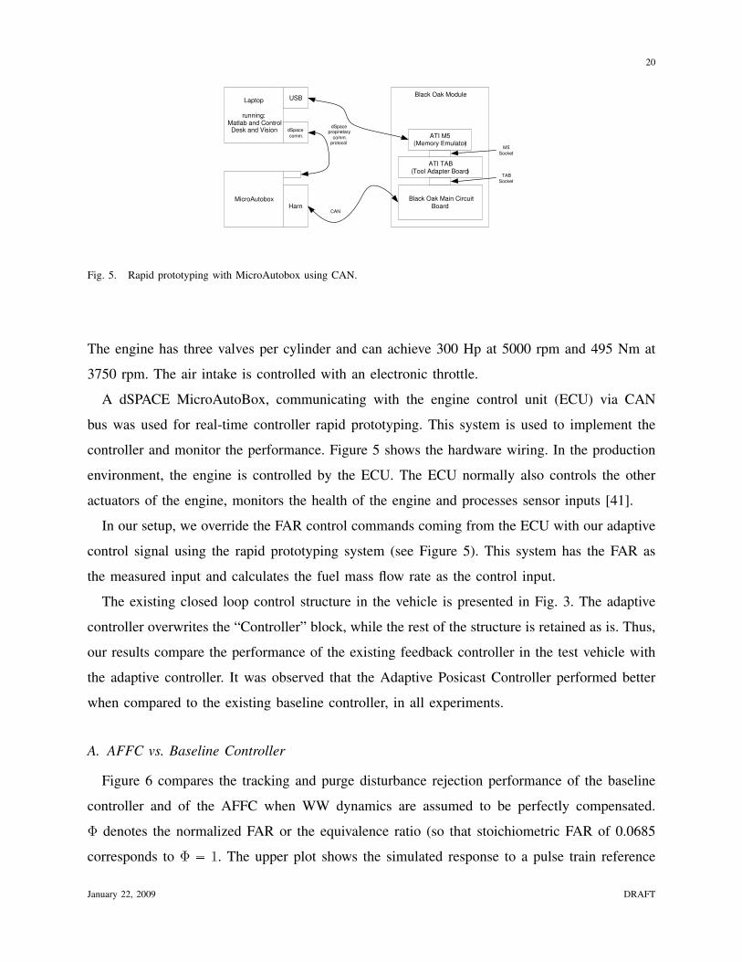
Fig. 5. Rapid prototyping with MicroAutobox using CAN.

The engine has three valves per cylinder and can achieve 300 Hp at 5000 rpm and 495 Nm at

3750 rpm. The air intake is controlled with an electronic throttle.

A dSPACE MicroAutoBox, communicating with the engine control unit (ECU) via CAN

bus was used for real-time controller rapid prototyping. This system is used to implement the

controller and monitor the performance. Figure 5 shows the hardware wiring. In the production

environment, the engine is controlled by the ECU. The ECU normally also controls the other

actuators of the engine, monitors the health of the engine and processes sensor inputs [41].

In our setup, we override the FAR control commands coming from the ECU with our adaptive

control signal using the rapid prototyping system (see Figure 5). This system has the FAR as

the measured input and calculates the fuel mass flow rate as the control input.

The existing closed loop control structure in the vehicle is presented in Fig. 3. The adaptive

controller overwrites the “Controller” block, while the rest of the structure is retained as is. Thus,

our results compare the performance of the existing feedback controller in the test vehicle with

the adaptive controller. It was observed that the Adaptive Posicast Controller performed better

when compared to the existing baseline controller, in all experiments.

A. AFFC vs. Baseline Controller

Figure 6 compares the tracking and purge disturbance rejection performance of the baseline

controller and of the AFFC when WW dynamics are assumed to be perfectly compensated.

Φ denotes the normalized FAR or the equivalence ratio (so that stoichiometric FAR of 0.0685

corresponds to Φ 1. The upper plot shows the simulated response to a pulse train reference


21

30 35 40 45 500.95

1

1.05

time [s]Φ

baseline

reference

AFFC

(a)

30 40 50 60 70 80

0.8

1

1.2

1.4

1.6

1.8

2

time [s]

Φ

baseline

reference

AFFC

(b)

Fig. 6. Comparison of baseline controller and AFFC. a) Response to a set-point change b) Response to purge disturbance.

and the lower plot shows the response to a step purge disturbance introduced at time t 30

sec and removed at time t 50 sec. It is assumed that the time delay is known to be 0.4 sec.

While designing the AFFC, the UEGO dynamics are assumed to have nominal values but then

the plant dynamics were chosen to have 20 percent deviations in high frequency gain and τm.

The baseline controller is tuned to perform well for both tracking and disturbance rejection. As

discussed before, the baseline controller cannot avoid overshoots due to the delay in the system,

while the AFFC can track the reference comparatively better. On the other hand, the disturbance

rejection capabilities are similar, since when the reference is constant, the AFFC is essentially

an integral controller.

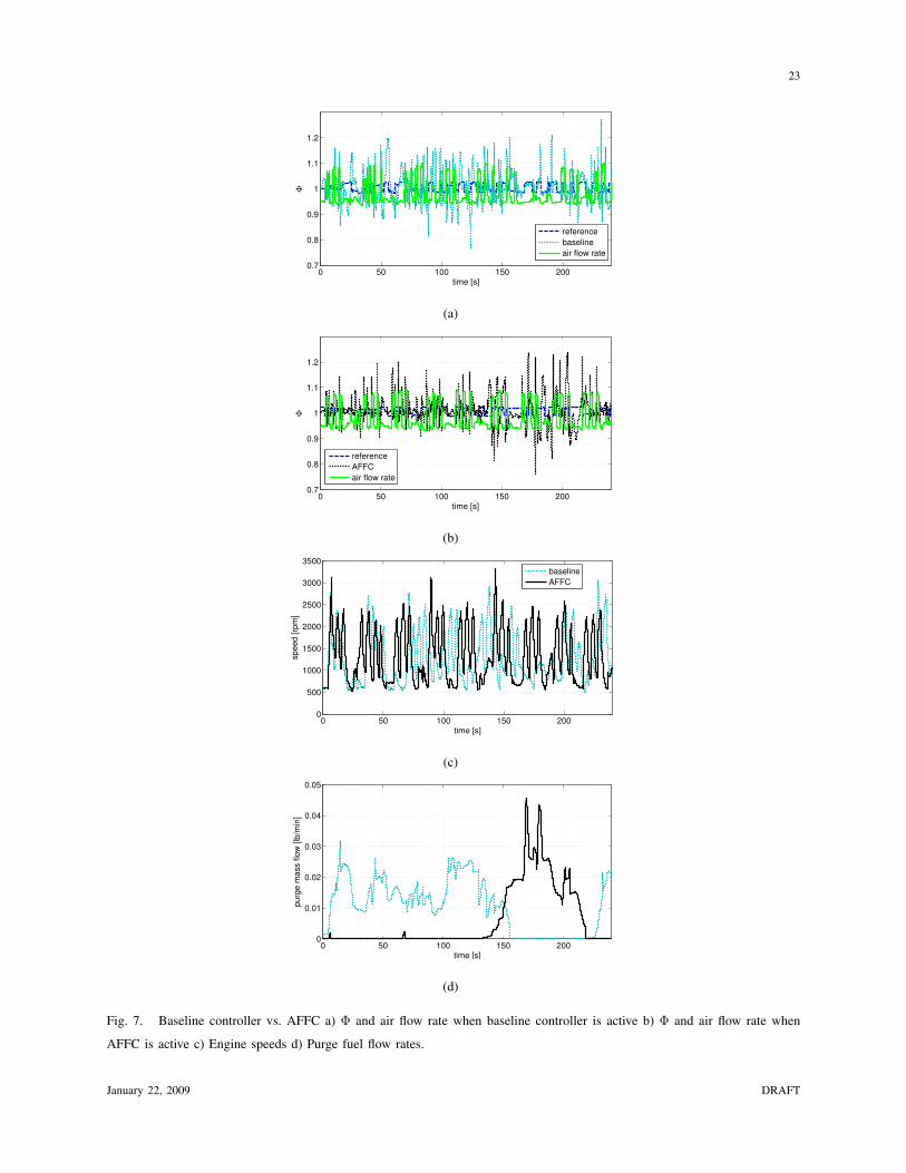
We have also tested AFFC experimentally and compared it with the existing baseline controller.

At the test time, the calibration of WW compensation was not fully completed, which allowed to

subject both controllers to challenging scenarios. Also, the time delay varied in the experiments

as opposed to the cases simulated in Fig. 6. Figure 7 shows the results from a 4-minute drive


22

test. Note that the air charge values have been scaled to show them in the same plot with Φ. The

test was conducted in a relatively uncontrolled environment, e.g., without controlling the speed

or load, as can be observed in Figs. 7a-c. The vehicle was accelerated and decelerated rather

sharply and the purge flow was also not controlled, as shown in Fig. 7-d. The RMS error value

of the deviations from the reference is calculated as 0.0052 and 0.0051 for the baseline controller

and for the AFFC, respectively. Their performances are similar, consistently with our simulation

results, as the dominant factors affecting the response are the purge and air disturbances, and

not the reference tracking.

Note that another important success measure (SM) for the FAR control loop is the error

integral. Compared to RMS error, this metric better reflects how much of the TWC oxygen

storage capacity is used to compensate for the deviations in the fuel-to-air ratio.

The integral error SM can be formulated as

SM 1

k

k

i1

» ti∆i

ti

e1pηqdη

(32)

where ti is the time instant of the i-th disturbance hit and ∆i is the duration/settling time of the

transient caused by the disturbance hit. We use this SM for the APC results in the following

sections.

B. APC vs. Baseline Controller

1) Purge Disturbance Rejection Tests: The purpose of our initial FAR control experiments was

to compare the performances of the APC and the baseline controller, while emulating canister

vapor purge disturbance rejection tests. These experiments were conducted with the test vehicle

idling at different speeds. Since during idling the air flow rate does not change much, the WW

dynamics did not play a major role in these experiments as much as it did for acceleration and

deceleration experiments. The SM used is given in (32).

The test started with the engine speed at 700 rpm. At 300 sec, the engine speed increased

to 1000 rpm and at 600 sec it decreased back to 700 rpm. Every 20 sec the fuel injector gains

were changed to emulate the purge disturbance. Overall, the performance of the APC, calculated

using (32), was 70 percent better than the baseline controller during the test which lasted 15

minutes. Figure 8 shows a time window from the test where the engine speed was 700 rpm.


23

0 50 100 150 2000.7

0.8

0.9

1

1.1

1.2

time [s]

Φ

reference

baseline

air flow rate

(a)

0 50 100 150 2000.7

0.8

0.9

1

1.1

1.2

time [s]

Φ

reference

AFFC

air flow rate

(b)

0 50 100 150 2000

500

1000

1500

2000

2500

3000

3500

time [s]

sp

ee

d [

rpm

]

baseline

AFFC

(c)

0 50 100 150 2000

0.01

0.02

0.03

0.04

0.05

time [s]

pu

rge

ma

ss f

low

[lb

/min

]

(d)

Fig. 7. Baseline controller vs. AFFC a) Φ and air flow rate when baseline controller is active b) Φ and air flow rate when

AFFC is active c) Engine speeds d) Purge fuel flow rates.


24

240 245 250 2550.85

0.9

0.95

1

1.05

time[s]

Φ [

-]

reference

baseline

APC

Fig. 8. Comparison of baseline controller with APC for purge disturbance rejection at 700 rpm.

620 625 630 6350.85

0.9

0.95

1

1.05

time[s]

Φ [

-]

reference

baseline

APC

Fig. 9. Comparison of baseline controller with APC for purge disturbance rejection at 1000 rpm, with c 1.

The APC performs considerably better, in terms of integral SM, than the baseline controller as

its features enable it to better account for the delay and achieve faster response.

Figure 9 shows how the equivalence ratio changes during the same test but now the engine

speed is 1000 rpm. Again, the performance of the APC is better than that of the baseline

controller.

2) Acceleration and Deceleration Tests: Figure 10 shows the equivalence ratio excursions

during a test in which the vehicle accelerates and then decelerates. In this case, the delay varies

with time during the test. The APC performs better overall than the baseline controller. During

the lean excursion (equivalence ratio less than 1 during acceleration), the baseline controller

appears to start the recovery from the undershoot slightly earlier than the APC. There are,

however, differences in the air flow and the equivalence ratio set-point time of increase between


25

0 1 2 3 4 5 6 7 8 9 100.8

0.9

1

1.1

1.2

a)

Φ [

-]

0 1 2 3 4 5 6 7 8 9 100

1000

2000

3000

b)

sp

ee

d [

rpm

]

0 1 2 3 4 5 6 7 8 9 100

0.2

0.4

0.6

c)

loa

d [

-]

0 1 2 3 4 5 6 7 8 9 10-0.2

-0.1

0

0.1

0.2

time [s]

d) ∫ 0t

(Φ-Φ

ref)d

t

APC

baseline

APC

Baseline

APC baseline ref(A) ref(b)

APC

baseline

Fig. 10. Time histories of a) Φ, b) Engine speed c) Engine relative air flow, d) Tracking error integral, during vehicle acceleration

and deceleration for APC vs. baseline controller, with c 1.

APC test and baseline controller test, further analysis of these suggests no real advantage for

the baseline controller over APC in terms of start of recovery timing. Note that the equivalence

ratio set-point is computed by a separate part of the engine control system in the vehicle.

For this experiment, we compared the maximum value of the integrated difference between

fuel-air equivalence ratio and its set point during the full course of the experiment. This metric

is better suited to assessing the difference between controllers for this experiment than (32)

because if one acceleration-deceleration test is assumed to be a single event, the errors cancel

each other if (32) is used, which can be observed in (10)-d. However, maximum value of the

integral relates to how much of the oxygen storage capacity is used in the worst case during

the course of the experiment. In terms of this metric, APC performs 43 percent better than the

baseline controller.

All the above experiments were conducted with the fine tuning parameter c equal to 1, which

implies that no fine-tuning was done. In Fig. 11, we present an experimental result, which shows


26

0.5 1 1.5 2 2.5 3 3.5 40.7

0.8

0.9

1

1.1

Φ [

-]

0.5 1 1.5 2 2.5 3 3.5 40.2

0.3

0.4

0.5

0.6

0.7

time [s]

loa

d [

-]

baseline1APCbaseline2

baseline (ECT=125)

APC (ECT=132)

baseline (ECT=139)

Fig. 11. Comparison of baseline controller with APC during vehicle acceleration, with c 1.5.

APC and the baseline controller performances during the vehicle acceleration, with c 1.5.

As expected, the APC outperforms the baseline controller to a greater extent compared to the

previous cases, especially on lean excursions. Note however that the load (and hence the air

charge) are less in the APC controller case in this experiment. Nevertheless, performance with

the APC is considerably better than with the baseline controller, and cannot be attributed to the

load difference between the controllers.

C. APC vs. Gain-Scheduled Smith Predictor

We compared the performance of the APC with a gain-scheduled Smith Predictor (SP). The

SP was designed based on the plant models identified at different operating points (corresponding

to different combinations of engine speeds and loads) using a relay feedback method.

Figure 12 shows the results of an acceleration-deceleration test conducted using the test vehicle.

The performances are very similar as can be seen in Fig. 12a and Fig. 12d, where the time

evolutions of Φ and the error integral is presented. On the other hand, Fig. 12c shows that the

control signal of the APC is smoother than that of the SP.

Figure 12 confirms that the adaptive controller is performing very well and similar in perfor-

mance to the Smith Predictor. Note that the gain-scheduled SP can be seen as a perfect adaptive

controller: While the APC adapts to operating point changes without the knowledge of the plant

parameters, the gain-scheduled SP uses the knowledge of the changing plant parameters that


27

0 1 2 3 4 5 6 7 80.7

0.8

0.9

1

1.1

1.2

1.3

1.4

time [s]

Φ

SP1 (ECT=123)

APC (ECT=127)

SP2 (ECT=134)

(a)

0 1 2 3 4 5 6 7 8

0.2

0.25

0.3

0.35

0.4

0.45

0.5

time [s]

loa

d [

-]

SP1

APC

SP2

(b)

0 1 2 3 4 5 6 7 8-0.6

-0.4

-0.2

0

0.2

0.4

time [s]

SP1

APC

SP2

(c)

0 1 2 3 4 5 6 7 8-0.4

-0.3

-0.2

-0.1

0

0.1

time [s]

∫ 0t(Φ

-Φre

f)dt

SP1

APC

SP2

(d)

Fig. 12. Time histories of a) Φ b) Engine relative air flow c) Feedback control input d) Tracking error integral, during vehicle

acceleration and deceleration for gain-scheduled SP vs. APC, with c 1.5.


28

need to be obtained offline by using an identification procedure for different operating points.

The adaptive controller can, in addition, adjust better to situations when plant parameters change

due to part-to-part variability or aging. For example, it is stated in [7] that due to aging or harsh

operating conditions, UEGO sensor time constant can easily increase by a factor of 10 to 20.

Also it is known that the Smith Predictor is sensitive to the delay estimation errors.

In Fig. 13, we present the simulation results that compare SP with APC. For this simulation,

the time constant for the first order system model is selected as 50 ms, which is reported in [7]

as the time constant of a state-of-the-art oxygen sensor. The nominal time delay is assumed to

be 0.4 seconds. A step input disturbance is introduced to this plant at time t 170 seconds and

the transients are plotted. The APC and the SP is tuned such that they perform similarly for

these nominal plant parameter values, in the presence of the disturbance. Then, the sensor time

constant is increased by a factor of 20 and the disturbance test is repeated. As seen in the figure,

not only the performance of the SP gets worse than the adaptive controller, but the SP response

also becomes oscillatory, which is a sign of getting closer to instability. An additional uncertainty

in the system, like a delay identification error, may cause the system to become unstable easily.

Indeed, when we introduce a delay uncertainty by increasing the nominal delay by 0.3 seconds,

we see that the loop with the SP becomes almost marginally stable. This simulation result is

presented in Fig 14.

V. SUMMARY

In this paper, we have considered the fuel-to-air ratio (FAR) control problem in port-fuel-

injection (PFI) spark-ignition (SI) engine. Two controllers, an Adaptive FeedForward Controller

(AFFC) and an Adaptive Posicast Controller (APC), have been developed and implemented in a

test vehicle. The AFFC is a simple controller based on feedforward adaptation, while the APC

is a more elaborate controller that uses adaptation in both feedforward and feedback paths and

is based on a recently developed adaptive control method for time-delay systems. The AFFC

has been shown in simulations and experiments to have better reference tracking and similar

disturbance rejection capabilities when compared to the existing baseline controller. The APC has

been shown in experiments to achieve faster recovery from disturbances and better performance

during vehicle acceleration deceleration tests. These performance improvements were a result

of various modifications and enhancements to the initial APC design, such as an algorithm to


29

170 171 172 173 174 175 176 1770.8

0.9

1

1.1

1.2

1.3

time [s]

Φ [

-]

APCSPAPC with time constant uncertaintySP with time constant uncertainty

Fig. 13. Comparison of SP and APC for input step disturbance rejection in the presence of sensor time constant uncertainty.

170 171 172 173 174 175 176 1770.8

0.9

1

1.1

1.2

1.3

time [s]

Φ [

-]

APCSPAPC with time constant and delay uncertaintySP with time constant and delay uncertainty

Fig. 14. Comparison of SP and APC for input step disturbance rejection in the presence of sensor time constant and delay

uncertainty.

handle the variable time delay, a robustness scheme and parameter initialization and fine tuning

methods. It has also been observed in our vehicle experiments that implementing APC using an

upper bound on the delay as a delay estimate assures robustness against delay variations.

In terms of applications of the APC, the FAR control problem is more challenging than the

Idle Speed Control (ISC) problem, which the authors of this paper have treated in [33] and [40],

due to a larger and variable time delay and different character of disturbances and uncertainties.

The experimental results reported here demonstrate that the APC is effective for the FAR control

problem as well.


30

APPENDIX A

DISTURBANCE REJECTION PROOF

When there is a constant disturbance d P < present in the system, the state space description

of the plant (12) is modified as

9xpptq Apxpptq bppupt τq dq, yptq hTpxpptq (33)

This in turn modifies the error equation (23) as


» 0

τ

λpt τ, σqupt τ σqdσ

krpt τq ds

e1ptq hTmeptq. (34)

Note that in FAR control application, the FAR reference, r0 P <, is constant and therefore we

have rpt τq r0 in (34). We define a new variable k1 as

k1

k d

r0

(35)

Therefore, (34) reduces to


» 0

τ

λpt τ, σqupt τ σqdσ

k1

r0s

e1ptq hTmeptq. (36)

which can also be written as

9eptq Ameptq bmrθ1T pt τqΩpt τq

» 0

τ

λpt τ, σqupt τ σqdσs

e1ptq hTmeptq. (37)

where, θ1 α1 α2 k

1

T. Equations (37) and (34) are exactly the same equations written

using different variables, meaning that the definition of the new variable does not alter the

equilibrium position of the differential equation. In addition, (37) is in the same form as in the


31

case of disturbance free system (24), and hence the stability proof follows along the same lines

and limtÑ8 e1ptq 0. Therefore, the system is stable, the disturbance is rejected and the plant

output follows the reference model output asymptotically.

To conclude, disturbance rejection is achieved by eliminating the disturbance term in the error

equation and this is done by introducing a new variable defined by shifting the feedforward

controller term k by a constant.

ACKNOWLEDGMENT

This work was supported through the Ford-MIT Alliance Initiative. The authors would like

to acknowledge Dr. Davor Hrovat of Ford Motor Company for his support and encouragement

during this project. The authors also wish to acknowledge Steve Magner and John Michelini of

Ford Motor Company for their help and valuable discussions.

REFERENCES

[1] L. Guzzella and C. H. Onder, Introduction to Modeling and Control Internal Combustion Engine Systems, 1st ed. Springer,

2004.

[2] M. Shelef and R. W. McCabe, “Twenty-five years after introduction of automotive catalysts: what next?” Catalysis Today,

vol. 62, no. 1, pp. 35–50, Sep. 2000.

[3] L. Guzzella, “Models and model-based control of IC-engines A nonlinear approach,” SAE Paper, no. 950844, 1995.

[4] B. Ault, V. K. Jones, J. D. Powell, and G. F. Franklin, “Adaptive air-fuel ratio control of a spark-ignition engine,” SAE

Paper, no. 940373, 1994.

[5] R. Turin and H. Geering, “Model-reference adaptive A/F ratio control in an SI engine based on Kalman-Filtering

techniques,” in Proc. Amer. Control Conf., 1995, pp. 4082–4090.

[6] V. K. Jones, B. A. Ault, G. F. Franklin, and J. D. Powell, “Identification and air-fuel ratio control of a spark ignition

engine,” IEEE Transactions on Control Systems Technology, vol. 3, no. 1, Mar. 1995.

[7] D. Rupp, C. Onder, and L. Guzzella, “Iterative adaptive air/fuel ratio control,” in Proc. Advances in Automotive Control,

Seascape Resort, USA, 2008.

[8] L. Guzzella, M. Simons, and H. P. Geering, “Feedback linearizing air/fuel-ratio controller,” Control Eng. Practice, vol. 5,

no. 8, pp. 1101–1105, Aug. 1997.

[9] C.-F. Chang, N. P. Fekete, A. Amstutz, and J. D. Powell, “Air-fuel ratio control in spark-ignition engines using estimation

theory,” IEEE Transactions on Control Systems Technology, vol. 3, no. 1, Mar. 1995.

[10] J. D. Powell, N. P. Fekete, and C. F. Chang, “Observer-based air-fuel ratio control,” IEEE Control Systems Magazine,

vol. 18, no. 5, pp. 72–83, Oct. 1998.

[11] S. B. Choi and J. K. Hedrick, “An observer-based controller design method for improving air/fuel characteristics of spark

ignition engines,” IEEE Transactions on Control Systems Technology, vol. 6, no. 3, pp. 325–334, May 1998.

[12] M. Won, S. B. Choi, and J. K. Hedrick, “Air-to-fuel ratio control of spark ignition engines using gaussian network sliding

control,” IEEE Transactions on Control Systems Technology, vol. 6, no. 5, pp. 678–687, Sep. 1998.


32

[13] J. K. Pieper and R. Mehrotra, “Air/fuel ratio control using sliding mode methods,” in Proc. Amer. Control Conf., San

Diego, CA, June 1999, pp. 1027–1031.

[14] J. S. Souder and J. K. Hedrick, “Adaptive sliding mode control of air-fuel ratio in internal combustion engines,” Int. J.

Robust Nonlin. Cont., vol. 14, no. 6, pp. 525–541, Apr. 2004.

[15] A. Ohata, M. Ohashi, M. Nasu, and T. Inoue, “Crank-angle domain modeling and control for idle speed,” SAE Paper, no.

950075, 1995.

[16] C. H. Onder and H. P. Geering, “Model-based multivariable speed and air-to-fuel ratio control of an si engine,” SAE Paper,

no. 930859, 1993.

[17] C. W. Vigild, K. P. H. Andersen, E. Hendricks, and M. Struwe, “Towards robust H-infinity control of an SI engine’s air/fuel

ratio,” SAE Paper, no. 1999-01-0854, 1999.

[18] L. Mianzo, H. Peng, and I. Haskara, “Transient air-fuel ratio H8 preview control of a drive-by-wire internal combustion

engine,” in Proc. Amer. Control Conf., 2001, pp. 2867–2871.

[19] S. Nakagawa, K. Katogi, and M. Oosuga, “A new air-fuel ratio feedback control for ulev/sulev standard,” SAE Paper, no.

2002-01-0194, 2002.

[20] Y.-J. Zhai and D.-L. Yu, “Neural network model-based automotive engine air/fuel ratio control and robustness evaluation,”

Engineering Applications of Artificial Intelligence, in press.

[21] K. R. Muske and C. P. J. Jones, “A model-based si engine air fuel ratio controller,” in Proc. Amer. Control Conf., 2006,

pp. 3284–3289.

[22] C. F. Chang, N. P. Fekete, and J. D. Powell, “Engine air-fuel ratio control using an event-based observer,” in Proc. of SAE,

no. 930766, 1993.

[23] A. G. Stefanopoulou, J. W. Grizzle, and J. S. Freudenberg, “Engine air-fuel ratio and torque control using secondary

throttles,” in Proc. of Conference on Decision and Control, 1994, pp. 2748–2753.

[24] Z. F., K. Grigoriadis, M. Franchek, and I. Makki, “Linear parameter varying lean burn air-fuel ratio control for a spark

ignition engine,” Journal of Dynamic Systems, Measurement and Control, vol. 129, pp. 404–414, 2007.

[25] P. Tunestal and J. K. Hedrick, “Cylinder air/fuel ratio estimation using net heat release data,” Control Eng. Practice,

vol. 11, no. 3, pp. 311–318, Mar. 2003.

[26] I. Arsie, C. Pianese, G. Rizzo, and V. Cioffi, “An adaptive estimator of fuel film dynamics in the intake port of a spark

ignition engine,” Control Eng. Practice, vol. 11, no. 3, pp. 303–309, Mar. 2003.

[27] S.-I. Niculescu and A. M. Annaswamy, “An adaptive smith-controller for time-delay systems with relative degree n ¤ 2,”

Systems and Control Letters, vol. 49, pp. 347–358, 2003.

[28] Y. Yildiz, A. Annaswamy, I. Kolmanovsky, and D. Yanakiev, “Adaptive posicast controller,” Automatica, submitted.

http://web.mit.edu/aaclab/publications/index.html.

[29] O. J. Smith, “A controller to overcome dead time,” ISA Journal, vol. 6, 1959.

[30] A. Z. Manitius and A. W. Olbrot, “Finite spectrum assignement problem for systems with delays,” IEEE Transactions on

Automatic Control, vol. 24, no. 4, 1979.

[31] K. Ichikawa, “Frequency-domain pole assignement and exact model-matching for delay systems,” International Journal

of Control, vol. 41, pp. 1015–1024, 1985.

[32] R. Ortega and R. Lozano, “Globally stable adaptive controller for systems with delay,” International Journal of Control,

vol. 47, no. 1, pp. 17–23, 1988.


33

[33] Y. Yildiz, A. Annaswamy, D. Yanakiev, and I. Kolmanovsky, “Adaptive idle speed control for internal combustion engines,”

in Proc. Amer. Control Conf., New York City, July 2007, pp. 3700–3705.

[34] ——, “Adaptive air fuel ratio control for internal combustion engines,” in Proc. Amer. Control Conf., Seattle, Washington,

June 2008, pp. 2058–2063.

[35] ——, “Automotive powertrain control problems involving time delay: An adaptive control approach,” in Proc. of ASME

Dynamic Systems and Control Conference, Ann Arbor, Michigan, Oct. 2008.

[36] S. Majhi and D. P. Atherton, “Obtaining controller parameters for a new Smith predictor using autotuning,” Automatica,

vol. 36, no. 11, pp. 1651–1658, Nov. 2000.

[37] K. S. Narendra and A. M. Annaswamy, Stable Adaptive Systems. Englewood Cliffs, NJ: Prentice-Hall, 1989.

[38] K. Engelborghs, M. Dambrine, and D. Roose, “Limitations of a class of stabilization methods for delay systems,” IEEE

Trans. Automatic Control, vol. 46, no. 2, Feb. 2001.

[39] S. P. Karason and A. M. Annaswamy, “Adaptive control in the presence of input constraints,” IEEE Trans. Automatic

Control, vol. 39, no. 11, pp. 2325–2330, Nov. 1994.

[40] Y. Yildiz, A. Annaswamy, D. Yanakiev, and I. Kolmanovsky, “Spark ignition engine idle speed control: An adaptive control

approach,” IEEE Transactions on Control Systems Technology, submitted. http://web.mit.edu/aaclab/publications/index.html.

[41] M. J. van Nieuwstadt, I. V. Kolmanovsky, P. E. Moraal, A. Stefanopoulou, and M. Jankovic, “EGR-VGT control schemes:

experimental comparison for a high-speed diesel engine,” IEEE Control Systems Magazine, vol. 20, no. 3, pp. 63–79, Jun.

2000.

PLACE

PHOTO

HERE

Yildiray Yildiz Biography text here.

PLACE

PHOTO

HERE

Anuradha Annaswamy Biography text here.


34

PLACE

PHOTO

HERE

Diana Yanakiev Biography text here.

PLACE

PHOTO

HERE

Ilya Kolmanovsky Biography text here.


Documents

1 Spark Ignition Engine Fuel-to-Air Ratio Control: An Adaptive Control Approachweb.mit.edu/aaclab/pdfs/far_012209_delete.pdf · 2009-01-24 · 1 Spark Ignition Engine Fuel-to-Air