1 Solubility Parameters — An Introductionhome.engineering.iastate.edu/~mkessler/MatE454/By_Class_Date/(8) 7...Solubility Parameters — An Introduction CONTENTS Abstract ... predicting

1 Solubility Parameters — An Introduction

CONTENTS

Abstract IntroductionHildebrand Parameters and Basic Polymer Solution ThermodynamicsHansen Solubility ParametersMethods and Problems in the Determination of Partial Solubility Parameters Calculation of the Dispersion Solubility Parameter, δD

Calculation of the Polar Solubility Parameter, δP

Calculation of the Hydrogen Bonding Solubility Parameter, δH

Supplementary Calculations and Procedures Temperature DependenceSome Special Effects Temperature ChangesEffects of Solvent Molecular SizeComputer Programs

Hansen Solubility Parameters for Water ConclusionReferences

ABSTRACTSolubility parameters have found their greatest use in the coatings industry to aid in theselection of solvents. They are used in other industries, however, to predict compatibility ofpolymers, chemical resistance, and permeation rates and even to characterize the surfaces ofpigments, fibers, and fillers. Liquids with similar solubility parameters will be miscible, andpolymers will dissolve in solvents whose solubility parameters are not too different fromtheir own. The basic principle has been “like dissolves like.” More recently, this has beenmodified to “like seeks like,” since many surface characterizations have also been made andsurfaces do not (usually) dissolve. Solubility parameters help put numbers into this simplequalitative idea. This chapter describes the tools commonly used in Hansen solubility param-eter (HSP) studies. These include liquids used as energy probes and computer programs toprocess data. The goal is to arrive at the HSP for interesting materials either by calculationor, if necessary, by experiment and preferably with agreement between the two.

INTRODUCTION

The solubility parameter has been used for many years to select solvents for coatings materials. Alack of total success has stimulated research. The skill with which solvents can be optimally selectedwith respect to cost, solvency, workplace environment, external environment, evaporation rate, flashpoint, etc. has improved over the years as a result of a series of improvements in the solubilityparameter concept and widespread use of computer techniques. Most, if not all, commercial

0-8493-7686-6/97/$0.00+$.50© 1997 by CRC Press LLC

©2000 CRC Press LLC

suppliers of solvents have computer programs to help with solvent selection. One can now easilypredict how to dissolve a given polymer in a mixture of two solvents, neither of which can dissolvethe polymer by itself.

Unfortunately, this book cannot include discussion of all of the significant efforts leading toour present state of knowledge of the solubility parameter. An attempt is made to outline develop-ments, provide some background for a basic understanding, and give examples of uses in practice.The key is to determine which affinities the important components in a system have for each other.For many products this means evaluating or estimating the relative affinities of solvents, polymers,additives, pigment surfaces, filler surfaces, fiber surfaces, and substrates.

It is noteworthy that the concepts presented here have developed toward not just predictingsolubility, which requires high affinity between solvent and solute, but to predicting affinitiesbetween different polymers leading to compatibility, and affinities to surfaces to improve dispersionand adhesion. In these applications the solubility parameter has become a tool, using well-definedliquids as energy probes, to measure the similarity, or lack of the same, of key components. Materialswith widely different chemical structure may be very close in affinities. Only those materials whichinteract differently with different solvents can be characterized in this manner. It can be expectedthat many inorganic materials, such as fillers, will not interact differently with these energy probessince their energies are very much higher. An adsorbed layer of water on the high energy surfacecan also play an important role. Regardless of these concerns, it has been possible to characterizepigments, both organic and inorganic, as well as fillers like barium sulfate, zinc oxide, etc. andalso inorganic fibers as discussed in Chapter 5. Changing the surface energies by various treatmentscan lead to a surface which can be characterized more readily and which often interacts morestrongly with given organic solvents. When the same solvents that dissolve a polymeric binder arealso those which interact most strongly with a surface, one can expect the binder and the surfaceto have high affinity for each other.

Solubility parameters are sometimes called cohesion energy parameters since they derive fromthe energy required to convert a liquid to a gas. The energy of vaporization is a direct measure ofthe total (cohesive) energy holding the liquid’s molecules together. All types of bonds holding theliquid together are broken by evaporation, and this has led to the concepts described in more detaillater. The term cohesion energy parameter is more appropriately used when referring to surfacephenomena.

HILDEBRAND PARAMETERS AND BASIC POLYMER SOLUTION THERMODYNAMICS

The term solubility parameter was first used by Hildebrand and Scott.1,2 The earlier work ofScatchard and others was contributory to this development. The Hildebrand solubility parameteris defined as the square root of the cohesive energy density:

(1.1)

V is the molar volume of the pure solvent, and E is its (measurable) energy of vaporization (seeEquation 1.15). The numerical value of the solubility parameter in MPa½ is 2.0455 times largerthan that in (cal/cm3)½. The solubility parameter is an important quantity for predicting solubilityrelations, as can be seen from the following brief introduction.

Thermodynamics requires that the free energy of mixing must be zero or negative for thesolution process to occur spontaneously. The free energy change for the solution process is givenby the relation

(1.2)

δ = ( )Ε V1 2

∆ ∆ ∆G H TSM M M= −


where ∆GM is the free energy of mixing, ∆HM is the heat of mixing, T is the absolute temperature,and ∆SM is the entropy change in the mixing process.

Equation 1.3 gives the heat of mixing as proposed by Hildebrand and Scott:

(1.3)

The ϕs are volume fractions of solvent and polymer, and VM is the volume of the mixture.Equation 1.3 is not correct. This equation has often been cited as a shortcoming of this theory inthat only positive heats of mixing are allowed. It has been shown by Patterson, Delmas, and co-workers that ∆GM

noncomb is given by the right-hand side of Equation 1.3 and not ∆GM. This isdiscussed more in Chapter 2. The correct relation is3-8

(1.4)

The noncombinatorial free energy of solution, ∆GMnoncomb, includes all free energy effects other

than the combinatorial entropy of solution occurring because of simply mixing the components.Equation 1.4 is consistent with the Prigogine corresponding states theory of polymer solutions (seeChapter 2) and can be differentiated to give expressions3,4 predicting both positive and negativeheats of mixing. Therefore, both positive and negative heats of mixing can be expected fromtheoretical considerations and have been measured accordingly. It has been clearly shown thatsolubility parameters can be used to predict both positive and negative heats of mixing. Previousobjections to the effect that only positive values are allowed in this theory are not correct.

This discussion clearly demonstrates that one should actually consider the solubility parameteras a free energy parameter. This is also more in agreement with the use of the solubility parameterplots to follow, since these use solubility parameters as axes and have the experimentally determinedboundaries of solubility defined by the condition that the free energy of mixing is zero. Thecombinatorial entropy enters as a constant factor in the plots of solubility in different solvents, forexample, since the concentrations are usually constant for a given study.

It is important to note that the solubility parameter, or rather the difference in solubilityparameters for the solvent–solute combination, is important in determining the solubility of thesystem. It is clear that a match in solubility parameters leads to a zero change in noncombinatorialfree energy, and the positive entropy change (the combinatorial entropy change) found on simplemixing to arrive at the disordered mixture compared to the pure components will ensure solutionis possible from a thermodynamic point of view. The maximum difference in solubility parameters,which can be tolerated where solution still occurs, is found by setting the noncombinatorial freeenergy change equal to the combinatorial entropy change.

(1.5)

This equation clearly shows that an alternate view of the solubility situation at the limit of solubilityis that it is the entropy change which dictates how closely the solubility parameters must matcheach other for solution to (just) occur.

It will be seen in Chapter 2 that solvents with smaller molecular volumes will be thermody-namically better than larger ones having identical solubility parameters. A practical aspect of thiseffect is that solvents with relatively low molecular volumes, such as methanol and acetone, candissolve a polymer at larger solubility parameter differences than expected from comparisons withother solvents with larger molecular volumes. An average solvent molecular volume is usuallytaken as about 100 cc/mol. The converse is also true. Larger molecular species may not dissolve,even though solubility parameter considerations might predict this. This can be a difficulty in

∆H VMM= −( )ϕ ϕ δ δ1 2 1 2

2

∆G VMMnoncomb = −( )ϕ ϕ δ δ1 2 1 2

2

∆ ∆G T SM Mcombnoncomb =


predicting the behavior of plasticizers based on data for lower molecular weight solvents only.These effects are also discussed elsewhere in this book, particularly Chapters 2, 7, and 8.

A shortcoming of the earlier solubility parameter work is that the approach was limited toregular solutions as defined by Hildebrand and Scott,2 and does not account for association betweenmolecules, such as those which polar and hydrogen bonding interactions would require. The latterproblem seems to have been largely solved with the use of multicomponent solubility parameters.However, the lack of accuracy with which the solubility parameters can be assigned will alwaysremain a problem. Using the difference between two large numbers to calculate a relatively smallheat of mixing, for example, will always be problematic.

A more detailed description of the theory presented by Hildebrand and the succession ofresearch reports which have attempted to improve on it can be found in Barton’s extensive hand-book.9 The slightly older, excellent contribution of Gardon and Teas10 is also a good source ofrelated information, particularly for coatings and adhesion phenomena. The approach of Burrell,11

who divided solvents into hydrogen bonding classes, has found numerous practical applications;the approach of Blanks and Prausnitz12 divided the solubility parameter into two components,nonpolar and “polar.” Both are worthy of mention, however, in that these have found wide use andgreatly influenced the author’s earlier activities, respectively. The latter article, in particular, wasfarsighted in that a corresponding states procedure was introduced to calculate the dispersion energycontribution to the cohesive energy. This is discussed in more detail in Chapter 2.

It can be seen from Equation 1.2 that the entropy change is beneficial to mixing. Whenmultiplied by the temperature, this will work in the direction of promoting a more negative freeenergy of mixing. This is the usual case, although there are exceptions. Increasing temperaturedoes not always lead to improved solubility relations, however. Indeed, this was the basis of thepioneering work of Patterson and co-workers,3-8 to show that increases in temperature can predict-ably lead to insolubility. Their work was done in essentially nonpolar systems. Increasing temper-ature can also lead to a nonsolvent becoming a solvent and, subsequently, a nonsolvent again withstill further increase in temperature. Polymer solubility parameters do not change much withtemperature, but those of a liquid frequently decrease rapidly with temperature. This situation allowsa nonsolvent with a solubility parameter which is initially too high to pass through a solublecondition to once more become a nonsolvent as the temperature increases. These are usually“boundary” solvents on solubility parameter plots.

The entropy changes associated with polymer solutions will be smaller than those associatedwith liquid–liquid miscibility, for example, since the “monomers” are already bound into theconfiguration dictated by the polymer they make up. They are no longer free in the sense of a liquidsolvent and cannot mix freely to contribute to a larger entropy change. This is one reason poly-mer–polymer miscibility is difficult to achieve. The free energy criterion dictates that polymersolubility parameters match extremely well for mutual compatibility, since there is little help to begained from the entropy contribution when progressively larger molecules are involved. However,polymer–polymer miscibility can be promoted by the introduction of suitable copolymers orcomonomers which interact specifically within the system. Further discussion of these phenomenais beyond the scope of the present discussion; however, see Chapter 3.

HANSEN SOLUBILITY PARAMETERS

A widely used solubility parameter approach to predicting polymer solubility is that proposed bythe author. The basis of these so-called Hansen solubility parameters (HSP) is that the total energyof vaporization of a liquid consists of several individual parts.13-17 These arise from (atomic)dispersion forces, (molecular) permanent dipole–permanent dipole forces, and (molecular) hydro-gen bonding (electron exchange). Needless to say, without the work of Hildebrand and Scott 1,2 andothers not specifically referenced here such as Scatchard, this postulate could never have beenmade. The total cohesive energy, E, can be measured by evaporating the liquid, i.e., breaking all


the cohesive bonds. It should also be noted that these cohesive energies arise from interactions ofa given solvent molecule with another of its own kind. The basis of the approach is, therefore, verysimple, and it is surprising that so many different applications have been possible since 1967 whenthe idea was first published. A rather large number of applications are discussed in this book. Othersare found in Barton.9 A lucid discussion by Barton18 enumerates typical situations where problemsoccur when using solubility parameters. These occur most often where the environment causes thesolvent molecules to interact with or within themselves differently than when they make up theirown environment, i.e., as pure liquids. Several cases are discussed where appropriate in thefollowing chapters.

Materials having similar HSP have high affinity for each other. The extent of the similarity ina given situation determines the extent of the interaction. The same cannot be said of the total orHildebrand solubility parameter.1,2 Ethanol and nitromethane, for example, have similar total sol-ubility parameters (26.1 vs. 25.1 MPa½, respectively), but their affinities are quite different. Ethanolis water soluble, while nitromethane is not. Indeed, mixtures of nitroparaffins and alcohols weredemonstrated in many cases to provide synergistic mixtures of two nonsolvents which dissolvedpolymers.13 This could never have been predicted by Hildebrand parameters, whereas the HSPconcept readily confirms the reason for this effect.

There are three major types of interaction in common organic materials. The most general arethe “non-polar” interactions. These derive from atomic forces. These have also been called disper-sion interactions in the literature. Since molecules are built up from atoms, all molecules willcontain this type of attractive force. For the saturated aliphatic hydrocarbons, for example, theseare essentially the only cohesive interactions, and the energy of vaporization is assumed to be thesame as the dispersion cohesive energy, ED. Finding the dispersion cohesive energy as the cohesionenergy of the homomorph, or hydrocarbon counterpart, is the starting point for the calculation ofthe three Hansen parameters for a given liquid. As discussed in more detail below, this is based ona corresponding states calculation.

The permanent dipole–permanent dipole interactions cause a second type of cohesion energy,the polar cohesive energy, EP. These are inherently molecular interactions and are found in mostmolecules to one extent or another. The dipole moment is the primary parameter used to calculatethese interactions. A molecule can be mainly polar in character without being water soluble, sothere is misuse of the term “polar” in the general literature. The polar solubility parameters referredto here are well-defined, experimentally verified, and can be estimated from molecular parametersas described later. As noted previously, the most polar of the solvents include those with relativelyhigh total solubility parameters which are not particularly water soluble, such as nitroparaffins,propylene carbonate, tri-n-butyl phosphate, and the like. Induced dipoles have not been treatedspecifically in this approach, but are recognized as a potentially important factor, particularly forsolvents with zero dipole moments (see the Calculation of the Polar Solubility Parameter section).

The third major cohesive energy source is hydrogen bonding, EH. This can be called moregenerally an electron exchange parameter. Hydrogen bonding is a molecular interaction and resem-bles the polar interactions in this respect. The basis of this type of cohesive energy is attractionamong molecules because of the hydrogen bonds. In this perhaps oversimplified approach, thehydrogen bonding parameter has been used to more or less collect the energies from interactionsnot included in the other two parameters. Alcohols, glycols, carboxylic acids, and other hydrophilicmaterials have high hydrogen bonding parameters. Other researchers have divided this parameterinto separate parts, for example, acid and base cohesion parameters, to allow both positive andnegative heats of mixing. These approaches will not be dealt with here, but can be found describedin Barton’s handbook9 and elsewhere.19-21 The most extensive division of the cohesive energy hasbeen done by Karger et al.22 who developed a system with five parameters — dispersion, orientation,induction, proton donor, and proton acceptor. As a single parameter, the Hansen hydrogen bondingparameter has accounted remarkably well for the experience of the author and keeps the numberof parameters to a level which allows ready practical usage.


It is clear that there are other sources of cohesion energy in various types of molecules arising,for example, from induced dipoles, metallic bonds, electrostatic interactions, or whatever type ofseparate energy can be defined. The author stopped with the three major types found in organicmolecules. It was and is recognized that additional parameters could be assigned to separate energytypes. The description of organometallic compounds could be an intriguing study, for example.This would presumably parallel similar characterizations of surface active materials, where eachseparate part of the molecule requires separate characterization for completeness. The Hansenparameters have mainly been used in connection with solubility relations mostly, but not exclusively,in the coatings industry.

Solubility and swelling have been used to confirm the solubility parameter assignments of manyof the liquids. These have then been used to derive group contribution methods and suitableequations based on molecular properties to arrive at estimates of the three parameters for additionalliquids. The goal of a prediction is to determine the similarity or difference of the cohesion energyparameters. The strength of a particular type of hydrogen bond or other bond, for example, isimportant only to the extent that it influences the cohesive energy density.

HSP do have direct application in other scientific disciplines such as surface science, wherethey have been used to characterize the wettability of various surfaces, the adsorption propertiesof pigment surfaces,10,14,16,23-26 and have even led to systematic surface treatment of inorganic fibersso they could be readily incorporated into polymers of low solubility parameters such aspolypropylene27 (see also Chapter 5). Many other applications of widely different character havebeen discussed by Barton9 and Gardon.28 Surface characterizations have not been given the attentiondeserved in terms of a unified similarity-of-energy approach. The author can certify that thinkingin terms of similarity of energy, whether surface energy or cohesive energy, can lead to rapiddecisions and plans of action in critical situations where data are lacking. In other words, theeveryday industrial crisis situation often can be reduced in scope by appropriate systematicapproaches based on similarity of energy. The successes using the HSP for surface applicationsare not surprising in view of the similarity of predictions offered by these and the Prigoginecorresponding states theory of polymer solutions discussed in Chapter 2. Flory also emphasizedthat it is the surfaces of molecules which interact to produce solutions,29 so the interactions ofmolecules residing in surfaces should clearly be included in any general approach to interactionsamong molecules.

The basic equation which governs the assignment of Hansen parameters is that the total cohesionenergy, E, must be the sum of the individual energies which make it up.

(1.6)

Dividing this by the molar volume gives the square of the total (or Hildebrand) solubility parameteras the sum of the squares of the Hansen D, P, and H components.

(1.7)

(1.8)

To sum up this section, it is emphasized that HSP quantitatively account for the cohesion energy(density). An experimental latent heat of vaporization has been considered much more reliable asa method to arrive at a cohesion energy than using molecular orbital calculations or other calcula-tions based on potential functions. Indeed, the goal of such extensive calculations for polar andhydrogen bonding molecules should be to accurately arrive at the energy of vaporization.

E E E ED P H= + +

E V E V E V E VD P H= + +

δ δ δ δ2 2 2 2= + +D P H


METHODS AND PROBLEMS IN THE DETERMINATION OF PARTIAL SOLUBILITY PARAMETERS

The best method to calculate the individual HSP depends to a great extent on what data are available.The author originally adopted an essentially experimental procedure and established values for90 liquids based on solubility data for 32 polymers.13 This procedure involved calculation of thenonpolar parameter according to the procedure outlined by Blanks and Prausnitz.12 This calcula-tional procedure is still in use and is considered the most reliable and consistent for this parameter.It is outlined below. The division of the remaining cohesive energy between the polar and hydrogenbonding interactions was initially done by trial and error to fit experimental polymer solubilitydata. A key to parameter assignments in this initial trial and error approach was that mixtures oftwo nonsolvents could be systematically found to synergistically (but predictably) dissolve givenpolymers. This meant that these had parameters placing them on opposite sides of the solubilityregion, a spheroid, from each other. By having a large number of such predictably synergisticsystems as a basis, reasonably accurate divisions into the three energy types were possible.

Using the experimentally established, approximate, δP and δH parameters, Hansen and Skaarup15

found that the Böttcher equation could be used to calculate the polar parameter quite well, and thisled to a revision of the earlier values to those now accepted for these same liquids. These valueswere also consistent with the experimental solubility data for 32 polymers available at that time andwith Equation 1.6. Furthermore, Skaarup developed the equation for the solubility parameter “dis-tance,” Ra, between two materials based on their respective partial solubility parameter components:

(1.9)

This equation was developed from plots of experimental data where the constant “4” was foundconvenient and correctly represented the solubility data as a sphere encompassing the good solvents(see Chapter 3). When the scale for the dispersion parameter is doubled compared with the othertwo parameters, essentially spherical rather than spheroidal, regions of solubility are found. Thisgreatly aids two-dimensional plotting and visualization. There are, of course, boundary regionswhere deviations can occur. These are most frequently found to involve the larger molecular speciesbeing less effective solvents compared with the smaller counterparts which define the solubilitysphere. Likewise, smaller molecular species such as acetone, methanol, nitromethane, and othersoften appear as outliers in that they dissolve a polymer even though they have solubility parametersplacing them at a distance greater than the experimentally determined radius of the solubility sphere,Ro. This dependence on molar volume is inherent in the theory developed by Hildebrand, Scott,and Scatchard discussed above. Smaller molar volume favors lower ∆GM, as discussed in Chapter 2.This in turn promotes solubility. Such smaller molecular volume species which dissolve “better”than predicted by comparisons based on solubility parameters alone should not necessarily beconsidered outliers.

The molar volume is frequently used successfully as a fourth parameter to describe molecularsize effects. These are especially important in correlating diffusional phenomena with HSP, forexample (see Chapters 7 and 8). The author has preferred to retain the three, well-defined, partialsolubility parameters with a separate, fourth, molar volume parameter, rather than to multiply thesolubility parameters by the molar volume raised to some power to redefine them.

The reason for the experimentally determined constant 4 in Equation 1.9 will be discussed inmore detail in Chapter 2. It will be noted here, however, that the constant 4 is theoretically predictedby the Prigogine corresponding states theory of polymer solutions when the geometric mean isused to estimate the interaction in mixtures of dissimilar molecules.30 This is exceptionally strongevidence that dispersion, permanent dipole–permanent dipole, and hydrogen bonding interactions

Ra D D P P H H( ) = −( ) + −( ) + −( )22 1

2

2 1

2

2 1

24 δ δ δ δ δ δ


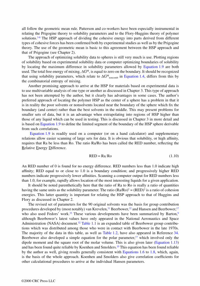
all follow the geometric mean rule. Patterson and co-workers have been especially instrumental inrelating the Prigogine theory to solubility parameters and to the Flory-Huggins theory of polymersolutions.3-8 The HSP approach of dividing the cohesive energy into parts derived from differenttypes of cohesive forces has been confirmed both by experimental studies as well as by the Prigoginetheory. The use of the geometric mean is basic to this agreement between the HSP approach andthat of Prigogine (see Chapter 2).

The approach of optimizing solubility data to spheres is still very much is use. Plotting regionsof solubility based on experimental solubility data or computer optimizing boundaries of solubilityby locating the maximum difference in solubility parameters allowed by Equation 1.9 are bothused. The total free energy of mixing, ∆GM, is equal to zero on the boundary. It should be recognizedthat using solubility parameters, which relate to ∆GM

noncomb in Equation 1.4, differs from this bythe combinatorial entropy of mixing.

Another promising approach to arrive at the HSP for materials based on experimental data isto use multivariable analysis of one type or another as discussed in Chapter 3. This type of approachhas not been attempted by the author, but it clearly has advantages in some cases. The author’spreferred approach of locating the polymer HSP as the center of a sphere has a problem in that itis in reality the poor solvents or nonsolvents located near the boundary of the sphere which fix theboundary (and center) rather than the best solvents in the middle. This may present problems forsmaller sets of data, but it is an advantage when extrapolating into regions of HSP higher thanthose of any liquid which can be used in testing. This is discussed in Chapter 3 in more detail andis based on Equation 1.9 to define the limited segment of the boundary of the HSP sphere derivablefrom such correlations.

Equation 1.9 is readily used on a computer (or on a hand calculator) and supplementaryrelations allow easier scanning of large sets for data. It is obvious that solubility, or high affinity,requires that Ra be less than Ro. The ratio Ra/Ro has been called the RED number, reflecting theRelative Energy Difference.

(1.10)

An RED number of 0 is found for no energy difference. RED numbers less than 1.0 indicate highaffinity; RED equal to or close to 1.0 is a boundary condition; and progressively higher REDnumbers indicate progressively lower affinities. Scanning a computer output for RED numbers lessthan 1.0, for example, rapidly allows location of the most interesting liquids for a given application.

It should be noted parenthetically here that the ratio of Ra to Ro is really a ratio of quantitieshaving the same units as the solubility parameter. The ratio (Ra/Ro)2 = (RED)2 is a ratio of cohesionenergies. This latter quantity is important for relating the HSP approach to that of Huggins andFlory as discussed in Chapter 2.

The revised set of parameters for the 90 original solvents was the basis for group contributionprocedures developed by (most notably) van Krevelen,31 Beerbower,32 and Hansen and Beerbower,17

who also used Fedors’ work.33 These various developments have been summarized by Barton,9

although Beerbower’s latest values have only appeared in the National Aeronautics and SpaceAdministration (NASA) document.32 Table 1.1 is an expanded table of Beerbower group contribu-tions which was distributed among those who were in contact with Beerbower in the late 1970s.The majority of the data in this table, as well as Table 1.2, have also appeared in Reference 34.Beerbower also developed a simple equation for the polar parameter,17 which involved only thedipole moment and the square root of the molar volume. This is also given later (Equation 1.13)and has been found quite reliable by Koenhen and Smolders.35 This equation has been found reliableby the author as well, giving results generally consistent with Equations 1.6 to 1.8, which, again,is the basis of the whole approach. Koenhen and Smolders also give correlation coefficients forother calculational procedures to arrive at the individual Hansen parameters.

RED Ra Ro=


TABLE 1.1

Group Contributions to Partial Solubility Parameters

Functional Group

Molar Volume,a

∆V (cm3/mol)London Parameter,

∆V δ2D (cal/mol)

Polar Parameter,∆V δ2

P (cal/mol)Electron Transfer Parameter,

∆V δ2H (cal/mol)

Total Parameter,a

∆V δ2 (cal/mol)

Aliphatic Aromaticb Alkane Cyclo Aromatic Alkane Cyclo Aromatic Aliphatic Aromatic Aliphatic Aromatic

CH –3 33.5 Same 1,125 Same Same 0 0 0 0 0 1,125 Same

CH2< 16.1 Same 1,180 Same Same 0 0 0 0 0 1,180 Same

–CH< –1.0 Same 820 Same Same 0 0 0 0 0 820 Same

>C< –19.2 Same 350 Same Same 0 0 0 0 0 350 Same

CH2 = olefin 28.5 Same 850 ± 100 ? ? 25 ± 10 ? ? 180 ± 75 ? 1,030 Same

–CH = olefin 13.5 Same 875 ± 100 ? ? 18 ± 5 ? ? 180 ± 75 ? 1,030 Same

>C = olefin –5.5 Same 800 ± 100 ? ? 60 ± 10 ? ? 180 ± 75 ? 1,030 Same

Phenyl- — 71.4 — — 7,530 — — 50 ± 25 — 50 ± 50c — 7630

C-5 ring

(saturated)

16 — — 250 — 0 0 — 0 — 250 —

C-6 ring 16 Same — 250 250 0 0 0 0 0 250 250

–F 18.0 22.0 0 0 0 1,000 ± 150 ? 700 ± 100 0 0 1,000 800b

�F2 twinf 40.0 48.0 0 0 0 700 ± 250c ? 500 ± 250c 0 0 1,700 1,360b

�F3 tripletf 66.0 78.0 0 0 0 ? ? ? 0 0 1,650 1,315b

–Cl 24.0 28.0 1,400 ± 100 ? 1,300 ± 100 1,250 ± 100 1,450 ± 100 800 ± 100 100 ± 20c Same 2,760 2,200b

�Cl2 twinf 52.0 60.0 3,650 ± 160 ? 3,100 ± 175c 800 ± 150 ? 400 ± 150c 165 ± 10c 180 ± 10c 4,600 3,670b

�Cl3 tripletf 81.9 73.9 4,750 ± 300c ? ? 300 ± 100 ? ? 350 ± 250c ? 5,400 4,300b

–Br 30.0 34.0 1,950 ± 300c 1,500 ± 175 1,650 ± 140 1,250 ± 100 1,700 ± 150 800 ± 100 500 ± 100 500 ± 100 3,700 2,960b

�Br2 twinf 62.0 70.0 4,300 ± 300c ? 3,500 ± 300c 800 ± 250c ? 400 ± 150c 825 ± 200c 800 ± 250c 5,900 4,700b

�Br3 tripletf 97.2 109.2 5,800 ± 400c ? ? 350 ± 150c ? ? 1,500 ± 300c ? 7,650 6,100b

–I 31.5 35.5 2,350 ± 250c 2,200 ± 250c 2,000 ± 250c 1,250 ± 100 1,350 ± 100 575 ± 100 1,000 ± 200c 1,000 ± 200c 4,550 3,600b

�I2 twine 66.6 74.6 5,500 ± 300c ? 4,200 ± 300c 800 ± 250c ? 400 ± 150c 1,650 ± 250c 1,800 ± 250c 8,000 6,400b

�I3 triplete 111.0 123.0 ? ? ? ? ? ? ? ? 11,700 9,350b

–O– ether 3.8 Same 0 0 0 500 ± 150 600 ± 150 450 ± 150 450 ± 25 1,200 ± 100 800 (1,650 ± 150)

>CO ketone 10.8 Same — e 2,350 ± 400 2,800 ± 325 (15, 000 ± 7%)/V 1,000 ± 300 950 ± 300 800 ± 250d 400 ± 125c 4,150 Same

–CHO (23.2) (31.4) 950 ± 300 ? 550 ± 275 2,100 ± 200 3,000 ± 500 2,750 ± 200 1,000 ± 200 750 ± 150 (4,050) Same

–COO-ester 18.0 Same — f ? — f (56,000 ± 12%)/V ? (338,000 ± 10%)/V 1,250 ± 150 475 ± 100c 4,300 Same

–COOH 28.5 Same 3,350 ± 300 3,550 ± 250 3,600 ± 400 500 ± 150 300 ± 50 750 ± 350 2,750 ± 250 2,250 ± 250c 6,600 Same


–OH 10.0 Same 1,770 ± 450 1,370 ± 500 1,870 ± 600 700 ± 200 1,100 ± 300 800 ± 150 4,650 ± 400 4,650 ± 500 7,120 Same

�(OH)2 twin

or adjacent

26.0 Same 0 ? ? 1,500 ± 100 ? ? 9,000 ± 600 9,300 ± 600 10,440 Same

–CN 24.0 Same 1,600 ± 850c ? 0 4,000 ± 800c ? 3,750 ± 300c 500 ± 200d 400 ± 125c 4,150 Same

–NO2 24.0 32.0 3,000 ± 600 ? 2,550 ± 125 3,600 ± 600 ? 1,750 ± 100 400 ± 50d 350 ± 50c 7,000 (4,400)

–NH2 amine 19.2 Same 1,050 ± 300 1,050 ± 450c 150 ± 150c 600 ± 200 600 ± 350c 800 ± 200 1,350 ± 200 2,250 ± 200d 3,000 Same

>NH2 amine 4.5 Same 1,150 ± 225 ? ? 100 ± 50 ? ? 750 ± 200 ? 2,000 Same

–NH2 amide (6.7) Same ? ? ? ? ? ? 2,700 ± 550c ? (5,850) Same

–⟩PO4 ester 28.0 Same — e ? ? (81,000 ± 10%)/V ? ? 3,000 ± 500 ? (7,000) Same

a Data from Fedors.33

b These values apply to halogens attached directly to the ring and also to halogens attached to aliphatic double-bonded C atoms.c Based on very limited data. Limits shown are roughly 95% confidence; in many cases, values are for information only and not to be used for computation.d Includes unpublished infrared data.e Use formula in ∆Vδ2

P column to calculate, with V for total compound.f Twin and triplet values apply to halogens on the same C atom, except that ∆V δ2

P also includes those on adjacent C atoms.

From Hansen, C. M., Paint Testing Manual, Manual 17, Koleske, J. V., Ed., American Society for Testing and Materials, Philadelphia, 1995, 388. Copyright ASTM. Reprinted with permission.

TABLE 1.1 (continued)Group Contributions to Partial Solubility Parameters

Functional Group

Molar Volume,a

∆V (cm3/mol)London Parameter,

∆V δ2D (cal/mol)

Polar Parameter,∆V δ2

P (cal/mol)Electron Transfer Parameter,

∆V δ2H (cal/mol)

Total Parameter,a

∆V δ2 (cal/mol)

Aliphatic Aromaticb Alkane Cyclo Aromatic Alkane Cyclo Aromatic Aliphatic Aromatic Aliphatic Aromatic


TABLE 1.2 Lydersen Group Constants

GroupAliphatic,

∆TCyclic,

∆T ∆PT

Aliphatic,∆P

Cyclic,∆P

CH3 0.020 — 0.0226 0.227 —CH2 0.020 0.013 0.0200 0.227 0.184>CH– 0.012 0.012 0.0131 0.210 0.192>C< 0.000 –0.007 0.0040 0.210 0.154�CH2 0.018 — 0.0192 0.198 —�CH– 0.018 0.011 0.0184 0.198 0.154�C< 0.000 0.011 0.0129 0.198 0.154�CH aromatic — — 0.0178 — —�CH aromatic — — 0.0149 — —

–O– 0.021 0.014 0.0175 0.16 0.12>O epoxide — — 0.0267 — —–COO– 0.047 — 0.0497 0.47 —>C�O 0.040 0.033 0.0400 0.29 0.02–CHO 0.048 — 0.0445 0.33 —–CO2O — — 0.0863 — —

–OH→ — — 0.0343 0.06 —–H→ — — –0.0077 — —–OH primary 0.082 — 0.0493 — —–OH secondary — — 0.0440 — —–OH tertiary — — 0.0593 — —–OH phenolic 0.035 — 0.0060 –0.02

–NH2 0.031 — 0.0345 0.095 —–NH– 0.031 0.024 0.0274 0.135 0.09>N– 0.014 0.007 0.0093 0.17 0.13–C�N 0.060 — 0.0539 0.36 —

–NCO — — 0.0539 — —HCON< — — 0.0546 — —–CONH– — — 0.0843 — —–CON< — — 0.0729 — —–CONH2 — — 0.0897 — —–OCONH– — — 0.0938 — —

–S– 0.015 0.008 0.0318 0.27 0.24–SH 0.015 — — — —

–Cl 1° 0.017 — 0.0311 0.320 —–Cl 2° — — 0.0317 — —Cl2 twin — — 0.0521 — —Cl aromatic — — 0.0245 — —

–Br 0.010 — 0.0392 0.50 —–Br aromatic — — 0.0313 — —

–F 0.018 — 0.006 0.224 —–I 0.012 — — 0.83 —


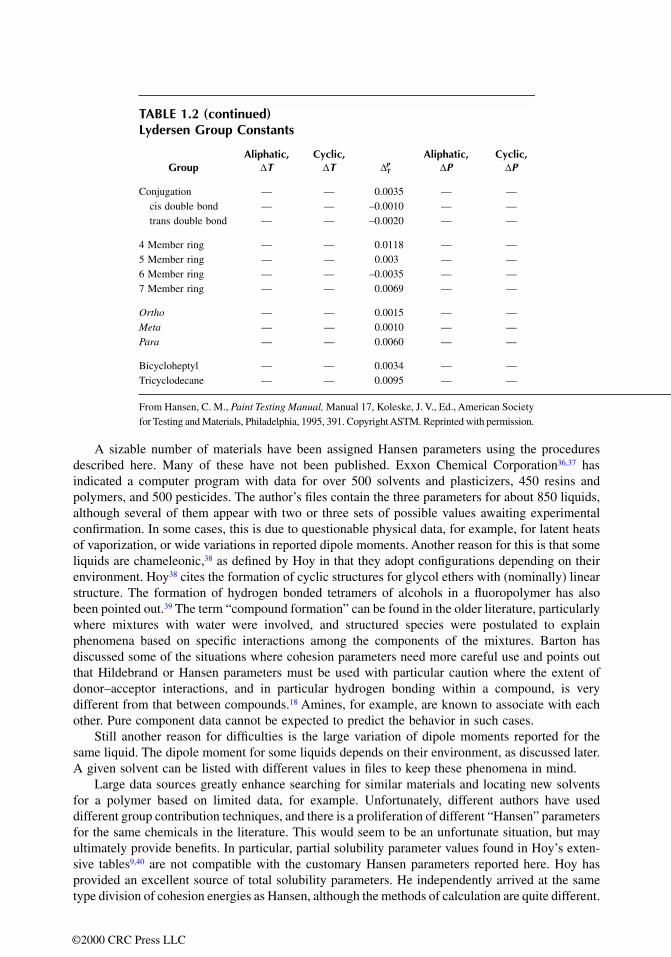
A sizable number of materials have been assigned Hansen parameters using the proceduresdescribed here. Many of these have not been published. Exxon Chemical Corporation36,37 hasindicated a computer program with data for over 500 solvents and plasticizers, 450 resins andpolymers, and 500 pesticides. The author’s files contain the three parameters for about 850 liquids,although several of them appear with two or three sets of possible values awaiting experimentalconfirmation. In some cases, this is due to questionable physical data, for example, for latent heatsof vaporization, or wide variations in reported dipole moments. Another reason for this is that someliquids are chameleonic,38 as defined by Hoy in that they adopt configurations depending on theirenvironment. Hoy38 cites the formation of cyclic structures for glycol ethers with (nominally) linearstructure. The formation of hydrogen bonded tetramers of alcohols in a fluoropolymer has alsobeen pointed out.39 The term “compound formation” can be found in the older literature, particularlywhere mixtures with water were involved, and structured species were postulated to explainphenomena based on specific interactions among the components of the mixtures. Barton hasdiscussed some of the situations where cohesion parameters need more careful use and points outthat Hildebrand or Hansen parameters must be used with particular caution where the extent ofdonor–acceptor interactions, and in particular hydrogen bonding within a compound, is verydifferent from that between compounds.18 Amines, for example, are known to associate with eachother. Pure component data cannot be expected to predict the behavior in such cases.

Still another reason for difficulties is the large variation of dipole moments reported for thesame liquid. The dipole moment for some liquids depends on their environment, as discussed later.A given solvent can be listed with different values in files to keep these phenomena in mind.

Large data sources greatly enhance searching for similar materials and locating new solventsfor a polymer based on limited data, for example. Unfortunately, different authors have useddifferent group contribution techniques, and there is a proliferation of different “Hansen” parametersfor the same chemicals in the literature. This would seem to be an unfortunate situation, but mayultimately provide benefits. In particular, partial solubility parameter values found in Hoy’s exten-sive tables9,40 are not compatible with the customary Hansen parameters reported here. Hoy hasprovided an excellent source of total solubility parameters. He independently arrived at the sametype division of cohesion energies as Hansen, although the methods of calculation are quite different.

Conjugation — — 0.0035 — —cis double bond — — –0.0010 — —trans double bond — — –0.0020 — —

4 Member ring — — 0.0118 — —5 Member ring — — 0.003 — —6 Member ring — — –0.0035 — —7 Member ring — — 0.0069 — —

Ortho — — 0.0015 — —Meta — — 0.0010 — —Para — — 0.0060 — —

Bicycloheptyl — — 0.0034 — —Tricyclodecane — — 0.0095 — —

From Hansen, C. M., Paint Testing Manual, Manual 17, Koleske, J. V., Ed., American Societyfor Testing and Materials, Philadelphia, 1995, 391. Copyright ASTM. Reprinted with permission.

TABLE 1.2 (continued)Lydersen Group Constants

GroupAliphatic,

∆TCyclic,

∆T ∆PT

Aliphatic,∆P

Cyclic,∆P


Many solvent suppliers have also presented tables of solvent properties and/or use computertechniques using these in their technical service. Partial solubility parameters not taken directlyfrom earlier well-documented sources should be used with caution. In particular, it can be notedthat the Hoy dispersion parameter is consistently lower than that found by Hansen. Hoy subtractsestimated values of the polar and hydrogen bonding energies from the total energy to find thedispersion energy. This allows for more calculational error and underestimates the dispersion energy,since the Hoy procedure does not appear to fully separate the polar and hydrogen bonding energies.The van Krevelen dispersion parameters appear to be too low. The author has not attempted thesecalculations, being completely dedicated to the full procedure based on corresponding statesdescribed here, but values estimated independently using the van Krevelen dispersion parametersare clearly low. A comparison with related compounds, or similarity principle, gives better resultsthan those found from the van Krevelen dispersion group contributions.

In the following, calculational procedures and experience are presented according to the pro-cedures found most reliable for the experimental and/or physical data available for a given liquid.

CALCULATION OF THE DISPERSION SOLUBILITY PARAMETER, dD

The δD parameter is calculated according to the procedures outlined by Blanks and Prausnitz.12

Figures 1.1, 1.2, or 1.3 can be used to find this parameter, depending on whether the molecule ofinterest is aliphatic, cycloaliphatic, or aromatic. These figures have been inspired by Barton,9 whoconverted earlier data to Standard International (SI) units. All three of these figures have beenstraight-line extrapolated into a higher range of molar volumes than that reported by Barton.Energies found with these extrapolations have also provided consistent results. As noted earlier,the solubility parameters in SI units, MPa½, are 2.0455 times larger than those in the older cgs(centimeter gram second) system, (cal/cc)½, which still finds extensive use in the U.S., for example.

FIGURE 1.1 Energy of vaporization for straight chain hydrocarbons as a function of molar volume andreduced temperature.34 (From Hansen, C. M., Paint Testing Manual, Manual 17, Koleske, J. V., Ed., AmericanSociety for Testing and Materials, Philadelphia, 1995, 389. Copyright ASTM. Reprinted with permission.)


The figure for the aliphatic liquids gives the dispersion cohesive energy, ED, whereas the othertwo figures directly report the dispersion cohesive energy density, c. The latter is much simpler touse since one need only take the square root of the value found from the figure to find the respectivepartial solubility parameter. Barton also presented a similar figure for the aliphatic solvents, but itis inconsistent with the energy figure and in error. Its use is not recommended. When substitutedcycloaliphatics or substituted aromatics are considered, simultaneous consideration of the twoseparate parts of the molecules is required. The dispersion energies are evaluated for each of thetypes of molecules involved, and a weighted average for the molecule of interest based on numbersof significant atoms is taken. For example, hexyl benzene would be the arithmetic average of thedispersion energies for an aliphatic and an aromatic liquid, each with the given molar volume ofhexyl benzene. Liquids such as chlorobenzene, toluene, and ring compounds with alkyl substitutionswith only two or three carbon atoms have been considered as cyclic compounds only. Suchweighting has been found necessary to satisfy Equation 1.6.

The critical temperature, Tc, is required to use the dispersion energy figures. If the criticaltemperature cannot be found, it must be estimated. A table of the Lydersen group contributions,41

FIGURE 1.2 Cohesive energy density for cycloalkanes as a function of molar volume and reduced temper-ature.34 (From Hansen, C. M., Paint Testing Manual, Manual 17, Koleske, J. V., Ed., American Society forTesting and Materials, Philadelphia, 1995, 389. Copyright ASTM. Reprinted with permission.)

FIGURE 1.3 Cohesive energy density for aromatic hydrocarbons as a function of molar volume and reducedtemperature.34 (From Hansen, C. M., Paint Testing Manual, Manual 17, Koleske, J. V., Ed., American Societyfor Testing and Materials, Philadelphia, 1995, 389. Copyright ASTM. Reprinted with permission.)


∆T, as given by Hoy40 for calculation of the critical temperature is included as Table 1.2. In somecases, the desired groups may not be in the table, which means some educated guessing is required.The end result does not appear too sensitive to these situations. The normal boiling temperature,Tb, is also required in this calculation. This is not always available either and must be estimatedby similarity, group contribution, or some other technique. The Lydersen group contribution methodinvolves the use of Equations 1.11 and 1.12.

(1.11)

and

(1.12)

where T has been taken as 298.15 K.The dispersion parameter is based on atomic forces. The size of the atom is important. It has

been found that corrections are required for atoms significantly larger than carbon, such as chlorine,sulfur, bromine, etc., but not for oxygen or nitrogen which have a similar size. The carbon atom inhydrocarbons is the basis of the dispersion parameter in its present form. These corrections areapplied by first finding the dispersion cohesive energy from the appropriate figure. This requiresmultiplication by the molar volume for the cyclic compounds using data from the figures here, sincethese figures give the cohesive energy densities. The dispersion cohesive energy is then increasedby adding on the correction factor. This correction factor for chlorine, bromine, and sulfur has beentaken as 1650 J/mol for each of these atoms in the molecule. Dividing by the molar volume andthen taking the square root gives the (large atom corrected) dispersion solubility parameter.

The need for these corrections has been confirmed many times, both for interpretation ofexperimental data and to allow Equations 1.6 to 1.8 to balance. Research is definitely needed inthis area. The impact of these corrections is, of course, larger for the smaller molecular species.The taking of square roots of the larger numbers involved with the larger molecular species reducesthe errors involved in these cases, since the corrections themselves are relatively small.

It can be seen from the dispersion parameters of the cyclic compounds that the ring also hasan effect similar to increasing the effective size of the interacting species. The dispersion energiesare larger for cycloaliphatic compounds than for their aliphatic counterparts, and they are higherfor aromatic compounds than for the corresponding cycloaliphatics. Similar effects also appearwith the ester group. This group appears to act as if it were, in effect, an entity which is largerthan the corresponding compound containing only carbon (i.e., its homomorph), and it has a higherdispersion solubility parameter without any special need for corrections.

The careful evaluation of the dispersion cohesive energy may not have a major impact on thevalue of the dispersion solubility parameter itself because of the taking of square roots of rather largenumbers. Larger problems arise because of Equation 1.6. Energy assigned to the dispersion portioncannot be reused when finding the other partial parameters using Equation 1.6 (or Equation 1.8). Thisis one reason group contributions are recommended in some cases as discussed below.

CALCULATION OF THE POLAR SOLUBILITY PARAMETER, dP

The earliest assignments of a “polar” solubility parameter were given by Blanks and Prausnitz.12

These parameters were, in fact, the combined polar and hydrogen bonding parameters as used byHansen, and they cannot be considered polar in the current context. The first Hansen polarparameters13 were reassigned new values by Hansen and Skaarup according to the Böttcher equa-tion.15 This equation requires the molar volume, the dipole moment (DM), the refractive index, andthe dielectric constant. These are not available for many compounds, and the calculation is somewhatmore difficult than using the much simpler equation developed by Hansen and Beerbower:17

T Tb c T T= + − ( )0 5672

. Σ∆ Σ∆

T T Tr c=


(1.13)

The constant 37.4 gives this parameter in SI units. Equation 1.13 has been consistently used by the author over the past years, particularly in

view of its reported reliability.35 This reported reliability appears to be correct. The molar volumemust be known or estimated in one way or another. This leaves only the dipole moment to be foundor estimated. Standard reference works have tables of dipole moments, with the most extensivelisting still being McClellan.42 Other data sources also have this parameter as well as other relevantparameters, and data such as latent heats and critical temperatures. The so-called DIPPR43 databasehas been found useful for many compounds of reasonably common usage, but many interestingcompounds are not included in the DIPPR. When no dipole moment is available, similarity withother compounds, group contributions, or experimental data can be used to estimate the polarsolubility parameter.

It must be noted that the fact of zero dipole moment in symmetrical molecules is not basisenough to assign a zero polar solubility parameter. An outstanding example of variations of thiskind can be found with carbon disulfide. The reported dipole moments are mostly 0 for gas phasemeasurements, supplemented by 0.08 in hexane, 0.4 in carbon tetrachloride, 0.49 in chlorobenzene,and 1.21 in nitrobenzene. There is a clear increase with increasing solubility parameter of themedia. The latter and highest value has been found experimentally most fitting for correlatingpermeation through a fluoropolymer film used for chemical protective clothing.44 Many fluoropoly-mers have considerable polarity. The lower dipole moments seem to fit in other instances. Diethylether has also presented problems as an outlier in terms of dissolving or not, and rapid permeationor not. Here, the reported dipole moments42 vary from 0.74 to 2.0 with a preferred value of 1.17,and with 1.79 in chloroform. Choosing a given value seems rather arbitrary. The chameleonic cyclicforms of the linear glycol ethers would also seem to provide for a basis of altered dipole momentsin various media.38

When Equation 1.13 cannot be used, the polar solubility parameter has been found using theBeerbower table of group contributions, by similarity to related compounds and/or by subtractionof the dispersion and hydrogen bonding cohesive energies from the total cohesive energy. Thequestion in each case is, “Which data are available and judged most reliable?” New group contri-butions can also be developed from related compounds where their dipole moments are available.These new polar group contributions then become supplementary to the Beerbower table.

For large molecules, and especially those with long hydrocarbon chains, the accurate calculationof the relatively small polar (and hydrogen bonding) contributions present special difficulties. Thelatent heats are not generally available with sufficient accuracy to allow subtraction of two largenumbers from each other to find a very small one. In such cases, the similarity and group contributionmethods are thought best. Unfortunately, latent heats found in a widely used handbook45 are notclearly reported as to the reference temperature. There is an indication that these are 25°C data,but checking indicated many of the data were identical with boiling point data reported elsewherein the literature. Subsequent editions of this handbook46 have a completely different section for thelatent heat of evaporation. Again, even moderate variations in reported heats of vaporization cancause severe problems in calculating the polar (or hydrogen bonding) parameter when Equations 1.6or 1.8 are strictly adhered to.

CALCULATION OF THE HYDROGEN BONDING SOLUBILITY PARAMETER, dH

In the earliest work, the hydrogen bonding parameter was almost always found from the subtractionof the polar and dispersion energies of vaporization from the total energy of vaporization. This isstill widely used where the required data are available and reliable. At this stage, however, the

δP DM V= ( )37 4 1 2.


group contribution techniques are considered reasonably reliable for most of the required calcula-tions and, in fact, more reliable than estimating several of the other parameters to ultimately arriveat the subtraction step just mentioned. Therefore, in the absence of reliable latent heat and dipolemoment data, group contributions are judged to be the best alternative. Similarity to relatedcompounds can also be used, of course, and the result of such a procedure should be essentiallythe same as for using group contributions.

SUPPLEMENTARY CALCULATIONS AND PROCEDURES

The procedures listed previously are those most frequently used by the author in calculating thethree partial solubility parameters for liquids where some data are available. There are a numberof other calculations and procedures which are also helpful. Latent heat data at 25°C have beenfound consistently from latent heats at another temperature using the relation given by Fishtine.47

(1.14)

This is done even if the melting point of the compound being considered is higher than 25°C. Theresult is consistent with all the other parameters, and to date no problems with particularly faultypredictions have been noted in this respect, i.e., it appears as if the predictions are not significantlyin error when experimental data have been available for checking. When the latent heat at theboiling point is given in cal/mol, Equation 1.14 is used to estimate the latent heat at 25°C. RT equalto 592 cal/mol is then subtracted from this according to Equation 1.15 to find the total cohesionenergy, E, in cgs units at this temperature:

(1.15)

A computer program has been developed by the author to assign HSP to solvents based onexperimental data alone. This has been used in several cases where the parameters for the givenliquids were desired with a high degree of accuracy. The procedure is to enter solvent quality, goodor bad, into the program for a reasonably large number of polymers where the solubility parametersand appropriate radius of interaction for the polymers are known. The program then locates thatset of δD, δP, and δH parameters for the solvent which best satisfies the requirements of a locationwithin the spheres of the appropriate polymers where solvent quality is good and outside of theappropriate spheres where it is bad.

An additional aid in estimating HSP for many compounds is that these parameters can be foundby interpolation or extrapolation, especially for homologous series. The first member may notnecessarily be a straight-line extrapolation, but comparisons with related compounds should alwaysbe made where possible to confirm assignments. Plotting the parameters for homologous seriesamong the esters, nitroparaffins, ketones, alcohols, and glycol ethers has aided in finding theparameters for related compounds.

TEMPERATURE DEPENDENCE

Only very limited attempts have been made to calculate solubility parameters at a higher temper-ature. Solubility parameter correlations of phenomena at higher temperatures have generally beenfound satisfactory when the established 25°C parameters have been used. Recalculation to highertemperatures is possible, but has not been found necessary. In this direct but approximate approach,it is assumed that the parameters all demonstrate the same temperature dependence, which, ofcourse, is not the case. It might be noted in this connection that the hydrogen bonding parameter,in particular, is the most sensitive to temperature. As the temperature is increased, more and more

∆ ∆H T H T T Tv v r r1 2 1 2

0 381 1( ) ( ) = −( ) −( )[ ] .

E E H RTv v= = −∆ ∆


hydrogen bonds are progressively weakened or broken, and this parameter will decrease morerapidly than the others.

The gas phase dipole moment is not temperature dependent, although the volume of a fluiddoes change with temperature, which will change its cohesive energy density. The change of theδD, δP, and δH parameters for liquids with temperature, T, can be estimated by the followingequations where α is the coefficient of thermal expansion:17

(1.16)

(1.17)

(1.18)

Higher temperature means a general increase in rate of solubility/diffusion/permeation, as well aslarger solubility parameter spheres. δD, δP, and δH decrease with increased temperature, as can beseen by a comparison of Equations 1.16, 1.17, and 1.18. This means that alcohols, phenols, glycols,and glycol ethers become better solvents for polymers of lower solubility parameters as thetemperature increases. Thus, increasing the temperature can cause a nonsolvent to become a goodsolvent, a fact which is often noted in practice. As mentioned earlier, it is possible that a boundarysolvent can be a good solvent at a given temperature, but become bad with either an increase intemperature or with a decrease in temperature. These phenomena are discussed in great detail byPatterson and co-workers.3,4 They can be explained either by the change in solubility parameterwith temperature or more completely by the Prigogine corresponding states theory (CST). Theeffects of temperature changes on solubility relations discussed here are most obvious with systemshaving high hydrogen bonding character. Examples are given in the next section for some specialsituations involving water and methanol.

SOME SPECIAL EFFECTS TEMPERATURE CHANGES

Water (and methanol) uptake in most polymers increases with increasing temperature. This isbecause the solubility parameters of the water and polymer are closer at higher temperatures. TheδH parameter of water (and methanol) falls with increasing temperature, while that of most polymersremains reasonably constant. Water is also well known as an exceptionally good plasticizer becauseof its small molecular size. The presence of dissolved water not only softens (reduces the glasstransition temperature) a polymer as such, but it also means diffusion rates of other species willbe increased. The presence of water in a film can also influence the uptake of other materials, suchas during solubility parameter studies or resistance testing, with hydrophilic materials being moreprone to enter the film than when the extra water is not present.

This can cause blistering on rapid cooling as discussed in Chapter 7 and in Reference 48 (seeChapters 6 and 7: Figure 6.3 shows how rapid cooling from a water-saturated state at higher tem-perature can lead to blistering; Figures 7.3 and 7.4 show how this effect can be measured experi-mentally as an increase in water content above the equilibrium value when temperature cycling isencountered). This leads to premature failure of polymeric products used in such environments.

A related problem has been encountered with methanol. It was intended to follow the rate ofuptake of methanol in an epoxy coating at room temperature by weighing coated metal panelsperiodically on an analytical balance. Blistering was encountered in the coating near the air surfaceshortly after the experiment was started. The methanol which had absorbed into the coating nearthe surface became insoluble as the temperature of the coating near the surface was lowered bythe evaporation of excess methanol during the handling and weighing of the panels. This is a rather

d dTD Dδ αδ= −1 25.

d dTP Pδ αδ= − 0 5.

d dTH Hδ δ α= − × +( )−1 22 10 0 53. .


extreme case, and, as mentioned earlier, use of the HSP determined at 25°C at elevated temperaturescan most often be done without too much trouble from a practical point of view. One should beaware that the changes in the δH parameter will be larger than those in the other parameters, andthis effect will be most significant for those liquids with larger δH values.

EFFECTS OF SOLVENT MOLECULAR SIZE

The size of both solvent and solute molecules is important for solubility, permeation, diffusion,and chemical resistance phenomena. Smaller molecules tend to be more readily soluble than largerones. As stated previously, the Hildebrand solubility parameter theory also points to smaller molarvolume solvents as being better than those with larger molar volumes, even though they may haveidentical solubility parameters.1,2 This fact of expected improved solvency for smaller moleculesis also known from the Flory-Huggins theory of polymer solutions.29 Smaller molecular solventshave also been regularly noted as being superior to those with larger molecular size when highlycrystalline polymers or solids are being tested for solubility. So it is not surprising that solventmolecular size can be an important fourth parameter in solubility and, in some cases, in chemicalresistance. Specific examples are given in Chapters 3 and 7.

The size and shape of the solvent molecule are also very important for kinetic phenomena suchas diffusion, permeation, and attainment of equilibrium. Smaller and more linear molecules diffusemore rapidly than larger and more bulky ones. The diffusion coefficient may be so low thatequilibrium is not attained for hundreds of years at room temperature in common solvent exposuresof rigid polymers like polyphenylene sulfide (PPS) with thicknesses of several millimeters.49

Likewise, the second stage in the two-stage drying process in polymer film formation by solventevaporation can last for many years.16,50 Polymer samples used for solubility parameter or othertesting may well retain solvent or monomer for many years, and this may affect the evaluations.

Attempts to include the molecular volume into a new composite solubility parameter and sizeparameter have not been particularly successful.20,21 This may be because the size effect is mostoften not caused through the thermodynamic considerations on which the solubility parameters arebased, but rather through a kinetic effect of diffusion rates or other free volume consideration. Thesimilarities in the HSP approach and the Prigogine theory discussed in Chapter 2 indicate aremarkably close, if not identical, relation between the Prigogine ρ (segment size parameter) andthe δD parameter, suggesting that molecular size differences are at least partially accounted for inthe δD parameter. The Prigogine theory also has a parameter to describe “structural effects,”including size of polymer molecules, but this has not been explored in relation to the presentdiscussion. The increase of δD with increasing molecular size among the aliphatic hydrocarbons,the higher δD values for the larger “units” represented by cycloaliphatic and aromatic rings, andthe need for corrections for larger atoms discussed earlier all tend to support this.

Sorting output data according to the molecular volume of the test solvents in a computer analysishelps to discover whether solvent molecular size is indeed an additional significant factor in a givencorrelation or testing program.

COMPUTER PROGRAMS

The author has used two computer programs extensively in his own studies and in collecting materialfor this book. These are called SPHERE and SPHERE1. They are very similar, the only differencebeing that SPHERE optimizes the polymer (or other material, of course) parameters based on allthe data, whereas SPHERE1 considers data for those solvents considered as “good” only. It neglectsthe nonsolvent data. SPHERE1 has been most useful in correlations with pigments, fillers, andfibers, as described in Chapter 5.

The data input is by solvent number followed by an indication of the quality of interactionwith that solvent. A “1” indicates a “good” solvent, while a “0” is used for a “bad” solvent. What


is considered good or bad varies according to the level of interaction being studied. This can besolution or not, a given percentage of swelling or uptake, breakthrough time being less than a giveninterval, permeation coefficients higher than a given value, long-time suspension of a pigment, etc.

The program systematically evaluates the input data using a quality of fit function called the“Desirability Function.”51 This suggestion was made by a reputed statistician many years ago as themost appropriate statistical treatment for this type of problem. It has been in use since the late 1960s.The function has the form:

(1.19)

where n is the number of solvents for which there is experimental data in the correlation. The DATAFIT approaches 1.0 as the fit improves during an optimization and reaches 1.0 when all the goodsolvents are included within the sphere and all the bad ones are outside of it.

(1.20)

The Ai for a given good solvent within the sphere and for a given bad solvent outside the sphere willbe 1.0. The error distance is the distance to the sphere boundary for the solvent in error either asbeing good and outside the sphere or being bad and inside the sphere.

Ro is the radius of the sphere, and Ra is the distance from a given solvent point to the center ofthe sphere. For a good solvent outside the sphere, an error enters the DATA FIT according to

(1.21)

Such errors are often found for solvents having low molecular volumes.For a bad solvent inside the sphere, the contribution to the DATA FIT is

(1.22)

Such errors can sometimes be found for larger molecular species such as plasticizers. This is notunexpected for the reasons mentioned earlier.

The solvents with large and/or small molecules which give the “errors” can sometimes be(temporarily) disregarded by generating a new correlation giving an excellent DATA FIT for anabbreviated range of molecular volumes. There is a special printout with the solvents arranged inorder of molecular volume which helps to analyze such situations. The computer printouts all includea column for the RED number.

The program assumes a starting point based on an average for each of the HSP for the goodsolvents only. The program then evaluates eight points at the corners of a cube, with the current bestvalues as center. Different radii are evaluated at each of these points in the optimization process.When better fits are found among the eight points, the point with the best fit is taken as a new centerand eight points around it are evaluated in a similar manner. This continues until the DATA FITcannot be improved upon. The length of the edge of the cube is then reduced in size to fine tune thefit. The initial length of the cube is 1 unit, which is reduced to 0.3 units, and finally to 0.1 units inthe final optimization step.

Experimental data for the solvents are entered with solvent number (comma) and a 1 for a goodsolvent or a 0 for a bad one.

Errors in the correlations are indicated with an “*” in the SOLUB column where the experimentalinput data are indicated. As stated above, systematic errors can sometimes be seen in the molar volume

DATA FIT A A An

n= ∗ ∗…( )1 2

1

A ei = −( )ERROR DISTANCE

A eiRo Ra= + −( )

A eiRa Ro= + −( )


printout. This may suggest a new analysis of the data. Nonsystematic errors may be real, such asfor reactions or some extraneous effect not predictable by the solubility parameter. They may alsobe bad data, and rechecking data indicated with an “*” in the output has become a routine practice.The output of this program is for the least radius allowing the maximum DATA FIT.

Results from the SPHERE program reported in this book generally include the HSP, given asD, P, and H, respectively, and Ro for the correlation in question, as well as the DATA FIT, thenumber of good solvents (G), and the total solvents (T) in the correlation. This latter informationhas not always been recorded and may be lacking for some correlations, especially the older ones.

HANSEN SOLUBILITY PARAMETERS FOR WATER

Water is such an important material that a special section is dedicated to its HSP at this point. Thebehavior of water often depends on its local environment, which makes general predictions verydifficult. Water is still so unpredictable that its use as a test solvent in solubility parameter studiesis not recommended. This is true of water as a pure liquid or water in mixtures. Table 1.3 includesdata from various HSP analyses of the behavior of water. The first set of data is derived from theenergy of vaporization of water at 25°C. The second set of data is based on a correlation of thesolubility of various solvents in water, where good solvents are soluble to more than 1% in waterand bad ones dissolve to a lesser extent. The third set of data is for a correlation of total miscibilityof the given solvents with water. The second and third entries in Table 1.3 are based on the SPHEREprogram where both good and bad solvents affect the DATA FIT and hence the result of theoptimization. The last entry in Table 1.3 is for an analysis using the SPHERE1 program. The HSPdata are for the minimum sphere which encompasses the good solvents and only the good solvents.The bad solvents are simply not considered in the data processing. This type of comparison usuallyresults in some of the parameters being lower than when all the data are included. One also hasthe problem that a considerable portion of the sphere found by the correlation covers such highenergies that no liquids have such high solubility parameters. The cohesion energy is so high asto require solids. The constant “4” in the correlations (Equation 1.9) is still used for these correla-tions, primarily based on successes at lower levels of cohesion energies, but this is also supportedby the comparison with the Prigogine corresponding states theory of polymer solutions discussedat some length in Chapter 2.

The HSP for water as a single molecule based on the latent heat at 25°C are sometimes usedin connection with mixtures with water to estimate average HSP. More recently, it has been foundin a study involving water, ethanol, and 1,2-propanediol that the HSP for water indicated by thetotal water solubility correlation could be used to explain the behavior of the mixtures involved.The averaged values are very questionable since water can associate and water has a very smallmolar volume as a single molecule. It almost appears to have a dual character. The data for the 1%correlation52 as well as for the total water miscibility suggest that about six water molecules associateinto units.

TABLE 1.3HSP Correlations Related to Water

Material dD dP dH Ro FIT G/T

Water — Single molecule 15.5 16.0 42.3 — — —Water — >1% soluble in 15.1 20.4 16.5 18.1 0.856 88/167Water — Total miscibility 18.1 17.1 16.9 13.0 0.880 47/166Water — Total miscibility “1” 18.1 12.9 15.5 13.9 1.000 47


CONCLUSION

This chapter has been dedicated to describing the tools with which different HSP characterizationscan be made and some of the pitfalls which may be encountered in the process. The justificationfor the tools is further confirmed in Chapter 2, and their use is demonstrated in all the subsequentchapters. Figure 1.4 is included to show where many common solvents are located on a δP vs. δH plot.

FIGURE 1.4 δP vs. δH plot showing the location of various common solvents. The glycols are ethyleneglycol and propylene glycol. The alcohols include methanol (M), ethanol (E), 1-butanol (B), and 1-octanol(O). The amides include dimethyl formamide (F) and dimethyl acetamide (D). The nitriles are acetonitrile(A) and butyronitrile (B). The esters are ethyl acetate (E) and n-butyl acetate (B). The amines are ethyl amine(E) and propyl amine (P). The phenols are phenol (P) and m-cresol (C). The ethers are symbolized by diethylether.


REFERENCES

1. Hildebrand, J. and Scott, R. L., The Solubility of Nonelectrolytes, 3rd Ed., Reinhold, New York, 1950.2. Hildebrand, J. and Scott, R. L., Regular Solutions, Prentice-Hall Inc., Englewood Cliffs, NJ, 1962.3. Patterson, D., and Delmas, G., New Aspects of Polymer Solution Thermodynamics, Off. Dig. Fed.

Soc. Paint Technol., 34(450), 677–692, 1962.4. Delmas, D., Patterson, D., and Somcynsky, T., Thermodynamics of Polyisobutylene-n-Alkane Sys-

tems, J. Polym. Sci., 57, 79–98, 1962.5. Bhattacharyya, S. N., Patterson, D., and Somcynsky, T., The Principle of Corresponding States and

the Excess Functions of n-Alkane Mixtures, Physica, 30, 1276–1292, 1964.6. Patterson, D., Role of Free Volume Changes in Polymer Solution Thermodynamics, J. Polym. Sci.

Part C, 16, 3379–3389, 1968.7. Patterson, D. D., Introduction to Thermodynamics of Polymer Solubility, J. Paint Technol., 41(536),

489–493, 1969.8. Biros, J., Zeman, L., and Patterson, D., Prediction of the Χ Parameter by the Solubility Parameter

and Corresponding States Theories, Macromolecules, 4(1), 30–35, 1971.9. Barton, A. F. M., Handbook of Solubility Parameters and Other Cohesion Parameters, CRC Press,

Boca Raton, FL, 1983.10. Gardon, J. L. and Teas, J. P., Solubility Parameters, in Treatise on Coatings, Vol. 2, Characterization

of Coatings: Physical Techniques, Part II, Myers, R. R. and Long, J. S., Eds., Marcel Dekker, NewYork, 1976, chap. 8.

11. Burrell, H., Solubility Parameters for Film Formers, Off. Dig. Fed. Soc. Paint Technol., 27(369),726–758, 1972; Burrell, H., A Solvent Formulating Chart, Off. Dig. Fed. Soc. Paint Technol., 29(394),1159–1173, 1957; Burrell, H., The Use of the Solubility Parameter Concept in the United States, VIFederation d’Associations de Techniciens des Industries des Peintures, Vernis, Emaux et Encresd’Imprimerie de l’Europe Continentale, Congress Book, 21–30, 1962..

12. Blanks, R. F. and Prausnitz, J. M., Thermodynamics of Polymer Solubility in Polar and NonpolarSystems, Ind. Eng. Chem. Fundam., 3(1), 1–8, 1964.

13. Hansen, C. M., The Three Dimensional Solubility Parameter — Key to Paint Component Affinities I,J. Paint Technol., 39(505), 104–117, 1967.

14. Hansen, C. M., The Three Dimensional Solubility Parameter — Key to Paint Component Affinities II,J. Paint Technol., 39(511), 505–510, 1967.

15. Hansen, C. M. and Skaarup, K., The Three Dimensional Solubility Parameter — Key to PaintComponent Affinities III, J. Paint Technol., 39(511), 511–514, 1967.

16. Hansen, C. M., The Three Dimensional Solubility Parameter and Solvent Diffusion Coefficient,Doctoral Dissertation, Danish Technical Press, Copenhagen, 1967.

17. Hansen, C. M. and Beerbower, A., Solubility Parameters, in Kirk-Othmer Encyclopedia of ChemicalTechnology, Suppl. Vol., 2nd ed., Standen, A., Ed., Interscience, New York, 1971, 889–910.

18. Barton, A. F. M., Applications of Solubility Parameters and Other Cohesion Energy Parameters, Polym.Sci. Technol. Pure Appl. Chem., 57(7), 905–912, 1985.

19. Sørensen, P., Application of the Acid/Base Concept Describing the Interaction Between Pigments,Binders, and Solvents, J. Paint Technol., 47(602), 31–39, 1975.

20. Van Dyk, J. W., Paper presented at the Fourth Chemical Congress of America, New York,August 25–30, 1991.

21. Anonymous (Note: This was, in fact, Van Dyk, J. W., but this does not appear on the bulletin), UsingDimethyl Sulfoxide (DMSO) in Industrial Formulations, Bulletin #102, Gaylord Chemical Corp.,Slidell, LA, 1992.

22. Karger, B. L., Snyder, L. R., and Eon, C., Expanded Solubility Parameter Treatment for Classificationand Use of Chromatographic Solvents and Adsorbents, Anal. Chem., 50(14), 2126–2136, 1978.

23. Hansen, C. M. and Wallström, E., On the Use of Cohesion Parameters to Characterize Surfaces,J. Adhes., 15, 275–286, 1983.

24. Hansen, C. M., Characterization of Surfaces by Spreading Liquids, J. Paint Technol., 42(550),660–664, 1970.

25. Hansen, C. M., Surface Dewetting and Coatings Performance, J. Paint Technol., 44(570), 57–60, 1972.26. Hansen, C. M. and Pierce, P. E., Surface Effects in Coatings Processes, Ind. Eng. Chem. Prod. Res.

Dev., 13(4), 218–225, 1974.


27. Hennissen, L., Systematic Modification of Filler/Fibre Surfaces to Achieve Maximum Compatibilitywith Matrix Polymers, Lecture for the Danish Society for Polymer Technology, Copenhagen,February 10, 1996.

28. Gardon, J. L., Critical Review of Concepts Common to Cohesive Energy Density, Surface Tension,Tensile Strength, Heat of Mixing, Interfacial Tension and Butt Joint Strength, J. Colloid InterfaceSci., 59(3), 582–596, 1977.

29. Flory, P. J., Principles of Polymer Chemistry, Cornell University Press, New York, 1953.30. Prigogine, I. (with the collaboration of A. Bellemans and A. Mathot), The Molecular Theory of

Solutions, North-Holland, Amsterdam, 1957, chaps. 16, 17.31. van Krevelen, D. W. and Hoftyzer, P. J., Properties of Polymers: Their Estimation and Correlation

with Chemical Structure, 2nd ed., Elsevier, Amsterdam, 1976.32. Beerbower, A., Environmental Capability of Liquids, in Interdisciplinary Approach to Liquid Lubri-

cant Technology, NASA Publication SP-318, 1973, 365–431.33. Fedors, R. F., A Method for Estimating both the Solubility Parameters and Molar Volumes of Liquids,

Polym. Eng. Sci., 14(2), 147–154, 472, 1974.34. Hansen, C. M., Solubility Parameters, in Paint Testing Manual, Manual 17, Koleske, J. V., Ed.,

American Society for Testing and Materials, Philadelphia, 1995, 383–404.35. Koenhen, D. N. and Smolders, C. A., The Determination of Solubility Parameters of Solvents and

Polymers by Means of Correlation with Other Physical Quantities, J. Appl. Polym. Sci., 19, 1163–1179,1975.

36. Anonymous, Brochure: Co-Act — A Dynamic Program for Solvent Selection, Exxon ChemicalInternational Inc., 1989.

37. Dante, M. F., Bittar, A. D., and Caillault, J. J., Program Calculates Solvent Properties and SolubilityParameters, Mod. Paint Coat., 79(9), 46–51, 1989.

38. Hoy, K. L., New Values of the Solubility Parameters from Vapor Pressure Data, J. Paint Technol.,42(541), 76–118, 1970.

39. Myers, M. M. and Abu-Isa, I. A., Elastomer Solvent Interactions III — Effects of Methanol Mixtureson Fluorocarbon Elastomers, J. Appl. Polym. Sci., 32, 3515–3539, 1986.

40. Hoy, K. L., Tables of Solubility Parameters, Union Carbide Corp., Research and Development Dept.,South Charleston, WV, 1985 (1st ed. 1969).

41. Reid, R. C. and Sherwood, T. K., Properties of Gases and Liquids, McGraw-Hill, New York, 1958.(Lydersen Method — see also Reference 31).

42. McClellan, A. L., Tables of Experimental Dipole Moments, W. H. Freeman, San Francisco, 1963.43. Tables of Physical and Thermodynamic Properties of Pure Compounds, American Institute of Chem-

ical Engineers Design Institute for Physical Property Research, Project 801, Data Compilation, R. P.Danner and T. E. Daubert, Project Supervisors, DIPPR Data Compilation Project, Department ofChemical Engineering, Pennsylvania State University, University Park.

44. Hansen, C. M., Selection of Chemicals for Permeation Testing Based on New Solubility ParameterModels for Challenge 5100 and Challenge 5200, under contract DTCG50-89-P-0333 for the U.S.Coast Guard, June 1989, Danish Isotope Centre, Copenhagen.

45. Weast, R. C., Editor-in-Chief, CRC Handbook of Chemistry and Physics, 65 ed., CRC Press, BocaRaton, FL, 1988–1989, C-672–C-683.

46. Majer, V., Enthalpy of Vaporization of Organic Compounds, in Handbook of Chemistry and Physics,72nd ed., Lide, D. R., Editor-in-Chief, CRC Press, Boca Raton, 1991–1992, 6-100–6-107.

47. Fishtine, S. H., Reliable Latent Heats of Vaporization, Ind. Eng. Chem., 55(4), 20–28, 1963; ibid. (5),55–60; ibid. (6), 47–56.

48. Hansen, C. M., New Developments in Corrosion and Blister Formation in Coatings, Prog. Org. Coat.,26, 113–120, 1995.

49. Hansen, C. M., Solvent Resistance of Polymer Composites — Glass Fibre Reinforced PolyphenyleneSulfide, Centre for Polymer Composites (Denmark), Danish Technological Institute, Taastrup, 1993,1–62, ISBN 87-7756-286-0.

50. Hansen, C. M., A Mathematical Description of Film Drying by Solvent Evaporation, J. Oil ColourChem. Assoc., 51(1), 27–43, 1968.

51. Harrington, E. C., Jr., The Desirability Function, Ind. Qual. Control, 21(10), 494–498, April 1965.52. Hansen, C. M. and Andersen B. H., The Affinities of Organic Solvents in Biological Systems, Am.

Ind. Hyg. Assoc. J., 49(6), 301–308, 1988.


Documents

1 Solubility Parameters — An Introductionhome.engineering.iastate.edu/~mkessler/MatE454/By_Class_Date/(8) 7...Solubility Parameters — An Introduction CONTENTS Abstract ... predicting