Pre-test and Post-test scores

The researcher is usually interested inseeing how well students perform un-der a variety of teaching methods, andthey have pretest scores on the stu-dents prior to the learning phase.

How should I analyze this type of data?

1. Should I enter the pretest score as a covari-ate into the model?

2. Should I just use a difference or‘improvement’ score as posttest-pretest?

3. Should I fit a split-plot analysis where a stu-dent is nested in a method and then observedat two time points (pre and post)?

1

Simulation: Comparing teaching techniquesby measuring ‘ability’ with aPretest and Posttest undertwo teaching conditions (methods)

In my simulation, I assumed we could measure Pretestscore (x-covariate) without measurement error.

The simulated true model in words:A Posttest score equals the Pretest score plus the‘mean’ gain from the method plus an error term.

The simulated true model in statistical notation:Posttesti = Pretesti + β0 + βDDgroupi + εi

Dgroup is dummy variable for trt group (0=control).β0 represents the ‘mean’ benefit of being taught

under the control method (gain over Pretest).βD represents the mean difference between the

treatment and control benefit.εi

iid∼ N(0, σ2)ε includes variability due to both Posttest measure-

ment error (we’re trying to measure ‘ability’,a latent variable) and Posttest variability amongindividuals with the same Pretest score andtreatment group.

2

Can I perceive this as a t-test on the differ-ences? i.e. Do the two groups have differentimprovements?

The true simulated model re-ordered:

Posttesti − Pretesti = β0 + βDDgroupi + εi

which is the same as...

Diffi = µ + αgroupi + εi

THAT’S A T-TEST ON THE DIFFERENCES!!

3

Simulated valuesn=100 with 50 in each treatment group.

Pretest scores randomly generated from N(60, 102).

Mean benefit from being in control group = 12.

Mean benefit from being in treatment group = 20.

And σ = 5.65

Pretest score (baseline information) disappears in the differences.Plot of the differences:

group (jittered)

improvement

-10

010

2030

40

Control Treatment

> t.test((posttest-pretest)~trt,var.equal=TRUE)

Two Sample t-test

data: (posttest - pretest) by trt

t = -6.5223, df = 98, p-value = 3.042e-09

alternative hypothesis: true difference in means is not equal to 0

95 percent confidence interval:

-10.189924 -5.435674

sample estimates:

mean in group 1 mean in group 2

11.65641 19.46921

4

Can I perceive this as an ANCOVA model?The true simulated model re-ordered:

Posttesti = β0 + 1 ∗ Pretesti + βDDgroupi + εi(baseline covariate)

Looks like an ANCOVA with parallel lines among groups (no interac-

tion term between pretest and group) and a covariate slope coefficient

forced to be a 1.

Fitted ANCOVA below (no restriction on covariate coefficient):

40 50 60 70 80

4050

6070

8090

100

simulated data set with fitted full model

pretest

posttest

controltreatment

ANCOVA model output:

> lm.out.add=lm(posttest~trt+pretest)

> summary(lm.out.add)

Coefficients:

Estimate Std. Error t value Pr(>|t|)

(Intercept) 7.42934 3.89922 1.905 0.0597 .

trt2 7.89301 1.19862 6.585 2.34e-09 ***

pretest 1.07070 0.06366 16.819 < 2e-16 ***

NOTE: pretest coefficient not significantly different than 1, tobs = 1.11, pvalue=0.2697):

5

Any difference in ANCOVA and t-test results?1000 simulations under HA: Record t-test for treatment

t-test p-values vs. ANCOVA p-values (treatment effect):

2 4 6 8 10 12

24

68

1012

ancova: -log10(pvalue)

ttest

: -lo

g10(

pval

ue)

-log10(pvalue): larger=> more significant

80.5 % hadsmaller pvalue in ANCOVA

The point (8,5) is used for pvalues (10^-8,10^-5)

OLS estimates and standard errors in ANCOVA.

In t-test, difference in improvement divided by√

σ2

50 + σ2

50

Not exactly the same results, but strongly correlated.

6

Estimated Treatment effect:ANCOVA

Treatment effect estimates

Frequency

0 2 4 6 8 10 12 14

050

150

250

ttest

Treatment effect estimates

Frequency

0 2 4 6 8 10 12 14

050

100

200

Another ANCOVA output example (coefficient NOT forced to be 1):

> lm.out.add=lm(posttest~trt+pretest)

Coefficients:

Estimate Std. Error t value Pr(>|t|)

(Intercept) 2.2208 36.8012 0.060 0.952

trt2 8.3796 1.2446 6.733 1.18e-09 ***

pretest 1.1668 0.6132 1.903 0.060 .

Residual standard error: 6.184 on 97 degrees of freedom

Multiple R-squared: 0.351,Adjusted R-squared: 0.3376

F-statistic: 26.23 on 2 and 97 DF, p-value: 7.835e-10

NOTE: pretest coefficient not significantly different than 1, tobs = 0.332, pvalue=0.0.7406):

7

What about Type I error rate in ANCOVA?

For how the data were simulated, this a model mis-specification.Is the ANCOVA declaring significance too often?

1000 simulations underH0 with no teaching method effect.

Proportion of times effectdeclared significant using

p = 0.05 cut-off

ANCOVA ttest split-plot0.049 0.043 0.043

treatment pvalues for ANCOVA (B=1000)

pvalues

Frequency

0.0 0.2 0.4 0.6 0.8 1.0

010

2030

4050

60

treatment pvalues for ttest (B=1000)

pvalues

Frequency

0.0 0.2 0.4 0.6 0.8 1.0

010

2030

4050

60

Looks OK, but I think I would personally still recom-mend t-test on differences or split-plot analysis (next) asthese models test for the effect of interest in a way that isconsistent with how I perceived the data were generated.

8

The ANCOVA model (parallel lines):

Posttest = β0 + β1Pretest + βDDgroup + ε

As we saw before, if we force β1 = 1 in this ANCOVA,then this is the exact same testing for treatment (i.e. pvalue)as a difference in improvement between the two groups.

What does forcing β1 = 1 imply in the ANCOVA?A 1 point increase in Pretest score is associatedwith a 1 point increase in Posttest score (on average).

Seems like setting β1 = 1 is at least reasonable.

What does excluding interaction Pretest∗Dgroup imply?A 1 point increase in Pretest score must have thesame impact on Posttest score for both groups.

Overall, as long as you do not have reason to believe that the slope

for Pretest should differ between groups and a 1 point increase in

Pretest coincides with a 1 point increase in Posttest, then the t-test

on differences seems most straight-forward when testing for treat-

ment effect.

But if these assumptions are questionable, we can use ANCOVA with

interaction to give a more flexible model.

9

Can I perceive this as a split-plot model?

Student is nested in a treatment group, and we observethe student at two time points.

Example:

6065

7075

80

Interaction plot (from split plot)

time

score

pre post

controltreatment

If students are randomly assigned to treatment group, weexpect no difference between the groups at the first timepoint. If there is a teaching method effect, we expect tosee an interaction between treatment group and time.

In other words, we’re looking to see if the difference be-tween the pre and post scores differs across treatmentgroups.

10

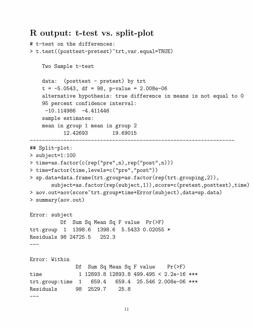
R output: t-test vs. split-plot# t-test on the differences:

> t.test((posttest-pretest)~trt,var.equal=TRUE)

Two Sample t-test

data: (posttest - pretest) by trt

t = -5.0543, df = 98, p-value = 2.008e-06

alternative hypothesis: true difference in means is not equal to 0

95 percent confidence interval:

-10.114986 -4.411446

sample estimates:

mean in group 1 mean in group 2

12.42693 19.69015

-------------------------------------------------------------------

## Split-plot:

> subject=1:100

> time=as.factor(c(rep("pre",n),rep("post",n)))

> time=factor(time,levels=c("pre","post"))

> sp.data=data.frame(trt.group=as.factor(rep(trt.grouping,2)),

subject=as.factor(rep(subject,1)),score=c(pretest,posttest),time)

> aov.out=aov(score~trt.group*time+Error(subject),data=sp.data)

> summary(aov.out)

Error: subject

Df Sum Sq Mean Sq F value Pr(>F)

trt.group 1 1398.6 1398.6 5.5433 0.02055 *

Residuals 98 24725.5 252.3

---

Error: Within

Df Sum Sq Mean Sq F value Pr(>F)

time 1 12893.8 12893.8 499.495 < 2.2e-16 ***

trt.group:time 1 659.4 659.4 25.546 2.008e-06 ***

Residuals 98 2529.7 25.8

---

11

1000 simulations: split-plot p-values (interaction) vs.t-test p-values (on differences)

2 4 6 8 10 12 14

24

68

1012

14

ttest: -log10(pvalue)

split

plot

: -lo

g10(

pval

ue)

-log10(pvalue): larger=> more significant

These are doing the same test.

12

But, as always, listen to your client and be understandingof the things that are commonly used and accepted (andeven expected) within each discipline.

In this case, the t-test on the differences and theANCOVA give results that are fairly similar. So, if they’remost comfortable with using a pre-test score as baselinecovariate, then that’s how I would proceed. And in the ed-ucation discipline, I believe the ANCOVA model is com-mon.

NOTE: The covariate used in the ANCOVA is commonly centered

in order to give a nice interpretation of the intercept. When Pretest

is centered, β0 is the mean Posttest score for the baseline group at

the ‘average’ Pretest score.

13