1

Sequential VAE-LSTM for AnomalyDetection on Time Series

Run-Qing Chen, Guang-Hui Shi, Wan-Lei Zhao, Chang-Hui Liang

Abstract—In order to support stable web-based applications and services, anomalies on the IT performance status have to be detectedtimely. Moreover, the performance trend across the time series should be predicted. In this paper, we propose SeqVL (SequentialVAE-LSTM), a neural network model based on both VAE (Variational Auto-Encoder) and LSTM (Long Short-Term Memory). Thiswork is the first attempt to integrate unsupervised anomaly detection and trend prediction under one framework. Moreover, this modelperforms considerably better on detection and prediction than VAE and LSTM work alone. On unsupervised anomaly detection, SeqVLachieves competitive experimental results compared with other state-of-the-art methods on public datasets. On trend prediction, SeqVLoutperforms several classic time series prediction models in the experiments of the public dataset.

Index Terms—Time series, Unsupervised anomaly detection, Robust Trend prediction.

F

1 INTRODUCTION

Due to the steady growth of cloud computing and the widespread of various web services, a big volume of IT operationdata are generated on the daily basis. IT operations ana-lytics are introduced to discover patterns from these hugeamounts of time series data. The primary goal of operationsanalytics is to automate or monitor IT systems based on theoperation data via artificial intelligence. It is widely knownas artificial intelligence for IT operations (AIOps). Two fun-damental tasks in AIOps are trend prediction and anomalydetection on the key performance indicators (KPIs), suchas the time series about the number of user accesses andmemory usage, etc.

In general, a sequence of KPIs is given as a univariatetime seriesX = {x1, · · · , xt, xt+1, · · · , xn−1, xn}, where thesubscript represents the time stamp and xt is the real-valuedstatus at one time stamp. The trend prediction is to estimatestatus xt+1 given the status from 1 to t are known. Whileanomaly detection is to judge the status on time stamp tis abnormal given the status across all t time stamps areknown. In practice, these two tasks are expected to workjointly to undertake automatic performance monitoring onthe KPIs. Most of the KPIs are the reflections of the userbehaviors, habits, and schedule [1]. Since these events arelargely repeated periodically, the KPI sequences are mostlystationary and periodic on the daily or weekly basis. There-fore they are believed predictable though the latent factorsthat impact the status are hard to be completely revealed.

Although KPIs largely exhibit regular patterns, theyare mixed with noises. As a result, performing anomalydetection and trend prediction on these time series are non-trivial in practice. First of all, it is unrealistic to expect a large

• Run-Qing Chen, Chang-Hui Liang and Wan-Lei Zhao are with XiamenUniversity, Fujian Key Laboratory of Sensing and Computing for SmartCity, Xiamen University, Fujian, China. E-mail: wlzhao@xmu.edu.cn

• Guang-Hui Shi is with Bonree Inc., Beijing, China

number of labeled data available to train anomaly detectionmodels. On the one hand, KPIs are in big amount whilethe abnormal status are relatively in a rare occurrence. Onthe other hand, both the regular patterns of KPIs and theappearance of abnormal status drift as time goes on. Anno-tating big amount of training data therefore would requirepainstaking efforts and is error-prone. As a result, unsuper-vised anomaly detection is preferred. Moreover, due to thepresence of anomalies in the KPIs, the popular predictionmodels such as long short-term memories (LSTMs) [2],[3] which perform well in the ideal environment fail toreturn decent results. For this reason, the robustness of theprediction model is highly valued.

There is a rich body of works for both unsupervisedanomaly detection and robust trend prediction in the recentliterature. Due to the great success of deep learning in manytasks, it has been recently introduced into both unsuper-vised anomaly detection and robust trend prediction. In thestate-of-the-art works, these two tasks are addressed sepa-rately. Generative models such as variational auto-encoders(VAEs) [4] are adopted in anomaly detection. The timeseries are sliced into windows of equal size and time statuswithin each window are encoded [1], [5]. Abnormal status isidentified as it is far apart from the decoded normal status.Encouraging results are achieved from these approaches [1],[5]. Unfortunately, the performance turns out to be un-stable as it ignores the temporal relationship between thesliding windows during the encoding. Typically, LSTM isadopted [2], [3] in the trend prediction. The advantage isthat LSTM is able to capture the latent correlations betweenlong term and short term status along the time series,even such correlation is non-linear. Due to its high modelcomplexity, it is unfortunately sensitive to anomalies andnoises. The problem is alleviated by ensemble learning [6],[7], nevertheless several folds of computational overheadbecome inevitable.

Different from existing solutions, a joint model calledSequential VAE-LSTM (SeqVL) is proposed in this paper. In

arX

iv:1

910.

0381

8v2

[cs

.LG

] 1

0 O

ct 2

019

2

our solution, VAE and LSTM are integrated as a whole toaddress both unsupervised anomaly detection and robusttrend prediction. The advantages of such framework are atleast two folds.

• Firstly, VAE is adopted for unsupervised anomalydetection. LSTM block in SeqVL propagates the se-quential patterns latent across neighboring windowsto the VAE block during the training. The tempo-ral relationships between the windows, which havebeen missed in existing VAE-based detection ap-proaches, are therefore supplied to the VAE block.

• Secondly, LSTM is adopted for trend prediction.LSTM takes the re-encoded time series from theoutput of the anomaly detection (VAE block). Suchdesign considerably reduces the impact of abnormaldata and noises on the trend prediction block.

As a result, the prediction block (LSTM) makes use ofthe clean input from VAE. Meanwhile, the detection block(VAE) is trained with time series segments across whichthe sequential order is maintained by LSTM. This leads toconsiderably better performance than using LSTM and VAEalone for either anomaly detection or trend prediction on IToperations.

The remainder of this paper is organized as follows.Related works about unsupervised anomaly detection andtrend prediction are presented in Section 2. The proposedmodel, namely SeqVL is presented in Section 3. The ef-fectiveness of our approach both for trend prediction andanomaly detection is studied on two datasets in Section 4.Finally, Section 5 concludes the paper.

2 RELATED WORK

2.1 Trend Prediction on Time SeriesTrend prediction on the time series is an old topic as wellas a new subject. On the one hand, it is an old topic in thesense it could be traced back to nearly 100 years ago [8]. Insuch a long period, classic approaches such as ARIMA [9],[10], Kalman Filter [11] and Holt-Winters [12] were pro-posed one after another. The implementations about theseclassic algorithms are found from recent packages suchas Prophet [13] and hawkular [14]. Although efficient, theunderlying patterns usually underfit due to their low modelcomplexity. On the other hand, this is a new issue in thesense the steady growth of the big volume of IT operationdata, which are mixed noises and anomalies, impose newchallenges to this century-old issue.

Recently LSTMs is adopted for trend prediction for itssuperior capability of capturing long-term patterns on tem-poral data [6], [7]. In [6], [7], multiple prediction modelsare trained from one time series, the prediction is madeby ensembling multiple predictions into one. The LSTMsmodel is also modified to performing online trend predic-tion in [15]. It allows the learnt model to be adaptive toemerging patterns of time series by balancing the weightsbetween the come-in status and historical status.

2.2 Unsupervised Anomaly Detection on Time SeriesIT operations data are in big amount and the anomalies arepresent in different patterns from one time series to another.

It is therefore infeasible to train the detection model in asupervised manner. For this reason, the research focus inthe literature is on unsupervised anomaly detection.

The first category of approaches is built upon the trendprediction. Specifically, when the status is far apart from thepredicted status value at one time stamp, it is considered asan anomaly. In [16], ARIMA is adopted for trend prediction,then the detection is made based on the predicted status.However, due to poor prediction performance from ARIMA,precise anomaly detection is not achievable. Recently, dueto its good capability in capturing patterns from time se-ries with lags of unknown duration, a stacked LSTM [17]is proposed to perform anomaly detection. However, theuncertainty of the prediction model itself is overlooked inthe approach. To address this issue, Research from Uberintroduced Bayesian networks into LSTM auto-encoder. MCdropout is adopted to estimate the prediction uncertaintyof the LSTM auto-encoder [18], [19]. In addition to theuncertainty of the prediction model, historical predictionerrors is considered in a recent approach from NASA [20].Nevertheless, all these detectors rely on largely the per-formance of the trend prediction. Inferior performance isobserved when the time series show drifting patterns.

Another type of detection approaches divides the timeseries into a series of segments via a sliding window. Thenconventional outlier detection approaches such as one-classSVM [21], [22] or SR [23] are adopted for anomaly detectionwithin each window. Considering the patterns from boththe regular status and the anomalies drift as time goeson, iForest [24] and robust random cut forest (RRCF) [25]are proposed. The latter reduces detection false positivesconsiderably. Recently SPOT and DSPOT are proposed [26]to distinguish the anomalies from regular patterns with anadaptive threshold based on Extreme Value Theory [27]. Asthe anomalies are under different distribution from normalstatus, VAE is adopted to encode the regular patterns ineach window [1]. The performance of VAE based approachis further boosted with an adversarial training [5].

In the above detection approaches, the temporal relation-ship between the windows is ignored. In the training, seg-ments are treated independently and are shuffled randomly.Different from [1], [5], our joint model SeqVL maintains thesequential order between segments due to the incorporationof LSTM block.

3 THE PROPOSED MODEL

In this section, a framework that integrates LSTM andVAE for both trend prediction and anomaly detection ispresented.

3.1 Data Preprocessing

Given a raw operations time sequence R ={r1, · · · , rt, · · · , rn}, it is not unusual that the operationstatus are missing on some time stamps due to suddenserver down or network crash. Conventionally, themissing values are either simply filled with zeros or withaverage/median of all the status. Another common practiceis to perform the linear interpolation with adjacent status.These schemes are effective when the missing status are

3

0

2

#104

A B

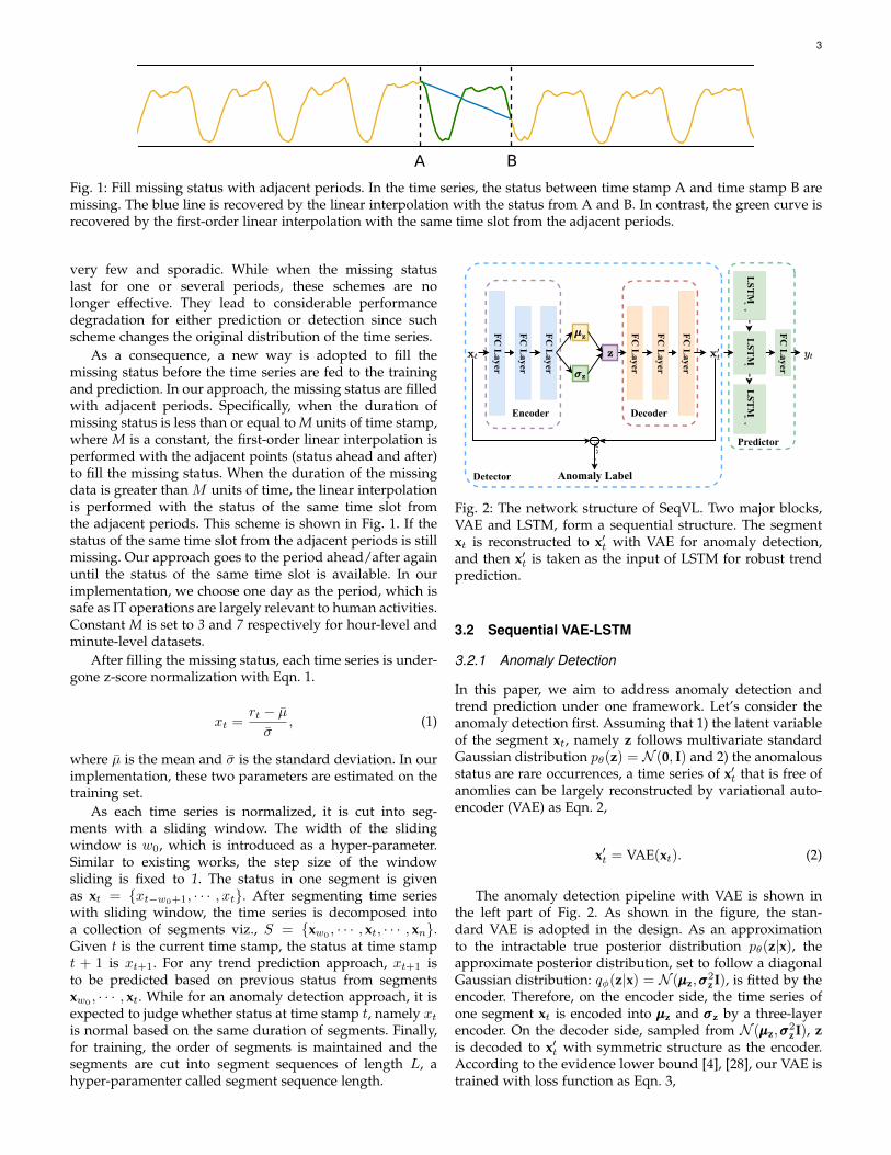
Fig. 1: Fill missing status with adjacent periods. In the time series, the status between time stamp A and time stamp B aremissing. The blue line is recovered by the linear interpolation with the status from A and B. In contrast, the green curve isrecovered by the first-order linear interpolation with the same time slot from the adjacent periods.

very few and sporadic. While when the missing statuslast for one or several periods, these schemes are nolonger effective. They lead to considerable performancedegradation for either prediction or detection since suchscheme changes the original distribution of the time series.

As a consequence, a new way is adopted to fill themissing status before the time series are fed to the trainingand prediction. In our approach, the missing status are filledwith adjacent periods. Specifically, when the duration ofmissing status is less than or equal to M units of time stamp,where M is a constant, the first-order linear interpolation isperformed with the adjacent points (status ahead and after)to fill the missing status. When the duration of the missingdata is greater than M units of time, the linear interpolationis performed with the status of the same time slot fromthe adjacent periods. This scheme is shown in Fig. 1. If thestatus of the same time slot from the adjacent periods is stillmissing. Our approach goes to the period ahead/after againuntil the status of the same time slot is available. In ourimplementation, we choose one day as the period, which issafe as IT operations are largely relevant to human activities.Constant M is set to 3 and 7 respectively for hour-level andminute-level datasets.

After filling the missing status, each time series is under-gone z-score normalization with Eqn. 1.

xt =rt − µσ

, (1)

where µ is the mean and σ is the standard deviation. In ourimplementation, these two parameters are estimated on thetraining set.

As each time series is normalized, it is cut into seg-ments with a sliding window. The width of the slidingwindow is w0, which is introduced as a hyper-parameter.Similar to existing works, the step size of the windowsliding is fixed to 1. The status in one segment is givenas xt = {xt−w0+1, · · · , xt}. After segmenting time serieswith sliding window, the time series is decomposed intoa collection of segments viz., S = {xw0

, · · · , xt, · · · , xn}.Given t is the current time stamp, the status at time stampt + 1 is xt+1. For any trend prediction approach, xt+1 isto be predicted based on previous status from segmentsxw0

, · · · , xt. While for an anomaly detection approach, it isexpected to judge whether status at time stamp t, namely xtis normal based on the same duration of segments. Finally,for training, the order of segments is maintained and thesegments are cut into segment sequences of length L, ahyper-paramenter called segment sequence length.

FC L

ayer

FC L

ayer

FC L

ayer

FC L

ayer

FC L

ayer

FC L

ayer

z

μμz

σσz

x′t

Encoder Decoder

xt

LST

Mt

FC L

ayer

yt

LST

Mt−

1L

STM

t+1

Predictorkσ

r

Anomaly LabelDetector

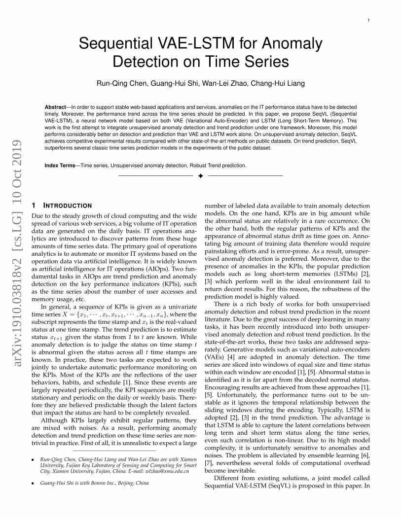
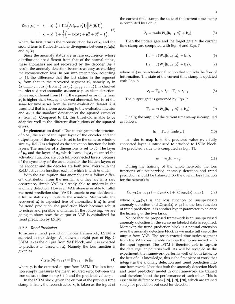
Fig. 2: The network structure of SeqVL. Two major blocks,VAE and LSTM, form a sequential structure. The segmentxt is reconstructed to x′t with VAE for anomaly detection,and then x′t is taken as the input of LSTM for robust trendprediction.

3.2 Sequential VAE-LSTM

3.2.1 Anomaly Detection

In this paper, we aim to address anomaly detection andtrend prediction under one framework. Let’s consider theanomaly detection first. Assuming that 1) the latent variableof the segment xt, namely z follows multivariate standardGaussian distribution pθ(z) = N (0, I) and 2) the anomalousstatus are rare occurrences, a time series of x′t that is free ofanomlies can be largely reconstructed by variational auto-encoder (VAE) as Eqn. 2,

x′t = VAE(xt). (2)

The anomaly detection pipeline with VAE is shown inthe left part of Fig. 2. As shown in the figure, the stan-dard VAE is adopted in the design. As an approximationto the intractable true posterior distribution pθ(z|x), theapproximate posterior distribution, set to follow a diagonalGaussian distribution: qφ(z|x) = N (µµµz,σσσ

2z I), is fitted by the

encoder. Therefore, on the encoder side, the time series ofone segment xt is encoded into µµµz and σσσz by a three-layerencoder. On the decoder side, sampled from N (µµµz,σσσ

2z I), z

is decoded to x′t with symmetric structure as the encoder.According to the evidence lower bound [4], [28], our VAE istrained with loss function as Eqn. 3,

4

LVAE(xt) = ‖xt − x′t‖22 + KL(N (µµµz,σσσ

2z I)∥∥∥N (0, I)

)= ‖xt − x′t‖22 +

1

2

(− logσσσ2

z +µµµ2z + σσσ2

z − 1),

(3)

where the first term is the reconstruction loss of xt and thesecond term is Kullback-Leibler divergence between qφ(z|x)and pθ(z).

Since the anomaly status are in rare occurrence, whosedistributions are different from that of the normal status,these anomalies are not recovered by the decoder. As aresult, the anomaly detection becomes as easy as checkingthe reconstruction loss. In our implementation, accordingto [1], the difference that the last status in the segmentxt from that in the recovered segment x′t, namely xt in{xt−w0+1, . . . , xt} from x′t in {x′t−w0+1, . . . , x

′t}, is checked

in order to detect anomalies as soon as possible in detection.However, different from [1], if the squared error of xt fromx′t is higher than kσr , xt is viewed abnormal. kσr is set thesame for time series from the same evaluation dataset. k isthreshold that is chosen according to the evaluation metricsand σr is the standard deviation of the squared errors ofxt from x′t. Compared to [1], this threshold is able to beadaptive well to the different distributions of the squarederrors.

Implementation details Due to the symmetric structureof VAE, the size of the input layer of the encoder and theoutput layer of the decoder is set to be the same as windowsize w0. ReLU is adopted as the activation function for bothlayers. The number of z dimensions is set to K . The layerof µµµz and the layer of σσσz which learns logσσσz to cancel theactivation function, are both fully-connected layers. Becauseof the symmetry of the auto-encoder, the hidden layers ofthe encoder and the decoder are both two layers with theReLU activation function, each of which is with hl units.

With the assumption that anomaly status follow differ-ent distribution from the normal and they are in a rareoccurrence, simple VAE is already able to undertake theanomaly detection. However, VAE alone is unable to fulfillthe trend prediction since VAE is unable to encode/decodea future status xt+1 outside the window. Meanwhile, therecovered x′t is expected free of anomalies. If x′t is usedfor trend prediction, the prediction block becomes robustto noises and possible anomalies. In the following, we aregoing to show how the output of VAE is capitalized fortrend prediction by LSTM.

3.2.2 Trend PredictionTo achieve trend prediction in our framework, LSTM isadopted in our design. As shown in right part of Fig. 2,LSTM takes the output from VAE block, and it is expectedto predict xt+1 based on x′t. Namely, the loss function isgiven as

LLSTM(x′t, xt+1) = ‖xt+1 − yt‖22, (4)

where yt is the expected output from LSTM. The loss func-tion simply measures the mean squared error between thetrue status at time stamp t+ 1 and the predicted value yt.

In the LSTM block, given the output of the previous timestamp is ht−1, the reconstructed x′t is taken as the input of

the current time stamp, the state of the current time stampis computed by Eqn. 5

ct = tanh(Wc[ht−1, x′t] + bc). (5)

Then the update gate and the forget gate at the currenttime stamp are computed with Eqn. 6 and Eqn. 7

Γu = σ(Wu[ht−1, x′t] + bu), (6)

Γf = σ(Wf [ht−1, x′t] + bf ), (7)

where σ(·) is the activation function that controls the flow ofinformation. The state of the current time stamp is updatedwith Eqn. 8

ct = Γu × ct + Γf × ct−1. (8)

The output gate is governed by Eqn. 9

Γo = σ(Wo[ht−1, x′t] + bo). (9)

Finally, the output of the current time stamp is computedas follows.

ht = Γo × tanh(ct) (10)

In order to map ht to the predicted value yt, a fullyconnected layer is introduced to attached to LSTM block.The predicted value yt is computed as Eqn. 11.

yt = wyht + by (11)

During the training of the whole network, the lossfunctions of unsupervised anomaly detection and trendprediction should be balanced. So the overall loss functionfor the network is

LSeqVL(xt, xt+1) = LVAE(xt) + λLLSTM(x′t, xt+1), (12)

where LVAE(xt) is the loss function of unsupervisedanomaly detection and LLSTM(x′t, xt+1) is the loss functionof trend prediction. λ is another hyper-parameter to balancethe learning of the two tasks.

Notice that the proposed framework is an unsupervisedanomaly detection in the sense no labeled data is required.Moreover, the trend prediction block is a natural extensionover the anomaly detection block as we make full use of theoutput from VAE. The reconstructed time series segmentfrom the VAE considerably reduces the noises mixed withthe input segment. The LSTM is therefore able to capturethe data regular patterns well. As will be revealed in theexperiment, the framework performs well on both tasks. Tothe best of our knowledge, this is the first piece of work thatintegrates the anomaly detection and trend prediction intoone framework. Note that both the anomaly detection blockand trend prediction model in our framework are trainedand therefore boost the performance of each other. This isessentially difference from [18], [19], [20], which are trainedsolely for prediction but used for detection.

5

4 EXPERIMENTS

In this section, the effectiveness of the proposed approachis studied in comparison to approaches that are designedfor anomaly detection and trend prediction in the literature.KPI [29] and Yahoo [30] are adopted in the evaluation.KPI dataset is released by the AIOps Challenge Compe-tition [29], which contains desensitized time series of KPIwith anomaly annotation from real-world applications andservices. The raw data are harvested from Internet compa-nies such as Sogou, Tencent, eBay, Baidu, and Alibaba. Theyare minute-level operations time series. In our evaluation,this dataset is used for both anomaly detection and trendprediction. Yahoo dataset is released by Yahoo Labs. It ismainly built for anomaly detection evaluation. It containsboth real and synthetic time series. The brief informationabout these two datasets are summarized in Tab. 1. Since thestatus from Yahoo dataset demonstrate different periodicpatterns across the time stamps, it is not suitable for trendprediction evaluation. So following the convention in theliterature [23], it is adopted for anomaly detection only.

On KPI dataset, parameter λ in Eqn. 12 is empirically setto 1. Other hyper-parameters are selected according to [1].The window size w0 is set to 120, which is equivalent to 2hours. The number of z dimensions, namely K is set to be 5.hl and the size of ht are set to 100. In training, the segmentsequence length L is set to 256 and the number of epochis set to 250. Adam optimizer [31] is used with an initiallearning rate of 10−3. The learning rate decays by 0.75 every10 epoch. l2-regularization is applied to all the layers witha weight of 10−3. The gradients are cliped below 10.0 bynorm. On Yahoo dataset, parameter λ in Eqn. 12 is set to 10.The window size w0 is set to 30. hl and the size of ht areset to 24. The segment sequence length L is set to 300. Thegradients are cliped below 12.0 by norm. The learning ratedecays by 0.8 every 10 epoch. The rest of configurations onthe training is kept the same as on KPI dataset.

4.1 Evaluation Protocol

For robust trend prediction, Mean Squared Error (MSE) asshown in Eqn. 13 is adopted in the evaluation.

MSE =

√√√√ 1

N − w0

N−1∑t=w0

(xt+1 − yt), (13)

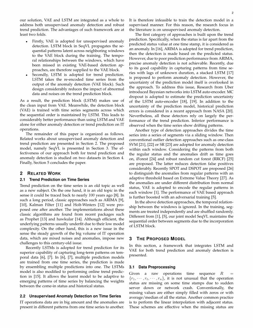
where w0 is the window size and yt is the predicted valuefrom the LSTM block. It basically measures the average errorthat the predicted yt differs from xt+1. In the evaluation, thefirst half of the time series is used to train the model, whilethe second half is used for evaluation. Since the anomaliesin the time series are annotated, they are removed from theseries when they are used for prediction evaluation. Theremoved time stamps are filled with the expected normalstatus. This is achieved with the same scheme used forfilling missing status during the pre-processing step. Aftercalculating the MSE of each time series, we plot them as boxplots to visualize the MSE score as well as the stability ofthe prediction models. The lower is MSE and the shorter isthe width of the box, and thus the higher is the predictionprecision.

Prophet ARIMA RM-LSTM LSTM SeqVL

Model

0

0.5

1

1.5

2

2.5

3

3.5

4

4.5

5

MSE

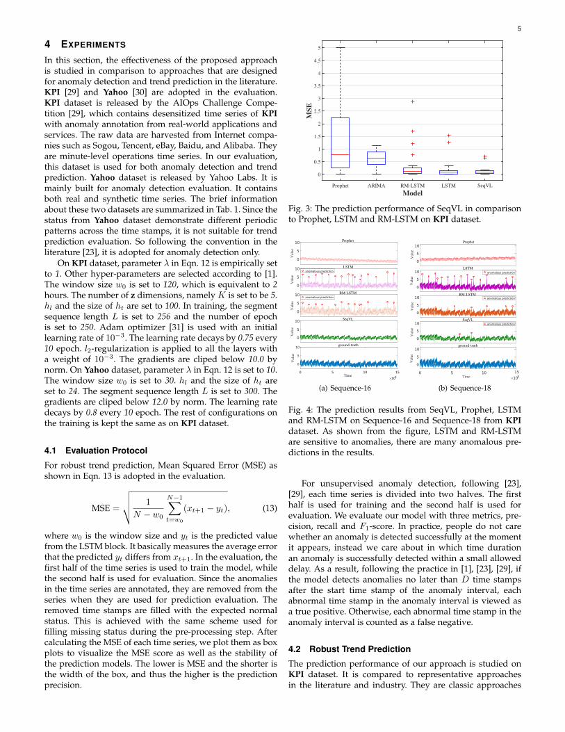
Fig. 3: The prediction performance of SeqVL in comparisonto Prophet, LSTM and RM-LSTM on KPI dataset.

0 5 10 15Time

×104

0

5

10

Val

ue

ground-truth

0

5

10

Val

ue

Prophet

0

5

10

Val

ue

SeqVL

0

5

10

Val

ue

LSTManomalous prediction

0

5

10V

alue

RM-LSTManomalous prediction

(a) Sequence-16

0 5 10Time

15 ×104

0

5

10

Val

ue

ground-truth

0

5

10

Val

ue

Prophet

0

5

10

Val

ue

LSTManomalous prediction

0

5

10

Val

ue

RM-LSTManomalous prediction

0

5

10

Val

ue

SeqVLanomalous prediction

(b) Sequence-18

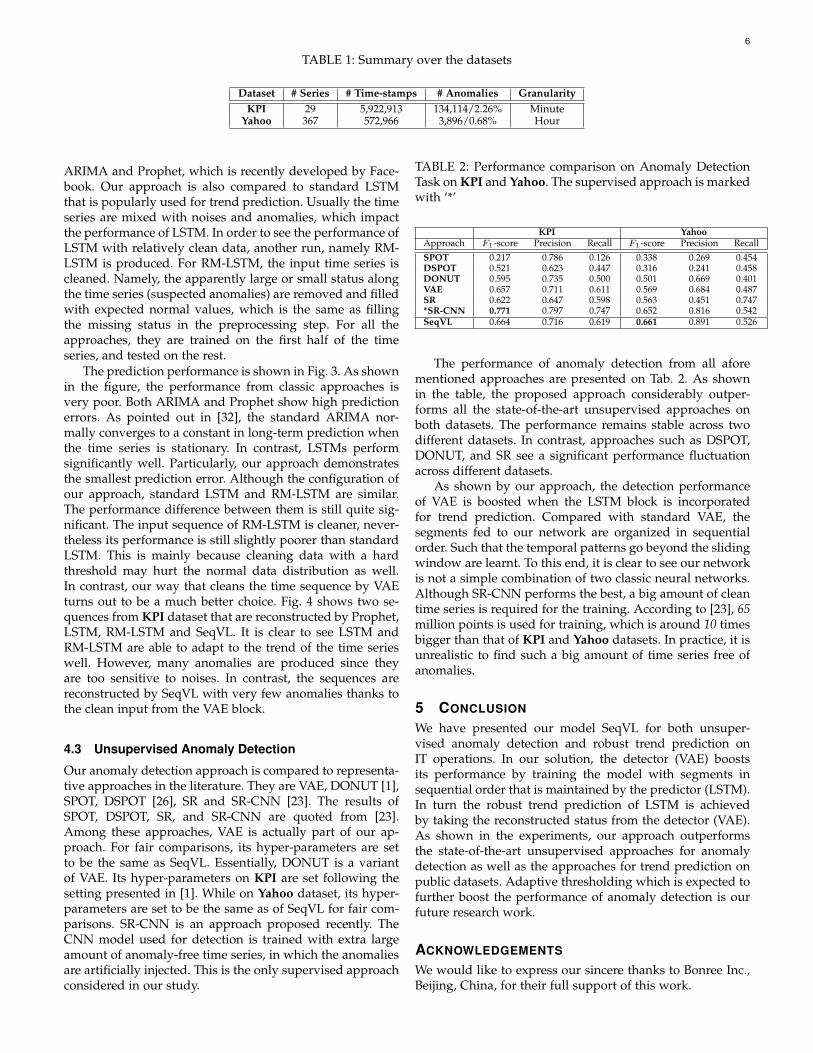
Fig. 4: The prediction results from SeqVL, Prophet, LSTMand RM-LSTM on Sequence-16 and Sequence-18 from KPIdataset. As shown from the figure, LSTM and RM-LSTMare sensitive to anomalies, there are many anomalous pre-dictions in the results.

For unsupervised anomaly detection, following [23],[29], each time series is divided into two halves. The firsthalf is used for training and the second half is used forevaluation. We evaluate our model with three metrics, pre-cision, recall and F1-score. In practice, people do not carewhether an anomaly is detected successfully at the momentit appears, instead we care about in which time durationan anomaly is successfully detected within a small alloweddelay. As a result, following the practice in [1], [23], [29], ifthe model detects anomalies no later than D time stampsafter the start time stamp of the anomaly interval, eachabnormal time stamp in the anomaly interval is viewed asa true positive. Otherwise, each abnormal time stamp in theanomaly interval is counted as a false negative.

4.2 Robust Trend Prediction

The prediction performance of our approach is studied onKPI dataset. It is compared to representative approachesin the literature and industry. They are classic approaches

6

TABLE 1: Summary over the datasets

Dataset # Series # Time-stamps # Anomalies GranularityKPI 29 5,922,913 134,114/2.26% Minute

Yahoo 367 572,966 3,896/0.68% Hour

ARIMA and Prophet, which is recently developed by Face-book. Our approach is also compared to standard LSTMthat is popularly used for trend prediction. Usually the timeseries are mixed with noises and anomalies, which impactthe performance of LSTM. In order to see the performance ofLSTM with relatively clean data, another run, namely RM-LSTM is produced. For RM-LSTM, the input time series iscleaned. Namely, the apparently large or small status alongthe time series (suspected anomalies) are removed and filledwith expected normal values, which is the same as fillingthe missing status in the preprocessing step. For all theapproaches, they are trained on the first half of the timeseries, and tested on the rest.

The prediction performance is shown in Fig. 3. As shownin the figure, the performance from classic approaches isvery poor. Both ARIMA and Prophet show high predictionerrors. As pointed out in [32], the standard ARIMA nor-mally converges to a constant in long-term prediction whenthe time series is stationary. In contrast, LSTMs performsignificantly well. Particularly, our approach demonstratesthe smallest prediction error. Although the configuration ofour approach, standard LSTM and RM-LSTM are similar.The performance difference between them is still quite sig-nificant. The input sequence of RM-LSTM is cleaner, never-theless its performance is still slightly poorer than standardLSTM. This is mainly because cleaning data with a hardthreshold may hurt the normal data distribution as well.In contrast, our way that cleans the time sequence by VAEturns out to be a much better choice. Fig. 4 shows two se-quences from KPI dataset that are reconstructed by Prophet,LSTM, RM-LSTM and SeqVL. It is clear to see LSTM andRM-LSTM are able to adapt to the trend of the time serieswell. However, many anomalies are produced since theyare too sensitive to noises. In contrast, the sequences arereconstructed by SeqVL with very few anomalies thanks tothe clean input from the VAE block.

4.3 Unsupervised Anomaly Detection

Our anomaly detection approach is compared to representa-tive approaches in the literature. They are VAE, DONUT [1],SPOT, DSPOT [26], SR and SR-CNN [23]. The results ofSPOT, DSPOT, SR, and SR-CNN are quoted from [23].Among these approaches, VAE is actually part of our ap-proach. For fair comparisons, its hyper-parameters are setto be the same as SeqVL. Essentially, DONUT is a variantof VAE. Its hyper-parameters on KPI are set following thesetting presented in [1]. While on Yahoo dataset, its hyper-parameters are set to be the same as of SeqVL for fair com-parisons. SR-CNN is an approach proposed recently. TheCNN model used for detection is trained with extra largeamount of anomaly-free time series, in which the anomaliesare artificially injected. This is the only supervised approachconsidered in our study.

TABLE 2: Performance comparison on Anomaly DetectionTask on KPI and Yahoo. The supervised approach is markedwith ‘*’

KPI YahooApproach F1-score Precision Recall F1-score Precision Recall

SPOT 0.217 0.786 0.126 0.338 0.269 0.454DSPOT 0.521 0.623 0.447 0.316 0.241 0.458DONUT 0.595 0.735 0.500 0.501 0.669 0.401VAE 0.657 0.711 0.611 0.569 0.684 0.487SR 0.622 0.647 0.598 0.563 0.451 0.747*SR-CNN 0.771 0.797 0.747 0.652 0.816 0.542SeqVL 0.664 0.716 0.619 0.661 0.891 0.526

The performance of anomaly detection from all aforementioned approaches are presented on Tab. 2. As shownin the table, the proposed approach considerably outper-forms all the state-of-the-art unsupervised approaches onboth datasets. The performance remains stable across twodifferent datasets. In contrast, approaches such as DSPOT,DONUT, and SR see a significant performance fluctuationacross different datasets.

As shown by our approach, the detection performanceof VAE is boosted when the LSTM block is incorporatedfor trend prediction. Compared with standard VAE, thesegments fed to our network are organized in sequentialorder. Such that the temporal patterns go beyond the slidingwindow are learnt. To this end, it is clear to see our networkis not a simple combination of two classic neural networks.Although SR-CNN performs the best, a big amount of cleantime series is required for the training. According to [23], 65million points is used for training, which is around 10 timesbigger than that of KPI and Yahoo datasets. In practice, it isunrealistic to find such a big amount of time series free ofanomalies.

5 CONCLUSION

We have presented our model SeqVL for both unsuper-vised anomaly detection and robust trend prediction onIT operations. In our solution, the detector (VAE) boostsits performance by training the model with segments insequential order that is maintained by the predictor (LSTM).In turn the robust trend prediction of LSTM is achievedby taking the reconstructed status from the detector (VAE).As shown in the experiments, our approach outperformsthe state-of-the-art unsupervised approaches for anomalydetection as well as the approaches for trend prediction onpublic datasets. Adaptive thresholding which is expected tofurther boost the performance of anomaly detection is ourfuture research work.

ACKNOWLEDGEMENTS

We would like to express our sincere thanks to Bonree Inc.,Beijing, China, for their full support of this work.

7

REFERENCES

[1] H. Xu, Y. Feng, J. Chen, Z. Wang, H. Qiao, W. Chen, N. Zhao, Z. Li,J. Bu, Z. Li, Y. Liu, Y. Zhao, and D. Pei, “Unsupervised AnomalyDetection via Variational Auto-Encoder for Seasonal KPIs in WebApplications,” in Proceeding of the International Conference on WorldWide Web, vol. 2, pp. 187–196, ACM, 2018.

[2] S. Hochreiter and S. Jurgen, “Long short-term memory,” NeuralComputation, vol. 9, pp. 1735–1780, nov 1997.

[3] R. J. Williams and D. Zipser, “A learning algorithm for continuallyrunning fully recurrent neural networks,” Neural Computation,vol. 1, pp. 270–280, Jun. 1989.

[4] D. P. Kingma and M. Welling, “Auto-encoding variational bayes,”CoRR, vol. abs/1312.6114, Dec. 2013.

[5] W. Chen, H. Xu, Z. Li, D. Pei, J. Chen, H. Qiao, Y. Feng, andZ. Wang, “Unsupervised anomaly detection for intricate KPIs viaadversarial training of vae,” in Proceedings of the IEEE InternationalConference on Computer Communications, pp. 1891–1899, IEEE, Apr.2019.

[6] J. Xue, F. Yan, R. Birke, L. Y. Chen, T. Scherer, and E. Smirni,“Practise: Robust prediction of data center time series,” in Proceed-ings of the IFIP/IEEE International Conference on Network and ServiceManagement, pp. 126–134, IEEE, Nov. 2015.

[7] A. Zameer, J. Arshad, A. Khan, and M. A. Z. Raja, “Intelligent androbust prediction of short term wind power using genetic pro-gramming based ensemble of neural networks,” Energy Conversionand Management, vol. 134, pp. 361–372, Feb. 2017.

[8] J. G. D. Gooijer and R. J. Hyndman, “25 years of time seriesforecasting,” International Journal of Forecasting, vol. 22, pp. 443–473, Jan. 2006.

[9] G. E. Box and G. M. Jenkins, Time series analysis: Forecasting andcontrol. Holden-Day, 1976.

[10] J. D. Salas, Applied modeling of hydrologic time series. Water Re-sources Publication, 1980.

[11] A. C. Harvey, Forecasting, structural time series models and the Kalmanfilter. Cambridge university press, 1990.

[12] P. Kalekar, “Time series forecasting using holt-winters exponentialsmoothing,” Kanwal Rekhi School of Information Technology, pp. 1–13, 2004.

[13] Facebook, “Prophet: Tool for producing high quality forecasts fortime series data that has multiple seasonality with linear or non-linear growth.,” 2017.

[14] Hawkular, “Hawkular for monitoring services: Metrics, alerting,inventory, application performance management.,” 2014.

[15] T. Guo, Z. Xu, X. Yao, H. Chen, K. Aberer, and K. Funaya, “Robustonline time series prediction with recurrent neural networks,” inProceedings of the IEEE International Conference on Data Science andAdvanced Analytics, pp. 816–825, IEEE, Oct. 2016.

[16] A. H. Yaacob, I. K. Tan, S. F. Chien, and H. K. Tan, “Arima basednetwork anomaly detection,” in Proceedings of the IEEE InternationalConference on Communication Software and Networks, pp. 205–209,IEEE, 2010.

[17] P. Malhotra, L. Vig, G. Shroff, and P. Agarwal, “Long short termmemory networks for anomaly detection in time series,” in Pro-ceedings of the European Symposium on Artificial Neural Networks,Computational Intelligence and Machine Learning, pp. 89–94, 2015.

[18] N. Laptev, J. Yosinski, L. E. Li, and S. Smyl, “Time-series extremeevent forecasting with neural networks at uber,” in Proceedingsof the International Conference on Machine Learning - Time SeriesWorkshop, vol. 13, pp. 1–5, Jan. 2017.

[19] L. Zhu and N. Laptev, “Deep and confident prediction for timeseries at uber,” in Proceedings of the IEEE International Conference onData Mining Workshops, vol. 2017-Novem, pp. 103–110, IEEE, Nov.2017.

[20] K. Hundman, V. Constantinou, C. Laporte, I. Colwell, andT. Soderstrom, “Detecting spacecraft anomalies using lstms andnonparametric dynamic thresholding,” in Proceedings of the ACMSIGKDD International Conference on Knowledge Discovery and DataMining, pp. 387–395, ACM, 2018.

[21] C. Campbell and K. P. Bennett, “A linear programming approachto novelty detection,” in Advances in Neural Information ProcessingSystems, 2001.

[22] B. Scholkopf, R. Williamson, A. Smola, J. Shawe-Taylor, and J. Pi-att, “Support vector method for novelty detection,” in Advances inNeural Information Processing Systems, pp. 582–588, 2000.

[23] H. Ren, Q. Zhang, B. Xu, Y. Wang, C. Yi, C. Huang, X. Kou, T. Xing,M. Yang, and J. Tong, “Time-series anomaly detection serviceat microsoft,” in Proceedings of the ACM SIGKDD International

Conference on Knowledge Discovery and Data Mining, pp. 3009–3017,ACM, Jun. 2019.

[24] Z. Ding and M. Fei, “An anomaly detection approach basedon isolation forest algorithm for streaming data using slidingwindow,” IFAC Proceedings Volumes, vol. 46, pp. 12–17, Jan. 2013.

[25] S. Guha, N. Mishra, G. Roy, and O. Schrijvers, “Robust random cutforest based anomaly detection on streams,” in Proceedings of theInternational Conference on Machine Learning, vol. 48, pp. 2712–2721,2016.

[26] A. Siffer, P. A. Fouque, A. Termier, and C. Largouet, “Anomalydetection in streams with extreme value theory,” in Proceedings ofthe ACM SIGKDD International Conference on Knowledge Discoveryand Data Mining, vol. Part F1296, pp. 1067–1075, ACM Press, 2017.

[27] L. de Haan and A. Ferreira, Extreme Value Theory. Springer Seriesin Operations Research and Financial Engineering, Springer NewYork, 2006.

[28] J. An and S. Cho, “Variational autoencoder based anomaly detec-tion using reconstruction probability,” Special Lecture on IE, Feb.2015.

[29] AIOpsChallenge, “KPI anomaly detection competition,” 2017.[30] YahooLabs, “S5 - a labeled anomaly detection dataset, version 1.0,”

2015.[31] D. P. Kingma and J. Ba, “Adam: A method for stochastic optimiza-

tion,” CoRR, vol. abs/1412.6980, Dec. 2014.[32] R. J. Hyndman and G. Athanasopoulos, Forecasting: principles and

practice. OTexts, 2018.