Embed Size (px)
Citation preview
1
Semblance analysis to assess GPR data from a five-year forensic study of 1
simulated clandestine graves 2
3
Adam D. Booth1*, Jamie K. Pringle2 4
1. [email protected]; Department of Earth Science and Engineering, Imperial 5
College London, South Kensington Campus, London, SW7 2AZ, UK 6
2. [email protected]; School of Physical and Geographical Sciences, Keele 7
University, Keele, Staffordshire ST5 5BG, UK 8
9
Abstract 10
11
Ground penetrating radar (GPR) surveys have proven useful for locating clandestine 12
graves in a number of forensic searches. There has been extensive research into 13
the geophysical monitoring of simulated clandestine graves in different burial 14
scenarios and ground conditions. Whilst these studies have been used to suggest 15
optimum dominant radar frequencies, the data themselves have not been 16
quantitatively analysed to-date. This study uses a common-offset configuration of 17
semblance analysis, both to characterise velocity trends from GPR diffraction 18
hyperbolae and, since the magnitude of a semblance response is proportional to 19
signal-to-noise ratio, to quantify the strength of a forensic GPR response. 2D GPR 20
profiles were acquired over a simulated clandestine burial, with a wrapped-pig 21
cadaver monitored at three-month intervals between 2008-2013 with GPR antennas 22
2
of three different centre-frequencies (110, 225 and 450 MHz). The GPR response to 1
the cadaver was a strong diffraction hyperbola. Results show, in contrast to 2
resistivity surveys, that semblance analysis show little sensitivity to changes 3
attributable to decomposition, and only a subtle influence of seasonality: velocity 4
increases (0.01-0.02 m/ns) were observed in summer, associated with a decrease 5
(5-10%) in peak semblance magnitude, SM, and potentially in the reflectivity of the 6
grave. The lowest-frequency antennas consistently gave the highest signal-to-noise 7
ratio although the grave was nonetheless detectable by all frequencies trialled. This 8
therefore suggests forensic radar surveys should be undertaken without regard to 9
seasonality. Whilst GPR analysis cannot currently provide a quantitative diagnostic 10
proxy for time-since-burial, the consistency of responses suggests that graves will 11
remain detectable beyond the five years shown here. 12
13
14
15
16
17
18
19
20
21
22
3
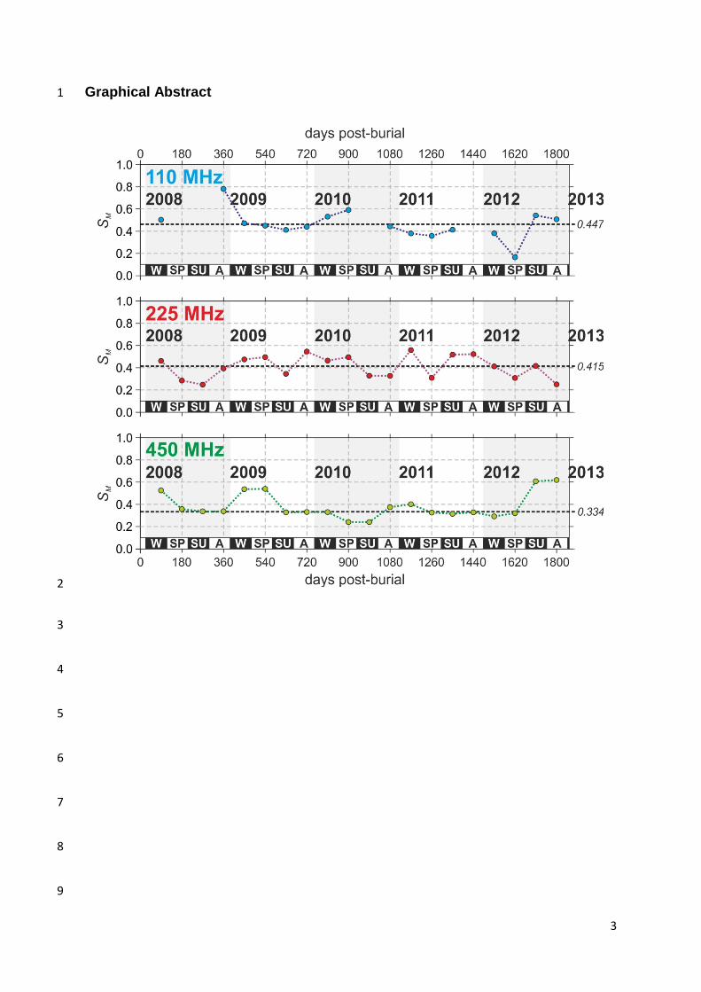
Graphical Abstract 1
2
3
4
5
6
7
8
9
4
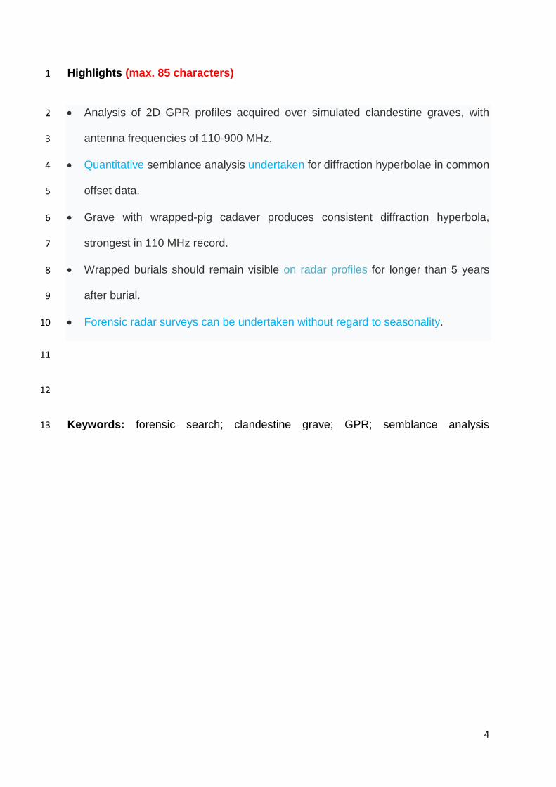
Highlights (max. 85 characters) 1
• Analysis of 2D GPR profiles acquired over simulated clandestine graves, with 2
antenna frequencies of 110-900 MHz. 3
• Quantitative semblance analysis undertaken for diffraction hyperbolae in common 4
offset data. 5
• Grave with wrapped-pig cadaver produces consistent diffraction hyperbola, 6
strongest in 110 MHz record. 7
• Wrapped burials should remain visible on radar profiles for longer than 5 years 8
after burial. 9
• Forensic radar surveys can be undertaken without regard to seasonality. 10
11
12
Keywords: forensic search; clandestine grave; GPR; semblance analysis13
5
1. Introduction 1
2
There are numerous and varied methods employed by forensic search teams to 3
detect the clandestine burial of murder victims (Pringle et al., 2012a; Parker et al., 4
2010). Current best practice suggests a phased approach, which moves from large-5
scale remote sensing methods (Kalacska et al., 2009) through to initial ground 6
reconnaissance (Ruffell and McKinley, 2014) and control studies before full searches 7
are initiated (Harrison and Donnelly, 2009; Larsen et al., 2011). These full searches 8
have themselves involved a variety of methods including, for example, forensic 9
geomorphology (Ruffell and McKinley, 2014), forensic botany (Aquila et al., 2014) 10
and entomology (Amendt et al., 2007), scent-trained search dogs (Lasseter et al., 11
2003), physical probing (Ruffell, 2005a), thanatochemistry (Vass, 2012) and near-12
surface geophysics (see e.g. France et al., 1992; Powell, 2004; Nobes, 2000; 13
Cheetham, 2005; Pringle and Jervis, 2009). 14
15
Near-surface geophysics appeals in forensic searches principally because of survey 16
efficiency and non-invasiveness. Ground penetrating radar is arguably the most 17
commonly used near-surface geophysical technique for clandestine grave detection 18
(see e.g. Mellet, 1992; Calkin et al., 1995; Davenport, 2001; Ruffell, 2005b; Schultz, 19
2007; Billinger, 2009; Novo et al., 2011; Ruffell et al., 2014), and Nobes (2000) 20
deploys the technique alongside electromagnetic prospection methods. Forensic 21
burials differ strongly from historical and/or archaeological graves (e.g. Fiedler et al., 22
2009; Hansen et al., 2014). Archaeological examples can be difficult, though not 23
impossible, to detect due to limited skeletal remains and processes of soil 24
6
compaction (Vaughan, 1986); however, archaeological graves can be associated 1
with monumental and/or ceremonial features, which are more readily detected. 2
While the clandestine burial lacks any monumental features, organic remains are 3
often present and the burial is typically shallow. As such, while archaeological 4
survey methodologies may be replicated in forensic searches, the style and 5
composition of the grave and its contents vary between the two settings. 6
7
Several recent GPR control studies use animal remains as a proxy for human 8
remains in constructed graves, which are then repeatedly surveyed over extensive 9
time periods (see e.g. France et al., 1992; Buck, 2003; Schultz et al., 2006; Schultz, 10
2007; Pringle et al., 2008; Schultz, 2008; Schultz and Martin, 2011; Pringle et al., 11
2012b; Schultz and Martin, 2012). These studies aim to determine optimal antenna 12
centre-frequencies for numerous variables, including different time periods post-13
burial, varied burial styles, different soil types and local depositional environments. 14
However, the assessment of GPR results has largely been visual, qualitative and/or 15
subjective (Pringle et al., 2012b). This contrasts with a recent example of resistivity 16
analysis, in which an objective and quantitative approach to characterising electrical 17
responses was developed (Jervis and Pringle, 2014). 18
19
In this study, we develop a semblance-based method to quantify the assessment of 20
a time-lapse archive of GPR observations from a simulated clandestine burial site. 21
Semblance analysis, familiar for applications to data in the common midpoint (CMP) 22
domain, is novelly? adapted to 2D profiles of common offset GPR data. We 23
demonstrate that the peak magnitude of semblance response can be used as an 24
7
indicator of signal-to-noise ratio, which in turn describes the underlying target 1
reflectivity. We then consider the implications of semblance responses for the 2
interpretation of real data. 3
4
2. Methods 5
Here, we describe the existing archive of pre-recorded GPR data, and describe the 6
use of semblance analysis as a quantitative assessment tool. 7
2.1. Study background 8
This study focuses on the GPR archive of time-lapse geophysical observations 9
acquired at a test site, where buried pig cadavers were used as a proxy for 10
clandestine graves (Pringle et al. 2012b). The site is former garden land in the 11
campus of Keele University (Staffordshire, UK) and is deemed typical of a semi-rural 12
environment in the UK. The site vegetation is grassy with small deciduous trees on 13
three sides. The soil at the site is predominantly sandy loam, above the local water 14
table with ~0.31 average fractional soil moisture content recorded over the first two 15
years of monitoring (Jervis et al. 2009), with fragments of shallow sandstone bedrock 16
present at depths below ground level (bgl) exceeding 0.5 m and bedrock itself at 17
~2.5 m bgl. Three graves were dug at an interval of approximately 4 m, to a depth of 18
0.5 m bgl (representing a clandestine grave construction halted when encountering 19
hard rock fragments). Pig cadavers weighing approximately 80 kg were placed in 20
two graves before backfilling; the third grave was left empty and backfilled as a 21
control. One pig cadaver was left naked (termed the ‘naked-pig grave’) and the 22
second was wrapped in a porous tarpaulin (termed the ‘wrapped-pig grave’) (see 23
8
Jervis et al., 2009), to simulate the two commonest scenarios of murder victims (see 1
Hunter & Cox, 2005). The study site remained dedicated as such throughout the 2
study period and was subject to no change for its duration excepting natural 3
processes. Extended discussion of the construction of the test site, and of the full 4
suite of geophysical archives, is given in Jervis et al. (2009), Pringle et al. (2012b) 5
and Jervis and Pringle (2014). In this analysis, we consider only the GPR profiles 6
acquired over the wrapped-pig grave. 7
8
2.3 GPR survey data collection and basic processing 9
GPR profile positions were permanently marked in the field by non-conductive plastic 10
pegs at the respective start/end positions and survey tapes allowed the accurate 11
collection of quarterly repeat surveys, using the respective centre frequency sample 12
spacings listed in Table 1, over the five year monitoring period. Sensors&Software 13
PulseEKKO1000™ equipment was used to collect 2D common offset (CO) profiles, 14
using antenna sets of 110 MHz, 225 MHz, and 450 MHz centre-frequency 15
(acquisition parameters listed in Table 1). Throughout the monitoring period, vertical 16
sample stacking (repeats) was set to 32 for consistency. Data were processed in 17
Sandmeier ReflexW© version? software, using sequential ‘dewow’ and Ormsby 18
bandpass filters, static corrections to align time-zero within each trace, and a gain 19
function based on the energy decay curve within each trace (Table 2). No form of 20
migration is applied since this would collapse the diffraction hyperbolae which are 21
the key focus of our analysis. Additionally, there is no topographic variation across 22
the site hence static corrections are constant for each profile. 23
24
9
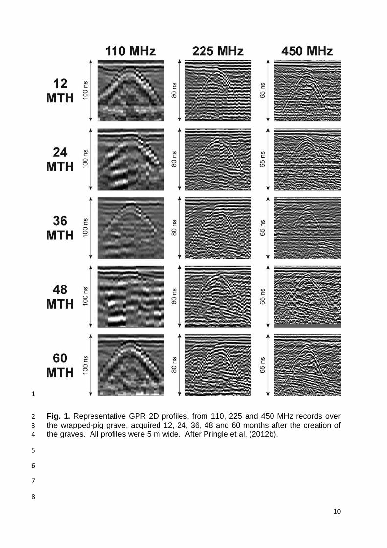
Representative time-lapse profiles acquired over the wrapped-pig grave are shown 1
in Figure 1, the full suite of which is later supplied to semblance analysis for 2
additional characterisation. The response to the wrapped-pig burial was a diffraction 3
hyperbola, typically prominent throughout the survey period for all antenna 4
frequencies acquired. 5
6
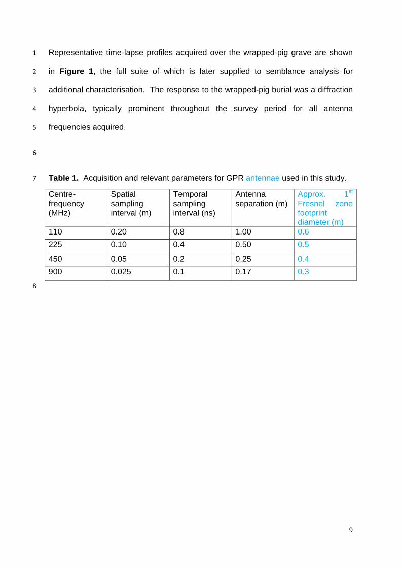
Table 1. Acquisition and relevant parameters for GPR antennae used in this study. 7
Centre-frequency (MHz)
Spatial sampling interval (m)
Temporal sampling interval (ns)
Antenna separation (m)
Approx. 1st Fresnel zone footprint diameter (m)
110 0.20 0.8 1.00 0.6 225 0.10 0.4 0.50 0.5
450 0.05 0.2 0.25 0.4 900 0.025 0.1 0.17 0.3
8
10
1
Fig. 1. Representative GPR 2D profiles, from 110, 225 and 450 MHz records over 2 the wrapped-pig grave, acquired 12, 24, 36, 48 and 60 months after the creation of 3 the graves. All profiles were 5 m wide. After Pringle et al. (2012b). 4
5
6
7
8
11
2.4 Semblance as a measure of data quality 1 2 Semblance is commonly applied in seismic and GPR velocity analysis routines (see, 3
e.g., Yilmaz, 2001; Porsani et al., 2006; Fomel and Landa, 2014), which seek to 4
derive a subsurface velocity distribution from travel-time relationships in a dataset. 5
Typically, semblance analysis is applied to reflection hyperbola in the common 6
midpoint (CMP) domain, where the travel-time, t(x), of energy reflected from the 7
horizontal base of homogeneous, isotropic, overburden is approximated by the 8
‘normal moveout’ (NMO) equation: 9
t(x)2 = t02 + (x2 / VST2), (Eq. 1) 10
where x is the source-receiver offset, t0 is the travel-time to that base at x = 0, and 11
VST is termed ‘stacking velocity’, a near-offset approximation to root-mean-square 12
velocity VRMS. For the case of a single overburden layer, VRMS is equivalent to 13
interval velocity, VINT, the propagation velocity within any one interval of the 14
subsurface. The semblance statistic then provides a measure of the coherency of 15
energy along trial trajectories defined by the substitution of trial pairs of VST and t0 16
into Equation (1). 17
18
However, the data considered in this study were profiles of common offset (CO) data 19
and the responses to be analysed in semblance analysis were diffraction, rather than 20
reflection, hyperbolae. As such, the NMO equation was reconfigured for diffraction 21
trajectories in the CO profile, such that travel-time, t(x), was approximated as: 22
t(x)2 = t(x0)2 + (4(x-x0)2/vST2), (Eq. 2) 23
12
with x redefined as the position along a profile, x0 as the surface position vertically 1
above the diffracting target and t(x0) as the travel-time to the target when antennas 2
are positioned at x0 (see Ristic et al., 2009). By substituting trial x0, t(x0) and VST 3
values into Equation (2), semblance is therefore measured along trajectories 4
corresponding to diffraction hyperbolae in the GPR profile. 5
6
In addition to the objective definition of a subsurface velocity distribution from 7
diffraction hyperbolae (as opposed to subjective curve-fitting), the semblance 8
statistic could also provide an objective measure of data quality in terms of velocity 9
resolution and signal-to-noise ratio (SNR). Assuming that the only changes within a 10
time-lapse dataset are related to subsurface processes, and not environmental ones 11
(e.g., ambient noise level), the changing semblance response could provide a proxy 12
for the evolving reflectivity of the target and/or its detectability against background 13
noise levels. 14
15
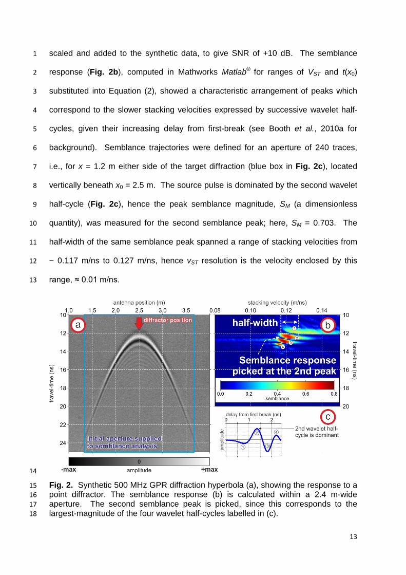
The relationship between signal-to-noise ratio and semblance-derived parameters 16
was explored for synthetic GPR data (Fig. 2a), simulated using GprMax (see 17
Giannopoulos, 2005). Specifically, synthetic data were used to investigate how 18
variations in SNR are manifested in the peak magnitude and the velocity resolution 19
expressed by a semblance response. The simulation represented the GPR 20
response over a point diffractor, located at a depth of 0.7 m within a homogeneous 21
layer of constant interval velocity of 0.12 m/ns; the GPR pulse was approximated by 22
a 500 MHz Ricker wavelet, transmitted from a monostatic antenna with a spatial 23
sampling interval of 0.01 m. Normally-distributed random noise amplitudes were 24
13
scaled and added to the synthetic data, to give SNR of +10 dB. The semblance 1
response (Fig. 2b), computed in Mathworks Matlab® for ranges of VST and t(x0) 2
substituted into Equation (2), showed a characteristic arrangement of peaks which 3
correspond to the slower stacking velocities expressed by successive wavelet half-4
cycles, given their increasing delay from first-break (see Booth et al., 2010a for 5
background). Semblance trajectories were defined for an aperture of 240 traces, 6
i.e., for x = 1.2 m either side of the target diffraction (blue box in Fig. 2c), located 7
vertically beneath x0 = 2.5 m. The source pulse is dominated by the second wavelet 8
half-cycle (Fig. 2c), hence the peak semblance magnitude, SM (a dimensionless 9
quantity), was measured for the second semblance peak; here, SM = 0.703. The 10
half-width of the same semblance peak spanned a range of stacking velocities from 11
~ 0.117 m/ns to 0.127 m/ns, hence vST resolution is the velocity enclosed by this 12
range, ≈ 0.01 m/ns. 13
14
Fig. 2. Synthetic 500 MHz GPR diffraction hyperbola (a), showing the response to a 15 point diffractor. The semblance response (b) is calculated within a 2.4 m-wide 16 aperture. The second semblance peak is picked, since this corresponds to the 17 largest-magnitude of the four wavelet half-cycles labelled in (c). 18
14
1
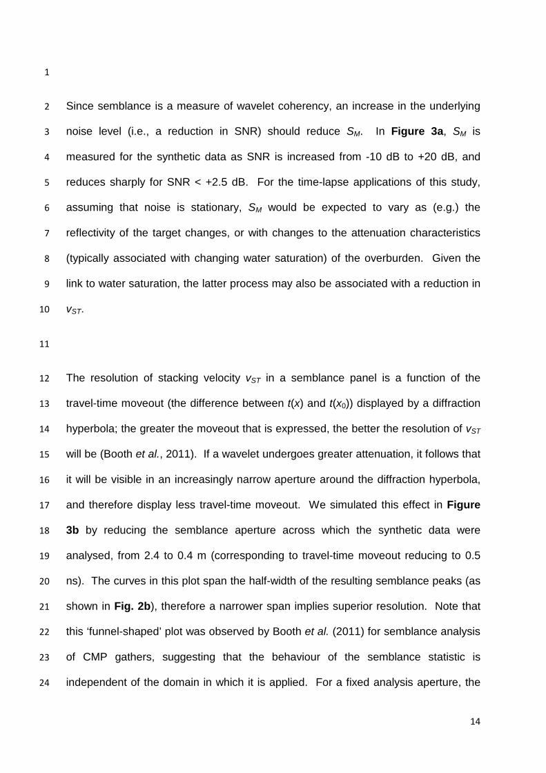
Since semblance is a measure of wavelet coherency, an increase in the underlying 2
noise level (i.e., a reduction in SNR) should reduce SM. In Figure 3a, SM is 3
measured for the synthetic data as SNR is increased from -10 dB to +20 dB, and 4
reduces sharply for SNR < +2.5 dB. For the time-lapse applications of this study, 5
assuming that noise is stationary, SM would be expected to vary as (e.g.) the 6
reflectivity of the target changes, or with changes to the attenuation characteristics 7
(typically associated with changing water saturation) of the overburden. Given the 8
link to water saturation, the latter process may also be associated with a reduction in 9
vST. 10
11
The resolution of stacking velocity vST in a semblance panel is a function of the 12
travel-time moveout (the difference between t(x) and t(x0)) displayed by a diffraction 13
hyperbola; the greater the moveout that is expressed, the better the resolution of vST 14
will be (Booth et al., 2011). If a wavelet undergoes greater attenuation, it follows that 15
it will be visible in an increasingly narrow aperture around the diffraction hyperbola, 16
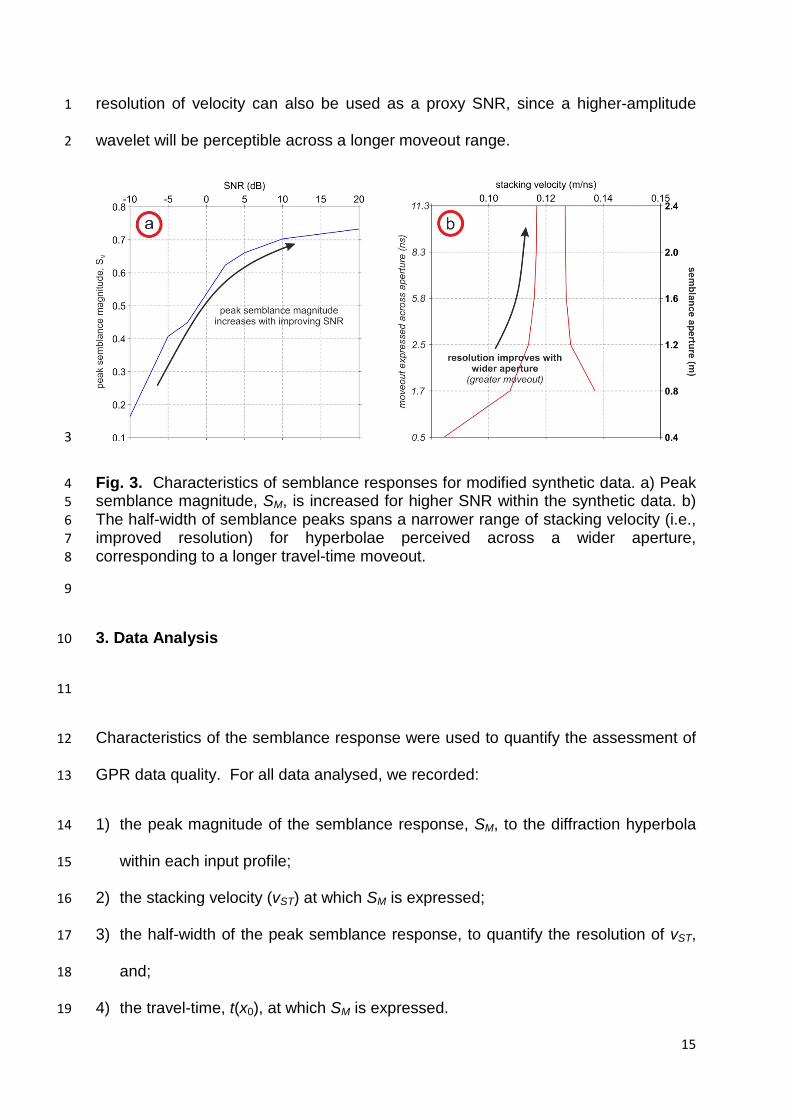
and therefore display less travel-time moveout. We simulated this effect in Figure 17
3b by reducing the semblance aperture across which the synthetic data were 18
analysed, from 2.4 to 0.4 m (corresponding to travel-time moveout reducing to 0.5 19
ns). The curves in this plot span the half-width of the resulting semblance peaks (as 20
shown in Fig. 2b), therefore a narrower span implies superior resolution. Note that 21
this ‘funnel-shaped’ plot was observed by Booth et al. (2011) for semblance analysis 22
of CMP gathers, suggesting that the behaviour of the semblance statistic is 23
independent of the domain in which it is applied. For a fixed analysis aperture, the 24
15
resolution of velocity can also be used as a proxy SNR, since a higher-amplitude 1
wavelet will be perceptible across a longer moveout range. 2
3
Fig. 3. Characteristics of semblance responses for modified synthetic data. a) Peak 4 semblance magnitude, SM, is increased for higher SNR within the synthetic data. b) 5 The half-width of semblance peaks spans a narrower range of stacking velocity (i.e., 6 improved resolution) for hyperbolae perceived across a wider aperture, 7 corresponding to a longer travel-time moveout. 8
9
3. Data Analysis 10
11
Characteristics of the semblance response were used to quantify the assessment of 12
GPR data quality. For all data analysed, we recorded: 13
1) the peak magnitude of the semblance response, SM, to the diffraction hyperbola 14
within each input profile; 15
2) the stacking velocity (vST) at which SM is expressed; 16
3) the half-width of the peak semblance response, to quantify the resolution of vST, 17
and; 18
4) the travel-time, t(x0), at which SM is expressed. 19
16
While quantifying the assessment of GPR data quality, any systematic variation in 1
these quantities could also be diagnostic of some decompositional process acting on 2
the burials, or a change in the local overburden. 3
4
All GPR profiles were exported from ReflexW© processing software into Mathworks 5
Matlab® for semblance analysis, and continuous time series of semblance 6
characteristics could be derived for the five-year study period. All semblance 7
analyses considered a range of trial stacking velocities from 0.05-0.12 m/ns, in 8
increments of 0.0001 m/ns. The reference position, x0, was taken in all cases to be 9
2.4 m (the position of the trace in which the apex of the diffraction hyperbola was 10
perceived), and t(x0) spanned a range from 0-30 ns in increments equal to the 11
temporal sampling interval of the input data (see Table 1). The semblance analysis 12
window also spanned an interval equivalent to one temporal sample, to give the 13
highest-resolution semblance response (see Booth et al., 2011 for background). The 14
analysis aperture was fixed at 4 m in all cases, consistent with the widest range of 15
traces over which the diffraction hyperbola could be perceived. 16
17
18
17
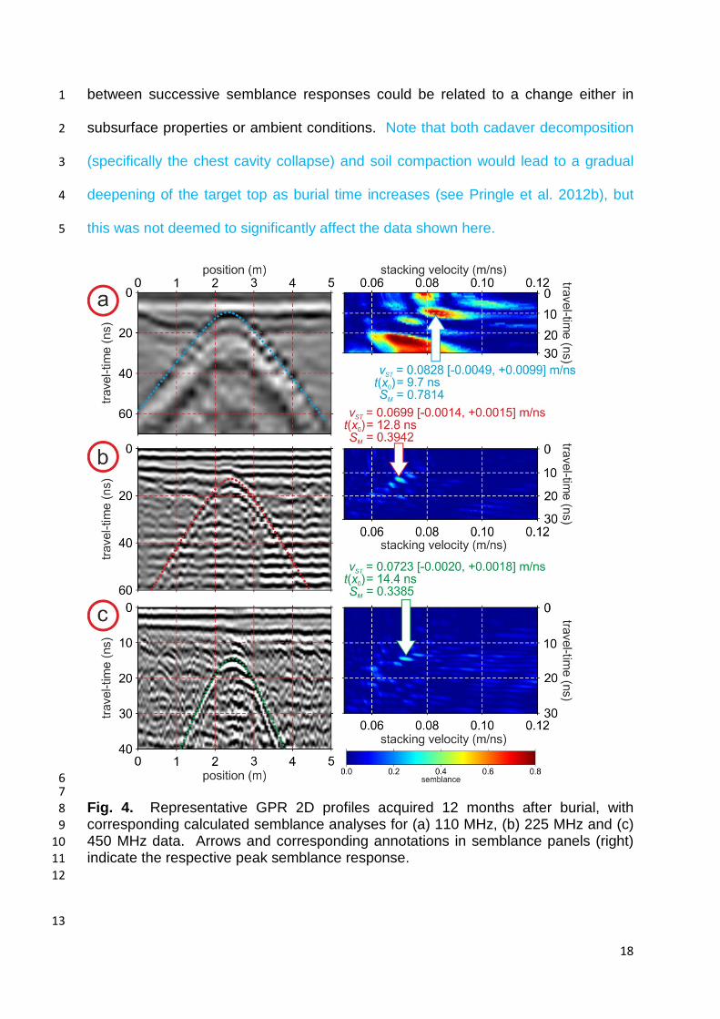
4. Results 1 2
Figure 4 shows diffraction hyperbolae in GPR 2D profiles, and their corresponding 3
semblance responses. This illustrative example, shown here for profiles acquired 4
over the graves one year after their creation (the ‘12 MTH’ set of profiles in Fig. 1), 5
was repeated for all profiles in the study. The hyperbolic curves which overlie the 6
profiles were defined by substituting the VST and t(x0) pair expressed at the peak 7
semblance response (as annotated in Fig. 4) into Equation (2). The 110 MHz 8
response showed the highest peak semblance (> double that of the other 9
diffractions) but, consistent with its lower frequency (Booth et al., 2011), the poorest 10
velocity resolution. 11
12
Although the 2D profiles were acquired over the same target, each hyperbola 13
expressed a different stacking velocity and travel-time. This effect was partly 14
attributable to effects of target geometry (i.e., the size of the target scattered different 15
components of each frequency-limited wavelet), but also to the incorrect assumption 16
in Equation (2) that there is zero offset between antennas (i.e., a monostatic GPR 17
system). No correction was made for this since it would require a priori knowledge of 18
the RMS velocity, but the necessary travel-time corrections could be included into 19
the semblance analysis if required. Nevertheless, the semblance parameters we 20
obtained should not be interpreted in terms of absolute subsurface properties (e.g., 21
dielectric permittivity, or target radius; see Shihab and Al-Nuaimy, 2005; Ristic et al., 22
2009 for background); instead, they were simply the quantities that the hyperbolae 23
express. However, since the geometry of the acquisition surveys never changed 24
throughout the survey period due to the permanent marked lines, relative differences 25
18
between successive semblance responses could be related to a change either in 1
subsurface properties or ambient conditions. Note that both cadaver decomposition 2
(specifically the chest cavity collapse) and soil compaction would lead to a gradual 3
deepening of the target top as burial time increases (see Pringle et al. 2012b), but 4
this was not deemed to significantly affect the data shown here. 5
6 7 Fig. 4. Representative GPR 2D profiles acquired 12 months after burial, with 8 corresponding calculated semblance analyses for (a) 110 MHz, (b) 225 MHz and (c) 9 450 MHz data. Arrows and corresponding annotations in semblance panels (right) 10 indicate the respective peak semblance response. 11 12
13
19
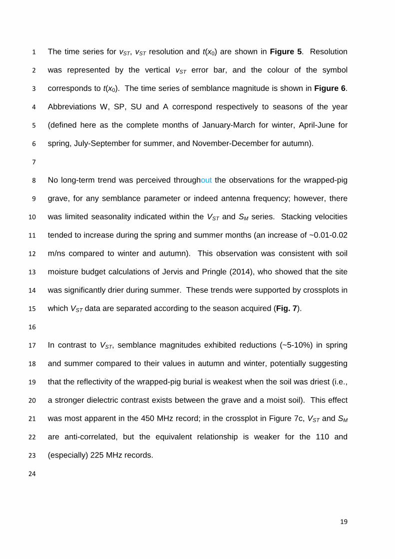
The time series for vST, vST resolution and t(x0) are shown in Figure 5. Resolution 1
was represented by the vertical vST error bar, and the colour of the symbol 2
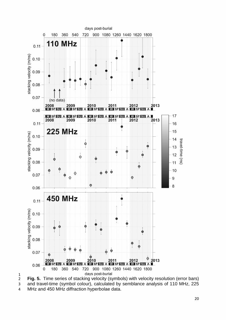
corresponds to t(x0). The time series of semblance magnitude is shown in Figure 6. 3
Abbreviations W, SP, SU and A correspond respectively to seasons of the year 4
(defined here as the complete months of January-March for winter, April-June for 5
spring, July-September for summer, and November-December for autumn). 6
7
No long-term trend was perceived throughout the observations for the wrapped-pig 8
grave, for any semblance parameter or indeed antenna frequency; however, there 9
was limited seasonality indicated within the VST and SM series. Stacking velocities 10
tended to increase during the spring and summer months (an increase of ~0.01-0.02 11
m/ns compared to winter and autumn). This observation was consistent with soil 12
moisture budget calculations of Jervis and Pringle (2014), who showed that the site 13
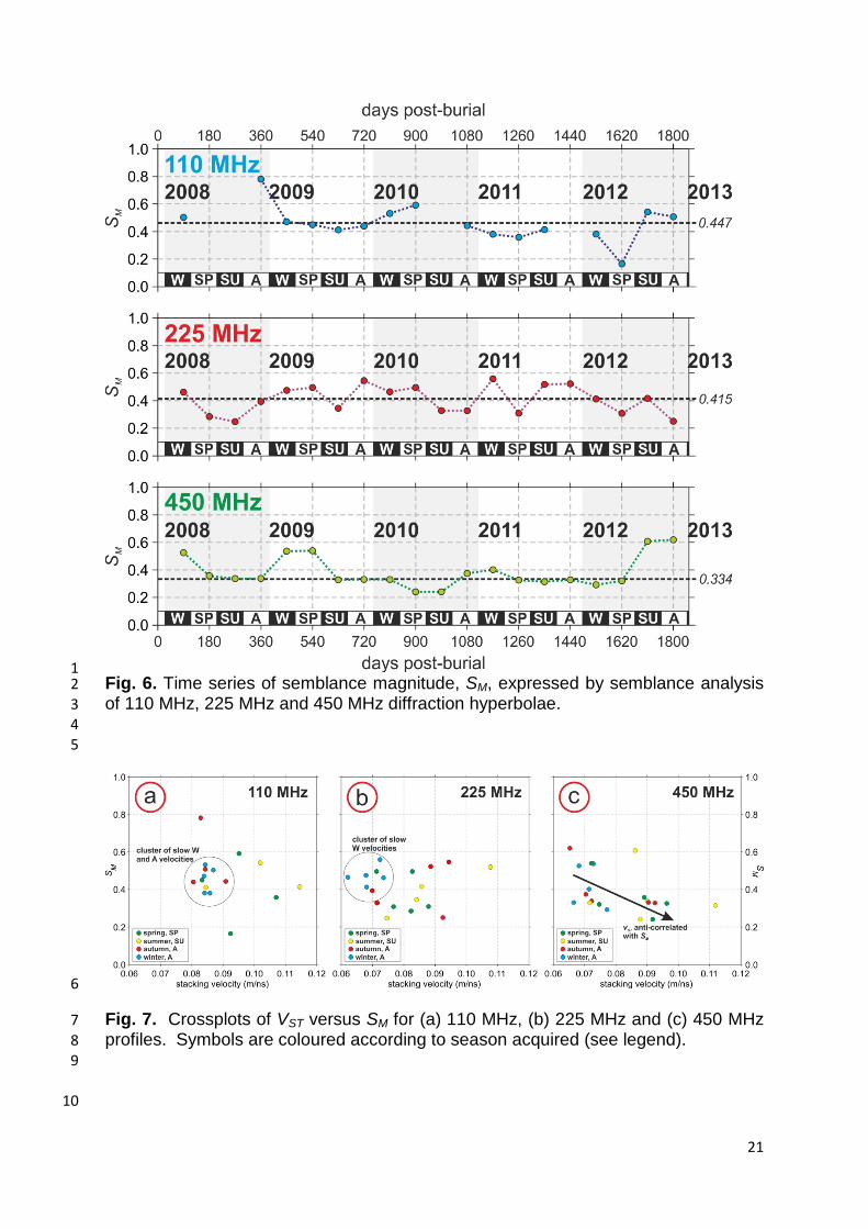
was significantly drier during summer. These trends were supported by crossplots in 14
which VST data are separated according to the season acquired (Fig. 7). 15
16
In contrast to VST, semblance magnitudes exhibited reductions (~5-10%) in spring 17
and summer compared to their values in autumn and winter, potentially suggesting 18
that the reflectivity of the wrapped-pig burial is weakest when the soil was driest (i.e., 19
a stronger dielectric contrast exists between the grave and a moist soil). This effect 20
was most apparent in the 450 MHz record; in the crossplot in Figure 7c, VST and SM 21
are anti-correlated, but the equivalent relationship is weaker for the 110 and 22
(especially) 225 MHz records. 23
24
20
1 Fig. 5. Time series of stacking velocity (symbols) with velocity resolution (error bars) 2 and travel-time (symbol colour), calculated by semblance analysis of 110 MHz, 225 3 MHz and 450 MHz diffraction hyperbolae data. 4
21
1 Fig. 6. Time series of semblance magnitude, SM, expressed by semblance analysis 2 of 110 MHz, 225 MHz and 450 MHz diffraction hyperbolae. 3 4 5
6
Fig. 7. Crossplots of VST versus SM for (a) 110 MHz, (b) 225 MHz and (c) 450 MHz 7 profiles. Symbols are coloured according to season acquired (see legend). 8 9
10
22
Interestingly, even with the pig cadaver gradually decomposing and with some 1
overlying soil compaction occurring over the five year study period, the combined VST 2
and t(x0) quantities consistently estimated the depth of the burial as 0.50 m ± 0.07 m, 3
suggesting that geometric changes were not significant (see Shibab and Al-Nuaimy, 4
2005). The 1st Fresnel zone footprints (see Cassidy et al. 2011 for background) of 5
the different radar centre frequency antennae (Table 1) were also not found to be 6
problematic in detecting the target burial. 7
8 9
23
5. Discussion 1
2
In their study of simulated grave sites, Jervis and Pringle (2014) quantified the 3
resistivity response of wrapped- and naked-pig burials over a five year monitoring 4
period, and cautioned that seasonal variations may make grave-related anomaly(s) 5
undetectable at certain times of the year, in particular the summer. Although limited 6
primarily to the study of the wrapped-pig grave, the quantitative semblance analyses 7
we have performed show, by contrast, no evidence of a systematic evolution of GPR 8
properties over the course of the survey, and only a small seasonal control on the 9
responses. GPR methods are therefore unlikely to be readily sensitive to changes in 10
the condition of a burial, and are instead more directly influenced by the 11
environmental state (e.g., water content) of the host soil material. This insensitivity 12
likely impedes the forensic application of GPR semblance analysis to date a burial. 13
However, by contrast with resistivity methods (Jervis and Pringle, 2014), there was 14
also no time of the year which could be described as obstructive to GPR methods; 15
hence a forensic search team could expect similar results from the GPR survey 16
regardless of when the survey was conducted. 17
18
The highest semblance magnitudes were typically observed for the 110 MHz data 19
(their mean SM was 13%, and 20%, higher than those of the 225 MHz and 450 MHz 20
series, respectively), presumably because SNR in the low frequency dataset was 21
higher given the reduced signal attenuation. While antenna frequencies should be 22
chosen on a site and/or target-specific basis, we suggest that semblance analysis 23
offers no practical limitation on the lowest recommendable frequency, an observation 24
made by other researchers (e.g. Schultz and Martin, 2011; Pringle et al. 2012b). 25
24
1
Semblance analysis was a promising means of quantifying the assessment of GPR 2
data profiles, but only where targets (such as wrapped-pig burials) were expressed 3
as diffraction hyperbolae. The method would be unsuitable for assessing data in 4
which targets do not present prominent diffractions, including the majority of the 2D 5
profiles acquired over the naked pigs (Pringle et al. 2012b). However, in these 6
cases, it may be possible to conduct equivalent semblance analyses but for data 7
acquired as CMP gathers, although these are significantly more time-consuming to 8
collect (see Booth et al. 2010b). A future development of the method would be to 9
incorporate the finite offset of the GPR antennas into the semblance calculation or, 10
alternatively, obtain the zero-offset response from the CO profile by the application of 11
dip moveout (DMO) methods (e.g. see Jakubowicz, 1990). In this way, semblance-12
derived parameters would be more interpretable in terms of the underlying physical 13
properties of the subsurface and, potentially, the geometry of the burial. 14
15
25
6. Conclusions 1
2
This study showed a quantitative method of assessing GPR diffraction hyperbolae 3
from simulated graves, with semblance-derived quantities of stacking velocity, 4
velocity resolution and semblance magnitude all useful to this end. Data from the 5
wrapped-pig grave were consistently able to undergo semblance analysis, featuring 6
strong diffraction hyperbolae. The lowest frequency (110 MHz) acquisition 7
consistently featured the highest signal-to-noise ratio responses, albeit with the 8
lowest resolution. 9
10
In contrast to the electrical resistivity surveys detailed in Jervis and Pringle (2014), 11
there was no detectable long-term temporal trend observed with the GPR data over 12
the survey period, although Pringle et al. (2012b) noted a qualitative tendency for 13
hyperbolae to reduce in amplitude as burial time increased. This gives confidence 14
that GPR could detect a wrapped burial much older than five years in a comparable 15
study setting of a sandy loam, semi-rural, environment. Subtle seasonal variations 16
were observed with increased velocities and lower reflectivity in summer months, but 17
not to the extent that seasonality would preclude a forensic radar survey in summer. 18
19
We recommend further development of quantitative GPR analysis of forensic data, 20
and suggest further research on control data, from a range of study settings, to 21
validate the derivation of subsurface properties and determine the long-term 22
sensitivity of semblance analysis to established decomposition trends. 23
24
25
26
Acknowledgements 1
2
Jon Jervis and Jamie Hansen (formerly PhD students at Keele University) are 3
thanked for their assistance with data collection. Access to ReflexW© processing 4
software was part-funded by The Hajar Project. Initial trials of common offset 5
semblance analysis were performed by Emma Smith during her MSc Exploration 6
Geophysics degree at the University of Leeds, using code initially authored by Brian 7
Barrett. Two anonymous reviewers provided a thorough assessment of this 8
manuscript. 9
10
11 Appendix A. Supplementary data 12
13
Raw GPR profiles will be made downloadable as Sensors&Software formatted data 14
files, in a WinZip archive. [NOTE TO EDITOR/REVIEWER: These will be uploaded 15
at a later date, as I couldn’t upload them as a single Zip file through the journal 16
website]. 17
18
19
27
References 1 2
Amendt, J., Campobasso, C.P., Gaudry, E., Reiter, C., LeBlanc, H.N., Hall, M.J.R. 3
2007. Best practice in forensic entomology: standards and guidelines, Int. J. Legal 4
Med. 121, 90-104. http://dx.doi.org/10.1007/s00414-006-0086-x 5
6
Aquila, I., Ausania, F., Di Nunzio, C., Serra, A.. Boca, S., Capelli, A., et al. 2014. The 7
role of forensic botany in crime scene investigation: case report and review of 8
literature. J. For. Sci. 59, 820-824. http://dx.doi.org/10.1111/1556-4029.12401 9
10
Billinger, M.S., 2009. Utilizing ground penetrating radar for the location of a potential 11
human being under concrete. Can. Soc. For. Sci. J. 42, 200-209. 12
http://dx.doi.org/10.1080/00085030.2009.10757607 13
14
Booth, A.D., Clark, R., Murray, T., 2011. Influences on the resolution of GPR velocity 15
analysis and a Monte Carlo simulation for establishing velocity precision. Near Surf. 16
Geophys. 9, 399-411. http://dx.doi.org/10.3997/1873-0604.2011019 17
Booth, A.D., Clark, R., Murray, T., 2010a. Semblance response to a ground-18
penetrating radar wavelet and resulting errors in velocity analysis. Near Surf. 19
Geophys. 8, 235-246. http://dx.doi.org/10.3997/1873-0604.2010008. 20
21
28
Booth, A.D., Clark, R.A., Hamilton, K., Murray, T. 2010b. Multi-offset GPR methods 1
to image buried foundations of a Medieval town wall, Great Yarmouth, UK. Arch. 2
Prosp. 17, 103-116. http://dx.doi.org/10.1002/arp.377 3
4
Buck, S.C., 2003. Searching for graves using geophysical technology: field tests with 5
ground penetrating radar, magnetometry and electrical resistivity. J. For. Sci. 48, 5–6
11. http://dx.doi.org/10.1520/JFS2002053 7
8
Calkin S.F., Allen, R.P., Harriman, M.P., 1995. Buried in the basement – geophysics 9
role in a forensic investigation. Proceedings of the symposium on the application of 10
geophysics to engineering and environmental problems; Denver: Environmental 11
Engineering Geophysical Society, 397–403. 12
13
Cassidy, N.J., Eddies, R., Dods, S. 2011. Void detection beneath reinforced concrete 14
sections: The practical application of ground-penetrating radar and ultrasonic 15
techniques. J. App. Geophys. 74, 263-276. 16
http://dx.doi.org/10.1016/j.jappgeo.2011.06.003 17
18
Cheetham, P. 2005. Forensic geophysical survey, in: Hunter, J., Cox, M. (Eds.) 19
Forensic archaeology: advances in theory and practice, Routledge, 62–95. ISBN 0-20
415-27312-9 21
22
29
Davenport, G.C., 2001. Remote sensing applications in forensic investigations. Hist. 1
Arch. 35, 87–100. 2
3
Fiedler, S., Illich, B., Berger, J., Graw, M., 2009. The effectiveness of ground-4
penetrating radar surveys in the location of unmarked burial sites in modern 5
cemeteries. J. Appl. Geophys. 68, 380-385. 6
http://dx.doi.org/10.1016/j.jappgeo.2009.03.003 7
8
Fomel, S. Landa, E., 2014. Structural uncertainty of time-migrated seismic images. J. 9
Appl. Geophys., 101, 27-30. http://dx.doi.org/10.1016/j.jappgeo.2013.11.010. 10
11
France, D.L., Griffin, T.J., Swanburg, J.G., Lindemann, J.W., Davenport, G.C., 12
Trammell V., et al. 1992. A multidisciplinary approach to the detection of clandestine 13
graves, J. For. Sci. 37, 1445–1458. 14
15
Giannopoulos, A., 2005. Modelling of ground penetrating radar data using GprMax. 16
Const. Build. Mat. 19, 755-762. http://dx.doi.org/10.1016/j.conbuildmat.2005.06.007 17
18
Hammon, W.S., McMechan, G.A., Zeng, X., 2000. Forensic GPR: finite-difference 19
simulations of responses from buried human remains. J. Appl. Geophys. 45, 171–20
186. http://dx.doi.org/10.1016/S0926-9851(00)00027-6 21
30
1
Harrison, M., Donnelly, L.J. 2009. Locating concealed homicide victims: developing 2
the role of geoforensics, in: Ritz, K., Dawson, L., Miller, D. (Eds.), Crim. Env. Soil 3
For., Springer, 197–219. http://dx.doi.org/10.1007/978-1-4020-9204-6_13 4
5
Hansen, J.D., Pringle, J.K., Goodwin, J. 2014. GPR and bulk ground resistivity 6
surveys in graveyards: locating unmarked burials in contrasting soil types. For. Sci. 7
Int. 237, e14-e29. http://dx.doi.org/10.1016/j.forsciint.2014.01.009 8
9
Hunter, J., Cox, M., 2005. Forensic archaeology: advances in theory and practice. 10
Routledge, 256 pp. ISBN: 0415273129 11
12
Jakubowicz, H., 1990. A simple efficient method of dip-moveout correction. 13
Geophysical Prospecting, 38(3), 221-245. http://dx.doi.org/10.1111/j.1365-14
2478.1990.tb01843.x 15
16
Jervis, J.R., Pringle, J.K. 2014. A study on the effect of seasonal climatic factors on 17
the electrical resistivity response of three experimental graves. J Appl. Geophys. 18
108, 53-60. http://dx.doi.org/10.1016/j.jappgeo.2014.06.008 19
20
31
Jervis, J.R., Pringle, J.K., Tuckwell, G.T. 2009. Time-lapse resistivity surveys over 1
simulated clandestine burials. For. Sci. Int. 192, 7-13. 2
http://dx.doi.org/10.1016/j.forsciint.2009.07.001 3
4
Kalacska, M., Bell, L.S., Sanchez-Azofeifa, G.A., Caelli, T. 2009. The application of 5
remote sensing for detecting mass graves: an experimental animal case study from 6
Costa Rica. J. For. Sci. 54, 159-166. http://dx.doi.org/10.1111/j.1556-7
4029.2008.00938.x 8
9
Larson, D.O., Vass, A.A., Wise, M. 2011. Advanced scientific methods and 10
procedures in the forensic investigation of clandestine graves. J. Contemp. Crim. 11
Just. 27, 149–182. http://dx.doi.org/10.1177/1043986211405885 12
13
Lasseter, A., Jacobi, K.P., Farley, R., Hensel, L. 2003. Cadaver dog and handler 14
team capabilities in the recovery of buried human remains in the Southeastern 15
United States. J For. Sci. 48, 1–5. http://dx.doi.org/10.1520/JFS2002296 16
17
Mellet, J.S., 1992. Location of human remains with ground penetrating radar. In: 18
Hanninen, P., Autio S., (Editors), Proceedings of the Fourth International Conference 19
on Ground Penetrating Radar, June 8-13; Rovaniemi, Geological Survey of Finland 20
Special Paper 16, 359–65. 21
22
32
Nobes, D.C., 2000. The search for ‘‘Yvonne’’: a case example of the delineation of a 1
grave using near-surface geophysical methods. J. For. Sci. 45, 715–721. 2
http://dx.doi.org/10.1520/JFS14756J 3
4
Novo, A., Lorenzo, H., Ria, F., Solla, M., 2011. 3D GPR in forensics: finding a 5
clandestine grave in a mountainous environment. For. Sci. Int. 204, 134-138. 6
http://dx.doi.org/10.1016/j.forsciint.2010.05.019 7
8
Parker, R., Ruffell, A., Hughes, D., Pringle, J., 2010. Geophysics and the search of 9
freshwater bodies: a review. Sci. & Just. 50, 141-149. 10
http://dx.doi.org/10.1016/j.scijus.2009.09.001 11
12
Porsani, J.L., Sauck, W.A. and Abad Jr., O.S., 2006. GPR for mapping fractures and 13
as a guide for the extraction of ornamental granite from a quarry: A case study from 14
southern Brazil. J. Appl. Geophys. 58, 177-187. doi:10.1016/j.jappgeo.2005.05.010 15
16
Powell, K. 2004. Detecting human remains using near-surface geophysical 17
instruments, Expl. Geophys. 35, 88-92. http://dx.doi.org/10.1071/EG04088 18
19
Pringle, J.K., Ruffell, A., Jervis, J.R., Donnelly, L., McKinley, J., Hansen, J., Morgan, 20
R., Pirrie, D., Harrison, M., 2012a. The use of geoscience methods for terrestrial 21
33
forensic searches. Earth Sci. Rev. 114, 108-123. 1
http://dx.doi.org/10.1016/j.earscirev.2012.05.006 2
3
Pringle, J.K., Jervis, J.R., Hansen, J.D., Jones, G.M., Cassidy, N.J., Cassella, J.P., 4
2012b. Geophysical monitoring of simulated clandestine graves using electrical and 5
ground-penetrating radar methods: 0-3 years after burial. J. For. Sci. 57, 1467-1486. 6
http://dx.doi.org/10.1111/j.1556-4029.2012.02151.x 7
8
Pringle, J.K. and Jervis, J.R.. Electrical resistivity survey to search for a recent 9
clandestine burial of a homicide victim, UK, For. Sci. Int. 202 (2010) e1-e7. 10
http://dx.doi.org/10.1016/j.forsciint.2010.04.023 11
12
Pringle, J.K., Jervis, J.R., Cassella, J.P., Cassidy, N.J., 2008. Time-lapse 13
geophysical investigations over a simulated urban clandestine grave. J. For. Sci. 53, 14
1405-1416. http://dx.doi.org/10.1111/j.1556-4029.2008.00884.x 15
16
Ristic, A.V., Petrovacki, D., Govedarica, M., 2009. A new method to simultaneously 17
estimate the radius of a cylindrical object and the wave propagation velocity from 18
GPR data. Comp. Geosci. 35, 1620-1630. 19
http://dx.doi.org/10.1016/j.cageo.2009.01.003 20
21
34
Ruffell, A., McKinley, J. 2014. Forensic geomorphology. Geomorph. 206, 14-22. 1
http://dx.doi.org/10.1016/j.geomorph.2013.12.020 2
3
Ruffell, A. 2005a. Burial location using cheap and reliable quantitative probe 4
measurements, For. Sci. Int. 151, 207–211. 5
http://dx.doi.org/10.1016/j.forsciint.2004.12.036 6
Ruffell, A., 2005b. Searching for the IRA “disappeared”: Ground Penetrating radar 7
investigation of a churchyard burial site. J. For. Sci. 50, 1430-1435. 8
http://dx.doi.org/10.1520/JFS2004156 9
10
Schultz, J.J., Martin, M.M.., 2012. Monitoring controlled graves representing 11
common burial scenarios with ground penetrating radar. J. Appl. Geophys. 83, 74-12
89. http://dx.doi.org/10.1016/j.jappgeo.2012.05.006 13
14
Schultz, J.J., Martin, M.M., 2011. Controlled GPR grave research: comparison of 15
reflection profiles between 500 and 250 MHz antennae. For. Sci. Int. 209, 64-69. 16
http://dx.doi.org/10.1016/j.forsciint.2010.12.012 17
18
Schultz, J.J., 2008. Sequential monitoring of burials containing small pig cadavers 19
using ground-penetrating radar. J. For. Sci. 53, 279–287. 20
http://dx.doi.org/10.1111/j.1556-4029.2008.00665.x 21
22
35
Schultz, J.J., 2007. Using ground-penetrating radar to locate clandestine graves of 1
homicide victims. Homicide Stud. 11, 1-15. 2
http://dx.doi.org/10.1177/1088767906296234 3
4
Schultz, J.J., Collins, M.E., Falsetti, A.B., 2006. Sequential monitoring of burials 5
containing large pig cadavers using ground-penetrating radar. J. For. Sci. 51, 607–6
616. http://dx.doi.org/10.1111/j.1556-4029.2006.00129.x 7
8
Shihab, S., Al-Nuaimy, W., 2005. Radius estimation for cylindrical objects detected 9
by ground penetrating radar. Subsurf. Sens. Tech. App. 6, 1-16. 10
http://dx.doi.org/10.1007/s11220-005-0004-1 11
12
Vass, A.A. 2012. Odor mortis. For. Sci. Int. 222, 234-241. 13
http://dx.doi.org/10.1016/j.forsciint.2012.06.006 14
15
Vaughan, C., 1986. Ground penetrating radar surveys used in archaeological 16
investigations. Geophys. 51, 595-604. http://dx.doi.org/10.1190/1.1442114 17
18
Yilmaz, O., 2001. Seismic data analysis. SEG Investigations in Geophysics Series 19
10. Society of Exploration Geophysicists, Tulsa OK. 20