Embed Size (px)
Citation preview

WWW.MINITAB.COM
MINITAB ASSISTANT WHITE PAPER
This paper explains the research conducted by Minitab statisticians to develop the methods and
data checks used in the Assistant in Minitab Statistical Software.
1-Sample Standard Deviation Test
Overview The 1-Sample Standard Deviation test is used to estimate the variability of your process and to
compare the variability with a target value. Typically, variability is measured using the variance
or, equivalently, the standard deviation.
Many statistical methods have been developed to evaluate the variance of a population, each
with its own strengths and limitations. The classical chi-square method used to test the variance
is likely the most commonly used, but it is extremely sensitive to the assumption of normality
and can produce extremely inaccurate results when the data are skewed or heavy-tailed. Other
methods have also been developed, but these too have drawbacks. For example, some methods
are valid only for large samples or for data from a symmetric distribution (see Appendix A).
In Minitab 15, we use an alternative large-sample method that we derived from a scaled chi-
squared approximation to the distribution of the sample variance by Box (1953). This method,
referred to as the adjusted degrees of freedom (AdjDF) method, is less sensitive to the normal
assumption for sufficiently large samples and has been shown to produce more accurate
confidence intervals than other methods (Hummel, Banga, & Hettmansperger, 2005). More
recently, however, a revised statistical method by Bonett (2006) has been developed that
appears to provide better approximate confidence intervals.
In this paper, we evaluate the performance of Bonett’s method. In addition, for sample size
planning, we investigate the power function for the equivalent testing procedure associated with
Bonett’s confidence intervals. Based on our results, we use the Bonett method for the 1-Sample
Standard Deviation test in the Assistant. We also examine the following data checks that are
automatically performed and displayed in the Assistant Report Card and explain how they affect
the results:
Unusual data

1-SAMPLE STANDARD DEVIATION TEST 2
Validity of test
Sample size

1-SAMPLE STANDARD DEVIATION TEST 3
1-sample standard deviation methods
Bone method Before the publication of Bonett’s method (2006), the most robust procedure for making
inferences on the variance of a population was most likely the AdjDF method. The published
results by Bonett, however, show that Bonett’s method provides stable confidence levels that are
near the target level when samples of moderate size are drawn from nonnormal populations.
Therefore, Bonett’s method may be preferable for making inferences on the standard deviation
or variance of a population.
Objective
We wanted to compare the performance of Bonett’s method with the AdjDF method when
making inferences on the variance of a single population. Specifically, we wanted to determine
which method produces more accurate confidence intervals for the variance (or the standard
deviation) when samples of various sizes are generated from nonnormal populations.
We compare confidence intervals because Bonett’s method directly applies to confidence
intervals. The equivalent hypothesis testing procedure associated with Bonett’s confidence
intervals can be derived. However, to directly compare our results to those published in Bonett
(2006), we examined the confidence intervals rather than the hypothesis tests.
Method
The AdjDF method and Bonett’s method are both formally defined in Appendix B. To compare
the accuracy of the confidence intervals for each method, we performed the following
simulations. First, we generated random samples of various sizes from distributions with
different properties, such as skewed and heavy-tailed, symmetric and heavy-tailed, and
symmetric and light-tailed distributions. For each sample size, 10,000 sample replicates were
drawn from each distribution, and two-sided 95% confidence intervals for the true variance of
the distribution were calculated using each method. Then we calculated the proportion of the
10,000 intervals that contained the true variance, referred to as the simulated coverage
probability. If the confidence intervals are accurate, the simulated coverage probability should
be close to the target coverage probability of 0.95. In addition, we calculated the average widths
associated with the confidence intervals for each method. If the confidence intervals of the two
methods have about the same simulated coverage probabilities, then the method that produces
shorter intervals (on average) is more precise. For more details, see Appendix C.
Results
Bonett’s method generally yields better coverage probabilities and more precise confidence
intervals than the AdjDF method. As a result, the statistical tests for the variance based on

1-SAMPLE STANDARD DEVIATION TEST 4
Bonett’s method generate lower Type I and Type II error rates. For this reason, the 1-Sample
Standard Deviation test in the Assistant is based on Bonett’s method.
In addition, our results show that if the distribution has moderate to heavy tails, Bonett’s
method requires larger sample sizes to achieve the target level of accuracy:
For distributions with normal or light tails, a sample size of 20 is sufficient.
For distributions with moderately heavy tails, the sample size should be at least 80.
For distributions with heavy tails, the sample size should be at least 200.
Therefore, to ensure that the 1-Sample Standard Deviation test or confidence intervals results
are valid for your data, the Assistant includes a data check to simultaneously evaluate both the
sample size and the tails of the data distribution (see the Validity of test data check below).
Performance of theoretical power Bonett’s method directly applies to confidence intervals for the variance (or standard deviation).
However, using the statistical relationship between hypothesis tests and confidence intervals, we
can derive the equivalent test that is associated with Bonett’s approximate confidence intervals.
Because an exact power function for this test is unavailable, we needed to derive it. In addition,
we wanted to evaluate the sensitivity of the theoretical power function to the assumption of
normality.
Objective
We wanted to determine whether we could use the theoretical power function of the test
associated with Bonett’s confidence intervals to evaluate the power and sample size
requirements for the 1-Sample Standard Deviation test in the Assistant. To do this, we needed to
evaluate whether this theoretical power function accurately reflects the actual power of the test
when normal and nonnormal data are analyzed.
Method
The theoretical power function of the test using Bonett’s method is derived in Appendix C. We
performed simulations to estimate the actual power levels (which we refer to as simulated power
levels) using Bonett’s method. First, we generated random samples of various sizes from the
distributions described in the previous study: skewed and heavy-tailed, symmetric and heavy-
tailed, and symmetric and light-tailed distributions. For each distribution, we performed the test
on each of 10,000 sample replicates. For each sample size, we calculated the simulated power of
the test to detect a given difference as the fraction of the 10,000 samples for which the test is
significant. For comparison, we also calculated the corresponding power level using the
theoretical power function of the test. If the theoretical power function is not too sensitive to
normality, the theoretical and simulated power levels should be close for normal and nonnormal
data. For more details, see Appendix D.

1-SAMPLE STANDARD DEVIATION TEST 5
Results
Our simulations showed that, when the sample comes from a distribution with normal or light
tails, the theoretical and simulated power of the test using Bonett’s method are nearly equal.
When the sample comes from a distribution with heavy tails, however, the theoretical power
function may be conservative and overestimate the sample size required to achieve a given
power. Therefore, the theoretical power function of the test ensures that the samples size is
large enough to detect a practically important difference in the standard deviation regardless of
the distribution. However, if the data come from heavy-tailed distributions, the estimated
sample size may be larger than the size that is actually required, which may lead to higher than
necessary costs when sampling items.
1-SAMPLE STANDARD DEVIATION TEST 6
Data checks
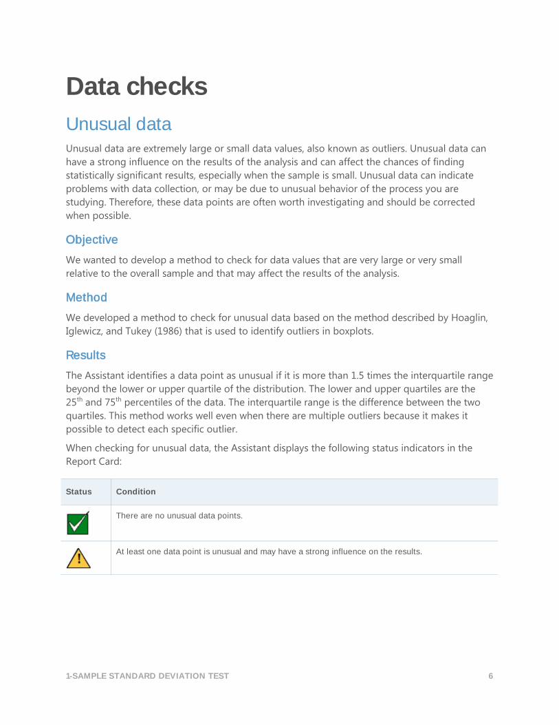
Unusual data Unusual data are extremely large or small data values, also known as outliers. Unusual data can
have a strong influence on the results of the analysis and can affect the chances of finding
statistically significant results, especially when the sample is small. Unusual data can indicate
problems with data collection, or may be due to unusual behavior of the process you are
studying. Therefore, these data points are often worth investigating and should be corrected
when possible.
Objective
We wanted to develop a method to check for data values that are very large or very small
relative to the overall sample and that may affect the results of the analysis.
Method
We developed a method to check for unusual data based on the method described by Hoaglin,
Iglewicz, and Tukey (1986) that is used to identify outliers in boxplots.
Results
The Assistant identifies a data point as unusual if it is more than 1.5 times the interquartile range
beyond the lower or upper quartile of the distribution. The lower and upper quartiles are the
25th and 75th percentiles of the data. The interquartile range is the difference between the two
quartiles. This method works well even when there are multiple outliers because it makes it
possible to detect each specific outlier.
When checking for unusual data, the Assistant displays the following status indicators in the
Report Card:
Status Condition
There are no unusual data points.
At least one data point is unusual and may have a strong influence on the results.
1-SAMPLE STANDARD DEVIATION TEST 7
Validity of test In the 1-Sample Standard Deviation Methods section above, we showed that Bonett’s method
generally provides better results than the AdjDF method. However, when the tails of a
distribution are heavier, Bonett’s method requires larger sample sizes to achieve accurate
results. Thus, a method for assessing the validity of the test must be based on not only the
sample size but also on the heaviness of the tails of the parent distribution. Gel et al. (2007)
developed a test to determine whether a sample comes from a distribution with heavy tails. This
test, called the SJ test, is based on the ratio of the sample standard deviation (s) and the tail
estimator J (for details, see Appendix E).
Objective
For a given sample of data, we needed to develop a rule to assess the validity of Bonett’s
method by evaluating the heaviness of the tails in the data.
Method
We performed simulations to investigate the power of the SJ test to identify heavy-tailed
distributions. If the SJ test is powerful for moderately large samples, then it can be used to
discriminate between heavy-tailed and light-tailed distributions for our purposes. For more
details, see Appendix F.
Results
Our simulations showed that when samples are large enough, the SJ test can be used to
discriminate between heavy-tailed and light-tailed distributions. For samples of moderate or
large size, smaller p-values indicate heavier tails and larger p-values indicate lighter tails.
However, because larger samples tend to have smaller p-values than smaller samples, we also
consider the sample size when determining the heaviness of the tails. Therefore, we developed
our set of rules for the Assistant to classify the tails of the distribution for each sample based on
the both sample size and the p-value of the SJ test. To see the specific ranges of p-values and
sample sizes associated with light, moderate, and heavy-tailed distributions, see Appendix F.
Based on these results, the Assistant Report Card displays the following status indicators to
evaluate the validity of the 1-Standard Deviation test (Bonett’s method) for your sample data:
Status Condition
There is no evidence that your sample has heavy tails. Your sample size is large enough to reliably check for this condition.
OR
Your sample has moderately heavy or heavy tails. However, your sample size is large enough to compensate, so the p-value should be accurate.

1-SAMPLE STANDARD DEVIATION TEST 8
Status Condition
Your sample has moderately heavy or heavy tails. Your sample size is not large enough to compensate. Use caution when interpreting the results.
OR
Your sample is not large enough to reliably check for heavy tails. Use caution when interpreting the results.
Sample size Typically, a statistical hypothesis test is performed to gather evidence to reject the null
hypothesis of “no difference”. If the sample is too small, the power of the test may not be
adequate to detect a difference that actually exists, which results in a Type II error. It is therefore
crucial to ensure that the sample sizes are sufficiently large to detect practically important
differences with high probability.
Objective
If the data does not provide sufficient evidence to reject the null hypothesis, we want to
determine whether the sample sizes are large enough for the test to detect practical differences
of interest with high probability. Although the objective of sample size planning is to ensure that
sample sizes are large enough to detect important differences with high probability, they should
not be so large that meaningless differences become statistically significant with high
probability.
Method
The power and sample size analysis for the 1-Sample Standard Deviation test is based on the
theoretical power function of the test. This power function provides good estimates when data
have nearly normal tails or light tails, but may produce conservative estimates when the data
have heavy tails (see the simulation results summarized in Performance of Theoretical Power
Function in the 1-Sample Standard Deviation Methods section above).
Results
When the data does not provide enough evidence against the null hypothesis, the Assistant uses
the power function of the normal approximation test to calculate the practical differences that
can be detected with an 80% and a 90% probability for the given sample size. In addition, if the
user provides a particular practical difference of interest, the Assistant uses the power function
of the normal approximation test to calculate sample sizes that yield an 80% and a 90% chance
of detection of the difference.

1-SAMPLE STANDARD DEVIATION TEST 9
To help interpret the results, the Assistant Report Card for the 1-Sample Standard Deviation test
displays the following status indicators when checking for power and sample size:
Status Condition
The test finds a difference between the standard deviation and the target value, so power is not an issue.
OR
Power is sufficient. The test did not find a difference between the standard deviation and the target value, but the sample is large enough to provide at least a 90% chance of detecting the given difference.
Power may be sufficient. The test did not find a difference between the standard deviation and the target value, but the sample is large enough to provide an 80% to 90% chance of detecting the given difference. The sample size required to achieve 90% power is reported.
Power might not be sufficient. The test did not find a difference between the standard deviation and the target value, and the sample is large enough to provide a 60% to 80% chance of detecting the given difference. The sample sizes required to achieve 80% power and 90% power are reported.
Power is not sufficient. The test did not find a difference between the standard deviation and the target value, and the sample is not large enough to provide at least a 60% chance of detecting the given difference. The sample sizes required to achieve 80% power and 90% power are reported.
The test did not find a difference between the standard deviation and the target value. You did not specify a practical difference to detect. Depending on your data, the report may indicate the differences that you could detect with 80% and 90% chance, based on your sample size and alpha.

1-SAMPLE STANDARD DEVIATION TEST 10
References Bonett, D.G. (2006). Approximate confidence interval for standard deviation of nonnormal
distributions. Computational Statistics & Data Analysis, 50, 775-782.
Box, G.E.P. (1953). Non-normality and tests on variances. Biometrika,40, 318.
Efron, B., & Tibshirani, R. J. (1993). An introduction to the bootstrap. Boca Raton, FL: Chapman
and Hall/CRC.
Gel, Y. R., Miao, W., & Gastwirth, J. L. (2007). Robust directed tests of normality against heavy-
tailed alternatives. Computational Statistics & Data Analysis, 51, 2734-2746.
Hummel, R., Banga, S., & Hettmansperger, T.P. (2005). Better confidence intervals for the
variance in a random sample. Minitab Technical Report.
Lee, S.J., & Ping, S. (1996). Testing the variance of symmetric heavy-tailed distributions. Journal
of Statistical Computation and Simulation, 56, 39-52.

1-SAMPLE STANDARD DEVIATION TEST 11
Appendix A: Methods for testing variance (or standard deviation) The table below summarizes strengths and weaknesses associated with various methods for
testing the variance.
Method Comment
Classical chi-square procedure Extremely sensitive to normality assumption. Even small departures from normality can produce inaccurate results regardless of how large the sample is. In fact, when the data deviate from normality, increasing the sample size decreases the accuracy of the procedure.
Large-sample method based on the asymptotic normal distribution of the logarithmic-transform of the sample variance
Generally better than the classical chi-square method but requires larger sample sizes to be insensitive to the normality assumption.
Large-sample method based on Edgeworth expansion for one-sided (upper tail) tests
See Lee and Ping (1996).
Produces acceptable Type I error rates, but requires that data come from a symmetric distribution.
Large-sample method based on an approximation of the distribution of the sample variance by a scaled chi-square distribution. The method is referred to as the Adjusted degrees of freedom (AdjDF) method.
See Hummel, Banga, and Hettmansperger (2005).
Provides better coverage probability than the method based on the asymptotic normal distribution of the logarithmic-transform of the sample variance and the nonparametric ABC bootstrap approximation method for confidence intervals (Efron and Tibshirani, 1993).
Used for the 1 Variance test in Minitab 15.
distribution of the logarithmic-transform of the sample variance
See Bonett (2006).
Provides good coverage probability for confidence intervals even for moderately large samples. However, requires much larger samples when data come from heavy-tailed distributions.
Used for the 1 Variance test and the Assistant 1-Sample Standard Deviation test in Minitab 16.

1-SAMPLE STANDARD DEVIATION TEST 12
method and the AdjDF method Let 𝑥1, … , 𝑥𝑛 be an observed random sample of size 𝑛 from a population with a finite fourth
moment. Let �̅� and 𝑠 be the observed sample mean and standard deviation, respectively. Also,
let 𝛾 and 𝛾𝑒 be the population kurtosis and kurtosis excess, respectively, so that 𝛾𝑒 = 𝛾 − 3. Thus,
for a normal population, 𝛾 = 3 and 𝛾𝑒 = 0. Also, let 𝜎2 be the unknown population variance. In
the sections that follow, we present two methods for making an inference about 𝜎2, the
adjusted degrees of freedom (AdjDF) method and Bonett’s method.
Formula B1: AdjDF method The AdjDF method is based upon an approximation of the distribution of the sample variance by
a scaled chi-square distribution (see Box, 1953). More specifically, the first two moments of the
sample variance are matched with the moments of a scaled chi-square distribution to determine
the unknown scale and degrees of freedom. This approach yields the following approximate
two-sided (1 − 𝛼)100 percent confidence interval for the variance:
[𝑟𝑠2
𝜒𝑟,𝛼/22 ,
𝑟𝑠2
𝜒𝑟,1−𝛼/22 ]
where
𝑟 =2𝑛
𝛾𝑒 + 2𝑛/(𝑛 − 1)
𝛾𝑒 =𝑛(𝑛 + 1)
(𝑛 − 1)(𝑛 − 2)(𝑛 − 3)∑(
𝑥𝑖 − �̅�
𝑠)4𝑛
𝑖=1
−3(𝑛 − 1)2
(𝑛 − 2)(𝑛 − 3)
This estimate of the kurtosis excess is identical to the one used for the Basic Statistics
commands in Minitab.
method Bonett’s method relies on the well-known classical approach, which uses the central limit
theorem and the Cramer 𝛿 method to obtain an asymptotic distribution of the log-transform of
the sample variance. The log-transformation is used to accelerate convergence to normality.
Using this approach, the approximate two-sided (1 − 𝛼)100 percent confidence interval for the
variance is defined as:
[𝑠2 exp(−zα/2se) , 𝑠2 exp(zα/2se)]

1-SAMPLE STANDARD DEVIATION TEST 13
where 𝑧𝛼 is the upper percentile of the standard normal distribution, and 𝑠𝑒 is an asymptotic
estimate of the standard error of the log-transformed sample variance, given as:
𝑠𝑒 = √�̂�−(𝑛−3)/𝑛
𝑛−1= √
�̂�𝑒+2+3/𝑛
𝑛−1
Previously, Hummel et al. (2005) performed simulation studies that demonstrated that the AdjDF
method is superior to this classical approach. However, Bonett makes two adjustments to the
classical approach to overcome its limitations.
The first adjustment involves the estimate of the kurtosis. To estimate kurtosis, Bonett uses the
following formula:
𝛾𝑒 =𝑛
(𝑛 − 1)2∑(
𝑥𝑖 −𝑚
𝑠)4
𝑛
𝑖=1
− 3
where 𝑚 is a trimmed mean with trim-proportion equal to 1/2√𝑛 − 4. This estimate of kurtosis
tends to improve the accuracy of the confidence levels for heavy-tailed (symmetric or skewed)
distributions.
For the second adjustment, Bonett empirically determines a constant multiplier for the sample
variance and the standard error. This constant multiplier approximately equalizes the tail
probabilities when the sample is small, and is given as:
𝑐 =𝑛
𝑛 − 𝑧𝛼/2
These adjustments yield Bonett’s approximate two-sided (1 − 𝛼)100 percent confidence interval
for the variance:
[𝑐𝑠2exp (−c zα/2se), 𝑐𝑠2exp (c zα/2se)]

1-SAMPLE STANDARD DEVIATION TEST 14
method versus AdjDF method
Simulation C1: Comparison of confidence intervals We wanted to compare the accuracy of the confidence intervals for the variance that are
calculated using AdjDF method and Bonett’s method. We generated random samples of
different sizes (𝑛 = 20, 30, 40, 50, 60, 80, 100, 150, 200, 250, 300) from several distributions and
calculated the confidence intervals using each method. The distributions included:
Standard normal distribution (N(0,1))
Symmetric and light-tailed distributions, including the uniform distribution (U(0,1)) and
the Beta distribution with both parameters set to 3 (B(3,3))
Symmetric and heavy-tailed distributions, including t-distributions with 5 and 10 degrees
of freedom (t(5),t(10)), and the Laplace distribution with location 0 and scale 1 (Lpl))
Skewed and heavy-tailed distributions, including the exponential distribution with scale 1
(Exp) and chi-square distributions with 3, 5, and 10 degrees of freedom (Chi(3), Chi(5),
Chi(10))
Left-skewed and heavy-tailed distribution; specifically, the Beta distribution with the
parameters set to 8 and 1, respectively (B(8,1))
In addition, to assess the direct effect of outliers, we generated samples from contaminated
normal distributions defined as
𝐶𝑁(𝑝, 𝜎) = 𝑝𝑁(0,1) + (1 − 𝑝)𝑁(0, 𝜎)
where 𝑝 is the mixing parameter and 1 − 𝑝 is the proportion of contamination (which equals the
proportion of outliers). We selected two contaminated normal populations for the study:
𝐶𝑁(0.9,3), where 10% of the population are outliers; and 𝐶𝑁(0.8,3), where 20% of the
population are outliers. These two distributions are symmetric and have long tails due to the
outliers.
For each sample size, 10,000 sample replicates were drawn from each distribution and the two-
sided 95% confidence intervals were calculated using each method. The random sample
generator was seeded so that both methods were applied to the same samples. Based on these
confidence intervals, we then calculated the simulated coverage probabilities (CovP) and
average interval widths (AveW) for each method. If the confidence intervals of the two methods
have about the same simulated coverage probabilities, then the method that produces shorter
intervals (on average) is more precise. Because we used a target confidence level of 95%, the
simulation error was √0.95(0.05)/10,000 = 0.2%.
The simulation results are recorded in Tables 1 and 2 below.

1-SAMPLE STANDARD DEVIATION TEST 15
Table 1 Simulated coverage probabilities of 95% two-sided confidence intervals for the variance
calculated using the AdjDF and Bonett’s methods. These samples were generated from
symmetric distributions with light, normal, nearly normal, or heavy tails.
Distribution
Symmetric Distributions with Light, Normal, or Nearly Normal Tails
Symmetric Distributions with Heavy Tails
U(0,1) B(3,3) N(0,1) t(10) Lpl CN(0.8, 3)
CN (0.9, 3)
T(5)
Skewness 0 0 0 0 0 0 0 0
Kurtosis (𝜸𝒆) -1.200 -0.667 0 1.000 3.000 4.544 5.333 6.000
𝒏 = 𝟏𝟎
AdjDF CovP
AveW
0.910
0.154
0.909
0.087
0.903
3.276
0.883
5.160
0.853
13.924
0.793
21.658
0.815
14.913
0.858
11.742
Bonett CovP
AveW
0.972
0.242
0.967
0.115
0.962
3.710
0.952
5.134
0.919
10.566
0.891
15.335
0.920
10.367
0.935
8.578
𝒏 = 𝟐𝟎
AdjDF CovP
AveW
0.937
0.080
0.937
0.045
0.923
1.572
0.909
2.463
0.881
5.781
0.819
9.265
0.817
6.539
0.868
5.151
Bonett CovP
AveW
0.953
0.100
0.954
0.051
0.946
1.683
0.934
2.422
0.909
4.932
0.856
7.282
0.864
4.945
0.904
4.026
𝒏 = 𝟑𝟎
AdjDF CovP
AveW
0.946
0.061
0.942
0.034
0.933
1.170
0.917
1.764
0.894
4.117
0.851
6.330
0.823
4.557
0.882
3.667
Bonett CovP
AveW
0.951
0.070
0.950
0.037
0.947
1.221
0.933
1.750
0.909
3.654
0.869
5.383
0.852
3.736
0.907
2.997
𝒏 = 𝟒𝟎
AdjDF CovP
AveW
0.953
0.051
0.947
0.028
0.932
0.971
0.922
1.489
0.904
3.246
0.867
5.131
0.833
3.654
0.890
3.024
Bonett CovP
AveW
0.954
0.057
0.951
0.030
0.941
1.002
0.936
1.469
0.914
2.994
0.879
4.519
0.856
3.128
0.907
2.542

1-SAMPLE STANDARD DEVIATION TEST 16
Distribution
Symmetric Distributions with Light, Normal, or Nearly Normal Tails
Symmetric Distributions with Heavy Tails
U(0,1) B(3,3) N(0,1) t(10) Lpl CN(0.8, 3)
CN (0.9, 3)
T(5)
Skewness 0 0 0 0 0 0 0 0
Kurtosis (𝜸𝒆) -1.200 -0.667 0 1.000 3.000 4.544 5.333 6.000
𝒏 = 𝟓𝟎
AdjDF CovP
AveW
0.951
0.045
0.945
0.025
0.937
0.849
0.925
1.291
0.911
2.789
0.878
4.357
0.838
3.091
0.893
2.603
Bonett CovP
AveW
0.951
0.049
0.947
0.026
0.944
0.870
0.938
1.280
0.918
2.613
0.888
3.939
0.855
2.729
0.908
2.240
𝒏 = 𝟔𝟎
AdjDF CovP
AveW
0.949
0.040
0.943
0.022
0.938
0.766
0.926
1.155
0.913
2.490
0.890
3.857
0.853
2.768
0.899
2.283
Bonett CovP
AveW
0.949
0.043
0.947
0.023
0.943
0.781
0.935
1.147
0.918
2.354
0.896
3.552
0.868
2.498
0.910
2.023
𝒏 = 𝟕𝟎
AdjDF CovP
AveW
0.948
0.037
0.945
0.020
0.940
0.701
0.930
1.056
0.913
2.283
0.890
3.458
0.858
2.475
0.896
2.049
Bonett CovP
AveW
0.947
0.039
0.946
0.021
0.944
0.713
0.938
1.049
0.918
2.174
0.894
3.227
0.868
2.272
0.905
1.828
𝒏 = 𝟖𝟎
AdjDF CovP
AveW
0.947
0.034
0.949
0.019
0.938
0.652
0.929
0.988
0.918
2.089
0.905
3.205
0.869
2.300
0.902
1.906
Bonett CovP
AveW
0.946
0.036
0.950
0.019
0.942
0.662
0.935
0.982
0.923
2.005
0.907
3.014
0.877
2.133
0.911
1.716
𝒏 = 𝟗𝟎
AdjDF CovP
AveW
0.946
0.032
0.947
0.018
0.948
0.611
0.929
0.921
0.918
1.951
0.908
2.982
0.869
2.124
0.901
1.874
Bonett CovP
AveW
0.945
0.034
0.948
0.018
0.952
0.618
0.936
0.916
0.920
1.882
0.910
2.822
0.874
1.984
0.909
1.646

1-SAMPLE STANDARD DEVIATION TEST 17
Distribution
Symmetric Distributions with Light, Normal, or Nearly Normal Tails
Symmetric Distributions with Heavy Tails
U(0,1) B(3,3) N(0,1) t(10) Lpl CN(0.8, 3)
CN (0.9, 3)
T(5)
Skewness 0 0 0 0 0 0 0 0
Kurtosis (𝜸𝒆) -1.200 -0.667 0 1.000 3.000 4.544 5.333 6.000
𝒏 = 𝟏𝟎𝟎
AdjDF CovP
AveW
0.947
0.030
0.951
0.017
0.945
0.576
0.933
0.873
0.920
1.830
0.910
2.801
0.885
2.017
0.912
1.658
Bonett CovP
AveW
0.946
0.032
0.953
0.017
0.948
0.583
0.937
0.869
0.923
1.772
0.912
2.666
0.891
1.899
0.916
1.522
𝒏 = 𝟏𝟓𝟎
AdjDF CovP
AveW
0.949
0.024
0.951
0.014
0.947
0.464
0.936
0.700
0.932
1.470
0.925
2.228
0.896
1.602
0.912
1.325
Bonett CovP
AveW
0.948
0.025
0.952
0.014
0.949
0.467
0.939
0.698
0.933
1.438
0.924
2.156
0.898
1.539
0.915
1.251
𝒏 = 𝟐𝟎𝟎
AdjDF CovP
AveW
0.943
0.021
0.949
0.012
0.948
0.400
0.938
0.605
0.927
1.265
0.930
1.906
0.914
1.373
0.918
1.178
Bonett CovP
AveW
0.942
0.021
0.951
0.012
0.949
0.402
0.940
0.603
0.928
1.245
0.930
1.860
0.915
1.333
0.920
1.106
𝒏 = 𝟐𝟓𝟎
AdjDF CovP
AveW
0.952
0.019
0.952
0.010
0.949
0.355
0.942
0.538
0.938
1.120
0.929
1.690
0.909
1.219
0.915
1.037
Bonett CovP
AveW
0.951
0.019
0.952
0.010
0.949
0.357
0.944
0.537
0.941
1.106
0.929
1.657
0.909
1.190
0.916
0.986
𝒏 = 𝟑𝟎𝟎
AdjDF CovP
AveW
0.950
0.017
0.948
0.009
0.951
0.324
0.940
0.490
0.938
1.019
0.936
1.544
0.920
1.115
0.914
0.933
Bonett CovP
AveW
0.950
0.017
0.947
0.010
0.951
0.325
0.942
0.489
0.937
1.009
0.929
1.657
0.920
1.093
0.916
0.897

1-SAMPLE STANDARD DEVIATION TEST 18
Table 2 Simulated coverage probabilities of 95% two-sided confidence intervals for the variance
calculated using the AdjDF and Bonett’s methods. These samples were generated from skew
distributions with nearly normal, moderately heavy, or heavy tails.
Distribution Skew Distributions with Nearly Normal or Moderately Heavy Tails
Skew Distributions with Heavy Tails
Chi(10) B(8,1) Chi(5) Chi(3) Exp
Skewness 0.894 -1.423 1.265 1.633 2
Kurtosis (𝜸𝒆) 1.200 2.284 2.400 4.000 6
𝒏 = 𝟏𝟎
AdjDF CovP
AveW
0.869
93.383
0.815
0.065
0.836
61.994
0.797
47.821
0.758
10.711
Bonett CovP
AveW
0.950
91.006
0.917
0.058
0.938
53.830
0.911
38.137
0.882
7.498
𝒏 = 𝟐𝟎
AdjDF CovP
AveW
0.889
41.497
0.862
0.026
0.862
25.479
0.833
20.099
0.811
4.293
Bonett CovP
AveW
0.932
41.600
0.912
0.026
0.913
24.094
0.893
17.232
0.877
3.370
𝒏 = 𝟑𝟎
AdjDF CovP
AveW
0.901
30.021
0.881
0.018
0.880
18.182
0.864
13.630
0.838
2.844
Bonett CovP
AveW
0.931
30.462
0.920
0.019
0.914
17.858
0.906
12.634
0.885
2.441
𝒏 = 𝟒𝟎
AdjDF CovP
AveW
0.909
24.459
0.882
0.015
0.885
14.577
0.867
10.649
0.862
2.193
Bonett CovP
AveW
0.930
24.952
0.915
0.015
0.913
14.504
0.904
1.991
0.898
1.991

1-SAMPLE STANDARD DEVIATION TEST 19
Distribution Skew Distributions with Nearly Normal or Moderately Heavy Tails
Skew Distributions with Heavy Tails
Chi(10) B(8,1) Chi(5) Chi(3) Exp
Skewness 0.894 -1.423 1.265 1.633 2
Kurtosis (𝜸𝒆) 1.200 2.284 2.400 4.000 6
𝒏 = 𝟓𝟎
AdjDF CovP
AveW
0.912
21.373
0.900
0.013
0.892
12.694
0.871
9.115
0.868
1.861
Bonett CovP
AveW
0.930
21.814
0.927
0.013
0.916
12.741
0.903
8.897
0.901
1.735
𝒏 = 𝟔𝟎
AdjDF CovP
AveW
0.915
18.928
0.908
0.011
0.901
11.338
0.890
8.211
0.875
1.645
Bonett CovP
AveW
0.930
19.369
0.933
0.012
0.923
11.456
0.917
8.093
0.900
1.554
𝒏 = 𝟕𝟎
AdjDF CovP
AveW
0.915
17.513
0.910
0.010
0.904
10.307
0.898
7.461
0.881
1.488
Bonett CovP
AveW
0.932
17.906
0.932
0.011
0.922
10.464
0.919
7.408
0.906
1.429
𝒏 = 𝟖𝟎
AdjDF CovP
AveW
0.920
16.157
0.916
0.009
0.911
9.604
0.904
6.892
0.890
1.349
Bonett CovP
AveW
0.935
16.537
0.936
0.010
0.929
9.765
0.924
6.882
0.915
1.314
𝒏 = 𝟗𝟎
AdjDF CovP
AveW
0.924
15.250
0.918
0.009
0.911
9.007
0.897
6.323
0.894
1.255
Bonett CovP
AveW
0.938
15.609
0.936
0.009
0.929
9.175
0.918
6.366
0.913
1.230

1-SAMPLE STANDARD DEVIATION TEST 20
Distribution Skew Distributions with Nearly Normal or Moderately Heavy Tails
Skew Distributions with Heavy Tails
Chi(10) B(8,1) Chi(5) Chi(3) Exp
Skewness 0.894 -1.423 1.265 1.633 2
Kurtosis (𝜸𝒆) 1.200 2.284 2.400 4.000 6
𝒏 = 𝟏𝟎𝟎
AdjDF CovP
AveW
0.926
14.332
0.919
0.008
0.915
8.451
0.908
6.016
0.895
1.171
Bonett CovP
AveW
0.935
14.664
0.936
0.009
0.931
8.625
0.924
6.063
0.916
1.158
𝒏 = 𝟏𝟓𝟎
AdjDF CovP
AveW
0.933
11.606
0.925
0.007
0.923
6.781
0.913
4.792
0.911
0.933
Bonett CovP
AveW
0.943
11.846
0.941
0.007
0.936
6.942
0.929
4.875
0.928
0.937
𝒏 = 𝟐𝟎𝟎
AdjDF CovP
AveW
0.935
9.973
0.934
0.006
0.926
5.849
0.916
4.127
0.915
0.799
Bonett CovP
AveW
0.942
10.185
0.948
0.006
0.936
5.991
0.930
4.212
0.931
0.808
𝒏 = 𝟐𝟓𝟎
AdjDF CovP
AveW
0.938
8.899
0.939
0.005
0.934
5.231
0.926
3.652
0.922
0.705
Bonett CovP
AveW
0.946
9.078
0.951
0.005
0.944
5.355
0.936
3.735
0.931
0.716
𝒏 = 𝟑𝟎𝟎
AdjDF CovP
AveW
0.942
8.156
0.938
0.005
0.934
4.749
0.931
3.344
0.922
0.640
Bonett CovP
AveW
0.947
8.314
0.948
0.005
0.943
4.862
0.941
3.419
0.933
0.651

1-SAMPLE STANDARD DEVIATION TEST 21
Our results are very consistent with those published by Bonett (2006). As shown in Tables 1 and
2, the confidence intervals calculated using Bonett’s method are superior to the confidence
intervals calculated using the AdjDF method because they yield coverage probabilities closer to
the target level of 0.95 and narrower confidence intervals, on average. If the confidence intervals
of the two methods have about the same simulated coverage probabilities, then the method
that produces shorter intervals (on average) is more precise. This means that the statistical test
for the variance based on Bonett’s method performs better and results in lower Type I and Type
II error rates. When sample sizes are large, the two methods yield almost identical results, but
for small to moderate sample sizes, Bonett’s method is superior.
Although Bonett’s method generally performs better than the AdjDF method, it consistently
yields coverage probabilities below the target coverage of 0.95 for heavy-tailed distributions
(symmetric or skewed) even for extremely large samples (𝑛 > 100). This is illustrated in Figure 1
below, which plots the simulated coverage probabilities for Bonett’s method against the true
kurtosis excess of the population for small, moderate, and large sample sizes.
Figure 1 Simulated coverage probabilities for Bonett’s 95% confidence intervals plotted against
the kurtosis excess of each distribution at various sample sizes.
As shown in Figure 1, the greater the kurtosis, the larger the sample size that is needed to make
the simulated coverage probabilities approach the target level. As noted previously, the
simulated coverage probabilities for Bonett’s method are low for heavy-tailed distributions.
However, for lighter tailed distributions, such as the uniform and the Beta(3,3) distributions, the
5.02.50.0
0.950
0.925
0.900
0.875
0.850
5.02.50.0
0.950
0.925
0.900
0.875
0.850
5.02.50.0
20
Kurtosis Excess
Co
vera
ge p
rob
ab
ilit
y
0.95
50 100
150 200 250
0.95
Panel variable: N
Simulated Coverage Probability vs True Kurtosis Excess

1-SAMPLE STANDARD DEVIATION TEST 22
simulated coverage probabilities are stable and on target for sample sizes as small as 20.
Therefore, we base our criterion to determine the validity of Bonett’s method upon both the
sample size and the heaviness of the tails of the distribution from which the sample is drawn.
As a first step for developing this criterion, we classify the distributions into three categories
according to the heaviness of their tails:
Light-tailed or normal-tailed distributions (L-type): These are distributions for which
Bonett’s confidence intervals yield stable coverage probabilities near the target coverage
level. For these distributions, sample sizes as low as 20 produce accurate results.
Examples include the uniform distribution, the Beta(3,3) distribution, the normal
distribution, the t distribution with 10 degrees of freedom, and the chi-square
distribution with 10 degrees of freedom.
Moderately heavy-tailed distributions (M-type): For these distributions, Bonett’s
method requires a minimum sample size of 80 for the simulated coverage probabilities
to be close to the target coverage. Examples include the chi-square distribution with 5
degrees of freedom, and the Beta(8,1) distribution.
Heavy-tailed distributions (H-type): These are distributions for which Bonett’s
confidence intervals yield coverage probabilities that are far below the targeted
coverage, unless the sample sizes are extremely large (𝑛 ≥ 200). Examples include the t
distribution with 5 degrees of freedom, the Laplace distribution, the chi-square
distribution with 3 degrees of freedom, the exponential distribution, and the two
contaminated normal distributions, CN(0.9,3) and CN(0.8,3).
Thus, a general rule for evaluating the validity of Bonett’s method requires that we develop a
procedure to identify which of the 3 distribution types the sample data comes from. We
developed this procedure as part of the Validity of test data check. For more details, see
Appendix E.

1-SAMPLE STANDARD DEVIATION TEST 23
Appendix D: Theoretical power We derived the theoretical power function of the test associated with Bonett’s method and
performed simulations to compare the theoretical and simulated power of the test. If the
theoretical and simulated power curves are close to each other, then the power and sample size
analysis based upon on the theoretical power function should yield accurate results.
method As described earlier, Bonett’s method is based upon the well-known classical approach, in which
the central limit theorem and the Cramer 𝛿 method are used to find an asymptotic distribution
of the log-transformed sample variance. More specifically, it is established that in large samples,
ln 𝑆2−ln𝜎2
𝑠𝑒 is approximately distributed as the standard normal distribution. The denominator,
𝑠𝑒, is the large sample standard error of the log-transformed sample variance and is given as
𝑠𝑒 = √𝛾−(𝑛−3)/𝑛
𝑛−1
where 𝛾 is the kurtosis of the unknown parent population.
It follows that an approximate power function with an approximate alpha level for the two-sided
test using Bonett’s method may be given as a function of the sample size, the ratio 𝜌 = 𝜎/𝜎0
and the parent population kurtosis 𝛾 as
𝜋(𝑛, 𝜌, 𝛾) = 1 −Φ
(
𝑧𝛼/2 −ln 𝜌2
√𝛾 − 1 + 3/𝑛𝑛 − 1 )
+Φ
(
−𝑧𝛼/2 −ln𝜌2
√𝛾 − 1 + 3/𝑛𝑛 − 1 )
where 𝜎0 is the hypothesized value of the unknown standard deviation, Φ is the CDF of the
standard normal distribution, and 𝑧𝛼 is the upper α percentile point of the standard normal
distribution. The one-sided power functions can also be obtained from these calculations.
Note that when planning the sample size for a study, an estimate of the kurtosis may be used in
place of the true kurtosis. This estimate is usually based on the opinions of experts or the results
of previous experiments. If that information is not available, it is often a good practice to
perform a small pilot study to develop the plans for the major study. Using a sample from the
pilot study, the kurtosis may be estimated as
𝛾 =𝑛
(𝑛 − 1)2∑(
𝑥𝑖 −𝑚
𝑠)4
𝑛
𝑖=1
where 𝑚 is a trimmed mean with trim-proportion equal to 1/2√𝑛 − 4.

1-SAMPLE STANDARD DEVIATION TEST 24
Simulation D1: Comparison of actual power versus theoretical power We designed a simulation to compare estimated actual power levels (referred to as simulated
power levels) to the theoretical power levels (referred to as approximate power levels) when
using Bonett’s method to test the variance.
In each experiment, we generated 10,000 sample replicates, each of size 𝑛, where 𝑛 =
20, 30, 40, 50,… ,120, from each of the distributions described in Simulation C1 (see Appendix C).
For each distribution and sample size 𝑛, we calculated the simulated power level as the fraction
of 10,000 random sample replicates for which the two-sided test with alpha level 𝛼 = 0.05 was
significant. When calculating the simulated power, we used 𝜌 = 𝜎/𝜎0 = 1.25 to obtain relatively
small power levels. We then calculated the corresponding power levels using the theoretical
power function for comparison.
The results are shown in Tables 3 and 4 and graphically represented in Figure 2 below.
Table 3 Simulated power levels (evaluated at 𝜌 = 𝜎/𝜎0 = 1.25) of a two-sided test for the
variance based on Bonett’s method compared with theoretical (normal approximation) power
levels. The samples were generated from symmetric distributions with light, normal, nearly
normal, or heavy tails.
𝒏 Power Symmetric Distributions with Light, Normal, or Nearly Normal Tails
Symmetric Distributions with Heavy Tails
U(0,1) B(3,3) N(0,1) t(10) Lpl CN (.8,3)
CN (.9,3)
t(5)
20 Simul.
Approx.
0.521
0.514
0.390
0.359
0.310
0.264
0.237
0.195
0.178
0.137
0.152
0.117
0.139
0.109
0.172
0.104
30 Simul.
Approx.
0.707
0.717
0.551
0.519
0.441
0.382
0.337
0.276
0.225
0.186
0.186
0.154
0.169
0.143
0.228
0.135
40 Simul.
Approx.
0.831
0.846
0.679
0.651
0.526
0.490
0.427
0.356
0.285
0.236
0.266
0.192
0.203
0.176
0.285
0.165
50 Simul.
Approx.
0.899
0.921
0.753
0.754
0.621
0.586
0.505
0.431
0.332
0.284
0.255
0.229
0.238
0.210
0.340
0.196
60 Simul.
Approx.
0.942
0.961
0.822
0.830
0.701
0.668
0.570
0.501
0.380
0.332
0.285
0.266
0.274
0.243
0.384
0.227
70 Simul.
Approx.
0.964
0.981
0.866
0.885
0.757
0.737
0.632
0.566
0.424
0.379
0.327
0.303
0.314
0.276
0.439
0.257

1-SAMPLE STANDARD DEVIATION TEST 25
𝒏 Power Symmetric Distributions with Light, Normal, or Nearly Normal Tails
Symmetric Distributions with Heavy Tails
U(0,1) B(3,3) N(0,1) t(10) Lpl CN (.8,3)
CN (.9,3)
t(5)
80 Simul.
Approx.
0.981
0.991
0.909
0.923
0.815
0.794
0.689
0.624
0.481
0.423
0.372
0.340
0.347
0.309
0.483
0.288
90 Simul.
Approx.
0.988
0.996
0.937
0.950
0.851
0.840
0.724
0.676
0.514
0.467
0.400
0.375
0.377
0.342
0.523
0.318
100 Simul.
Approx.
0.994
0.998
0.961
0.967
0.880
0.876
0.779
0.722
0.558
0.508
0.430
0.410
0.411
0.373
0.566
0.347
110 Simul.
Approx.
0.997
0.999
0.967
0.979
0.909
0.905
0.803
0.763
0.591
0.547
0.471
0.443
0.449
0.404
0.592
0.376
120 Simul.
Approx.
0.999
1.000
0.982
0.987
0.929
0.928
0.844
0.799
0.629
0.584
0.502
0.476
0.476
0.434
0.630
0.405
Table 4 Simulated power levels (evaluated at 𝜌 = 𝜎/𝜎0 = 1.25 ) of a two-sided test for the
variance based on Bonett’s method compared with theoretical (normal approximation) power
levels. The samples were generated from skew distributions with nearly normal, moderately
heavy, or heavy tails.
𝒏 Power Skewed Distributions with Nearly Normal or Moderately Heavy Tails
Skewed Distributions with Heavy Tails
Chi(10) B(8,1) Chi(5) Chi(3) Exp
20 Simul.
Approx.
0.222
0.186
0.166
0.152
0.172
0.149
0.139
0.123
0.128
0.104
30 Simul.
Approx.
0.314
0.263
0.216
0.263
0.234
0.205
0.190
0.164
0.151
0.135
40 Simul.
Approx.
0.387
0.338
0.266
0.266
0.292
0.261
0.223
0.204
0.186
0.165
50 Simul.
Approx.
0.455
0.409
0.324
0.323
0.349
0.316
0.263
0.245
0.208
0.196
60 Simul.
Approx.
0.521
0.477
0.376
0.377
0.399
0.369
0.302
0.286
0.239
0.227

1-SAMPLE STANDARD DEVIATION TEST 26
𝒏 Power Skewed Distributions with Nearly Normal or Moderately Heavy Tails
Skewed Distributions with Heavy Tails
Chi(10) B(8,1) Chi(5) Chi(3) Exp
70 Simul.
Approx.
0.583
0.539
0.419
0.430
0.463
0.420
0.361
0.325
0.269
0.257
80 Simul.
Approx.
0.646
0.597
0.473
0.479
0.499
0.469
0.394
0.365
0.299
0.288
90 Simul.
Approx.
0.688
0.649
0.517
0.526
0.561
0.516
0.428
0.403
0.327
0.318
100 Simul.
Approx.
0.738
0.695
0.561
0.571
0.591
0.560
0.469
0.440
0.368
0.347
110 Simul.
Approx.
0.779
0.737
0.608
0.611
0.637
0.600
0.495
0.475
0.394
0.376
120 Simul.
Approx.
0.810
0.774
0.635
0.650
0.679
0.638
0.538
0.509
0.416
0.405

1-SAMPLE STANDARD DEVIATION TEST 27
Figure 2 Simulated power curves compared with theoretical power curves for various
distributions
The results in Tables 3 and 4 and Figure 2 show that when samples are generated from
distributions with lighter tails (L-type distributions, as defined in Appendix C), such as the
uniform distribution, the Beta (3,3) distribution, the normal distribution, the t distribution with 10
degrees of freedom, and the chi-square distribution with 10 degrees of freedom, the theoretical
power values and the simulated power levels are practically undistinguishable.
However, for distributions with heavy tails (H-type distributions), the simulated power curves are
markedly above the theoretical power curves when the samples are small. These heavy-tailed
distributions include the t distribution with 5 degrees of freedom, the Laplace distribution, the
chi-square distribution with 3 degrees of freedom, the exponential distribution, and the two
contaminated normal distributions, CN(0.9,3) and CN(0.8,3). Therefore, when planning the
sample size for a study and the sample comes from a distribution with heavy tails, the sample
size estimated by the theoretical power function may be larger than the actual sample size
required to achieve a given target power.

1-SAMPLE STANDARD DEVIATION TEST 28
Appendix E: The SJ test for normal versus heavy tails The results of the simulation study in Appendix C showed that when the tails of the distribution
are heavier, larger sample sizes are required for the simulated coverage probability of Bonett’s
confidence intervals to approach the target level. Skewness, however, did not appear to have a
significant effect on the simulated coverage probabilities.
Therefore, we needed to develop a criterion to assess the validity of Bonett’s method based
both on the size of the sample and the heaviness of the tails of the distribution from which the
sample is drawn. Fortunately, Gel et al. (2007) provide a reasonably powerful test for directly
testing the null hypothesis that the distribution has normal tails against the alternative
hypothesis that the distribution has heavy tails. The test, which we refer to as the SJ test, is
based upon the following statistic:
�̂� =𝑠
𝑗̂
where 𝑆 is the sample standard deviation, 𝑗̂ is the estimate of the sample mean absolute
deviation from the median, 𝑚, and is given as
𝑗̂ =√𝜋/2
𝑛∑|𝑋𝑖
𝑛
𝑖=1
−𝑚|
An approximate size-𝛼 test against the alternative hypothesis of heavy tails rejects the null
hypothesis of normal tails if
√𝑛(�̂� − 1)
𝜎𝑅≥ 𝑧𝛼
where 𝑧𝛼is the upper 𝛼-percentile of a standard normal distribution and 𝜎𝑅 = (𝜋 − 3)/2.
Gel et al. (2007) have shown that replacing the upper 𝛼-percentile of the standard normal
distribution with that of the t distribution with (√𝑛 + 3)/2 degrees of freedom provides better
approximations for moderate sample sizes. Therefore, when applying the SJ test for the Validity
of test data check, we replace 𝑧𝛼with 𝑡𝑑,𝛼, the upper 𝛼-percentile of the t-distribution with 𝑑 =
(√𝑛 + 3)/2 degrees of freedom.

1-SAMPLE STANDARD DEVIATION TEST 29
Appendix F: Validity of test
Simulation F1: Using simulated power of SJ test to determine distribution classifications We performed simulations to investigate the power of the SJ test. We generated samples of
various sizes (𝑛 = 10, 20, 30, 40, 50, 60, 70, 80, 90, 100, 120, 140, 160, 180, 200) from various
distributions. The distributions had normal, light, moderate, or heavy tails, and are the same as
those described in simulation C1 (see Appendix C). For each given sample size, 10,000 sample
replicates were drawn from each distribution. We calculated the simulated power of the SJ test
as the proportion of cases for which the null hypothesis (that the parent distribution has normal
tails) was rejected. In addition, we calculated the average 𝑅 values (AveR) and the average p-
values (AvePV).
The simulation results are shown in Tables 5 and 6 below.
Table 5 Simulated power levels of the SJ test. The samples were generated from symmetric
distributions with light, normal, nearly normal, or heavy tails.
Distribution Symmetric Distributions with Light, Normal, or Nearly Normal Tails
Symmetric Distributions with Heavy Tails
U(0,1) B(3,3) N(0,1) t(10) Lpl CN (.8,3)
CN (.9,3)
t(5)
𝒏 TrueR 0.921 0.965 1.0 1.032 1.128 1.152 1.118 1.085
10 Power
AveR
AvePV
0.021
1.010
0.482
0.041
1.036
0.401
0.075
1.060
0.341
0.103
1.073
0.314
0.249
1.129
0.219
0.264
1.131
0.228
0.198
1.106
0.272
0.161
1.096
0.278
15 Power
AveR
AvePV
0.009
0.986
0.572
0.027
1.018
0.440
0.071
1.043
0.357
0.121
1.063
0.302
0.350
1.130
0.171
0.389
1.140
0.181
0.283
1.110
0.240
0.215
1.093
0.247
20 Power
AveR
AvePV
0.002
0.966
0.669
0.016
1.001
0.503
0.066
1.030
0.382
0.144
1.054
0.311
0.428
1.127
0.147
0.465
1.137
0.161
0.331
1.104
0.236
0.253
1.086
0.244
25 Power
AveR
AvePV
0.002
0.959
0.721
0.011
0.995
0.535
0.065
1.025
0.391
0.153
1.050
0.305
0.500
1.128
0.120
0.550
1.141
0.128
0.397
1.107
0.208
0.293
1.086
0.223

1-SAMPLE STANDARD DEVIATION TEST 30
Distribution Symmetric Distributions with Light, Normal, or Nearly Normal Tails
Symmetric Distributions with Heavy Tails
U(0,1) B(3,3) N(0,1) t(10) Lpl CN (.8,3)
CN (.9,3)
t(5)
𝒏 TrueR 0.921 0.965 1.0 1.032 1.128 1.152 1.118 1.085
30 Power
AveR
AvePV
0.001
0.951
0.773
0.010
0.989
0.570
0.060
1.019
0.409
0.170
1.046
0.304
0.561
1.127
0.103
0.603
1.141
0.112
0.431
1.106
0.197
0.334
1.084
0.209
40 Power
AveR
AvePV
0.000
0.944
0.840
0.006
0.984
0.616
0.058
1.015
0.420
0.190
1.043
0.287
0.665
1.126
0.073
0.709
1.145
0.076
0.513
1.109
0.162
0.401
1.084
0.179
50 Power
AveR
AvePV
0.000
0.939
0.886
0.004
0.980
0.654
0.058
1.012
0.427
0.208
1.040
0.279
0.746
1.126
0.053
0.785
1.146
0.055
0.590
1.111
0.131
0.462
1.084
0.156
60 Power
AveR
AvePV
0.000
0.936
0.913
0.002
0.978
0.686
0.060
1.010
0.430
0.231
1.039
0.267
0.813
1.127
0.039
0.836
1.146
0.039
0.647
1.112
0.109
0.518
1.084
0.134
70 Power
AveR
AvePV
0.000
0.934
0.935
0.002
0.975
0.716
0.054
1.009
0.437
0.247
1.037
0.259
0.863
1.127
0.028
0.879
1.147
0.029
0.702
1.112
0.091
0.554
1.083
0.123
80 Power
AveR
AvePV
0.000
0.933
0.950
0.001
0.974
0.740
0.054
1.007
0.440
0.265
1.037
0.241
0.896
1.128
0.021
0.912
1.147
0.021
0.729
1.111
0.079
0.591
1.083
0.105
90 Power
AveR
AvePV
0.000
0.932
0.962
0.001
0.973
0.759
0.054
1.007
0.445
0.281
1.036
0.237
0.933
1.128
0.014
0.934
1.148
0.016
0.771
1.113
0.067
0.633
1.083
0.093
100 Power
AveR
AvePV
0.000
0.930
0.971
0.001
0.972
0.779
0.057
1.006
0.446
0.301
1.036
0.224
0.947
1.127
0.012
0.954
1.148
0.011
0.805
1.113
0.055
0.661
1.083
0.083
120 Power
AveR
AvePV
0.000
0.929
0.982
0.000
0.971
0.809
0.052
1.005
0.452
0.334
1.035
0.206
0.974
1.128
0.006
0.974
1.149
0.007
0.852
1.114
0.041
0.732
1.083
0.064

1-SAMPLE STANDARD DEVIATION TEST 31
Distribution Symmetric Distributions with Light, Normal, or Nearly Normal Tails
Symmetric Distributions with Heavy Tails
U(0,1) B(3,3) N(0,1) t(10) Lpl CN (.8,3)
CN (.9,3)
t(5)
𝒏 TrueR 0.921 0.965 1.0 1.032 1.128 1.152 1.118 1.085
140 Power
AveR
AvePV
0.000
0.928
0.989
0.000
0.971
0.834
0.052
1.004
0.454
0.336
1.034
0.192
0.986
1.127
0.004
0.988
1.150
0.003
0.894
1.116
0.027
0.785
1.084
0.048
160 Power
AveR
AvePV
0.000
0.927
0.993
0.000
0.970
0.858
0.054
1.004
0.457
0.402
1.034
0.177
0.993
1.128
0.002
0.992
1.150
0.002
0.916
1.114
0.021
0.819
1.084
0.040
180 Power
AveR
AvePV
0.000
0.926
0.995
0.000
0.969
0.874
0.052
1.003
0.461
0.416
1.034
0.167
0.998
1.128
0.001
0.996
1.149
0.001
0.934
1.115
0.016
0.853
1.084
0.033
200 Power
AveR
AvePV
0.000
0.926
0.997
0.000
0.969
0.890
0.053
1.003
0.461
0.448
1.034
0.153
0.998
1.127
0.001
0.998
1.150
0.001
0.954
1.116
0.011
0.884
1.083
0.025
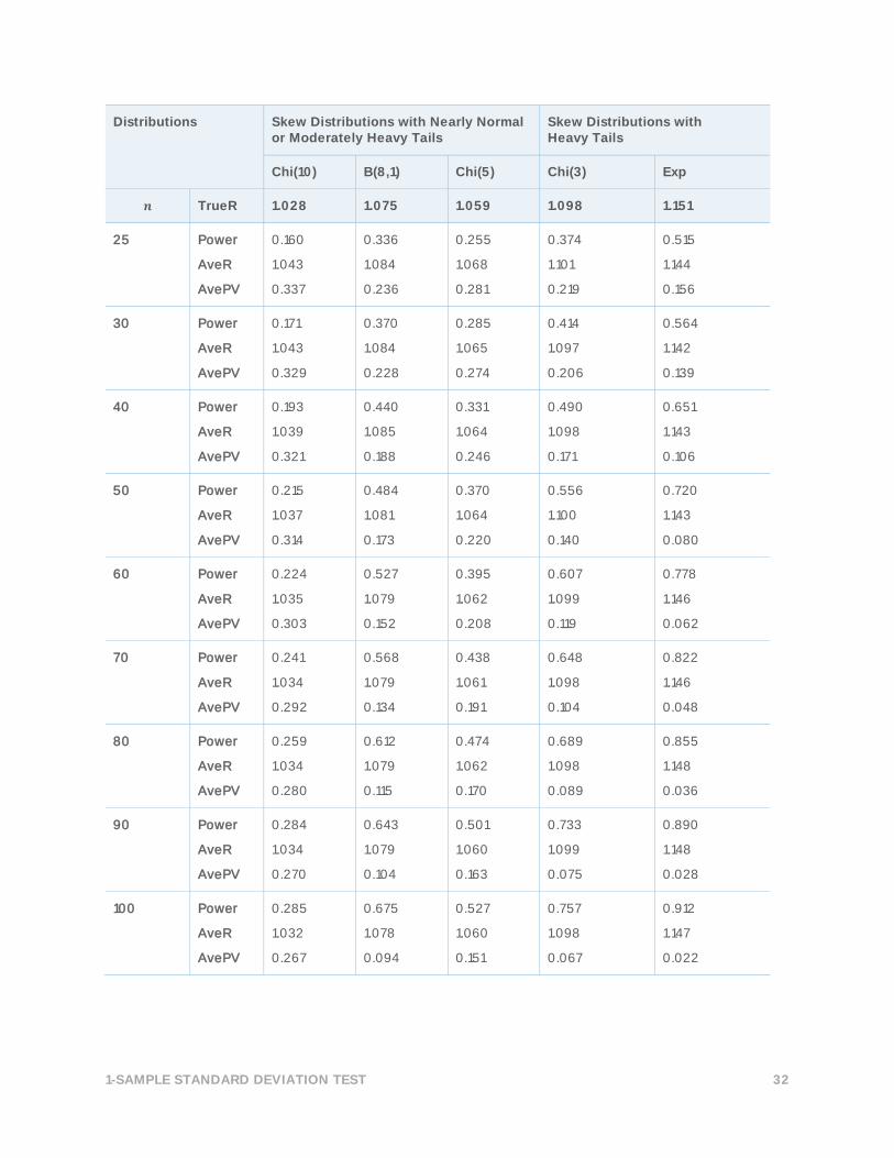
Table 6 Simulated power levels of the SJ test. The samples were generated from skew
distributions with nearly normal, moderately heavy, or heavy tails.
Distributions Skew Distributions with Nearly Normal or Moderately Heavy Tails
Skew Distributions with Heavy Tails
Chi(10) B(8,1) Chi(5) Chi(3) Exp
𝒏 TrueR 1.028 1.075 1.059 1.098 1.151
10 Power
AveR
AvePV
0.120
1.072
0.326
0.213
1.105
0.284
0.161
1.088
0.304
0.218
1.108
0.279
0.283
1.136
0.251
15 Power
AveR
AvePV
0.139
1.062
0.320
0.270
1.105
0.261
0.205
1.082
0.286
0.292
1.110
0.245
0.377
1.141
0.209
20 Power
AveR
AvePV
0.152
1.051
0.335
0.295
1.089
0.260
0.223
1.070
0.296
0.328
1.101
0.242
0.449
1.142
0.186
1-SAMPLE STANDARD DEVIATION TEST 32
Distributions Skew Distributions with Nearly Normal or Moderately Heavy Tails
Skew Distributions with Heavy Tails
Chi(10) B(8,1) Chi(5) Chi(3) Exp
𝒏 TrueR 1.028 1.075 1.059 1.098 1.151
25 Power
AveR
AvePV
0.160
1.043
0.337
0.336
1.084
0.236
0.255
1.068
0.281
0.374
1.101
0.219
0.515
1.144
0.156
30 Power
AveR
AvePV
0.171
1.043
0.329
0.370
1.084
0.228
0.285
1.065
0.274
0.414
1.097
0.206
0.564
1.142
0.139
40 Power
AveR
AvePV
0.193
1.039
0.321
0.440
1.085
0.188
0.331
1.064
0.246
0.490
1.098
0.171
0.651
1.143
0.106
50 Power
AveR
AvePV
0.215
1.037
0.314
0.484
1.081
0.173
0.370
1.064
0.220
0.556
1.100
0.140
0.720
1.143
0.080
60 Power
AveR
AvePV
0.224
1.035
0.303
0.527
1.079
0.152
0.395
1.062
0.208
0.607
1.099
0.119
0.778
1.146
0.062
70 Power
AveR
AvePV
0.241
1.034
0.292
0.568
1.079
0.134
0.438
1.061
0.191
0.648
1.098
0.104
0.822
1.146
0.048
80 Power
AveR
AvePV
0.259
1.034
0.280
0.612
1.079
0.115
0.474
1.062
0.170
0.689
1.098
0.089
0.855
1.148
0.036
90 Power
AveR
AvePV
0.284
1.034
0.270
0.643
1.079
0.104
0.501
1.060
0.163
0.733
1.099
0.075
0.890
1.148
0.028
100 Power
AveR
AvePV
0.285
1.032
0.267
0.675
1.078
0.094
0.527
1.060
0.151
0.757
1.098
0.067
0.912
1.147
0.022

1-SAMPLE STANDARD DEVIATION TEST 33
Distributions Skew Distributions with Nearly Normal or Moderately Heavy Tails
Skew Distributions with Heavy Tails
Chi(10) B(8,1) Chi(5) Chi(3) Exp
𝒏 TrueR 1.028 1.075 1.059 1.098 1.151
120 Power
AveR
AvePV
0.323
1.032
0.246
0.728
1.077
0.074
0.572
1.060
0.129
0.816
1.098
0.050
0.942
1.149
0.014
140 Power
AveR
AvePV
0.344
1.031
0.232
0.769
1.077
0.060
0.621
1.060
0.112
0.852
1.099
0.036
0.963
1.148
0.009
160 Power
AveR
AvePV
0.363
1.031
0.217
0.815
1.077
0.047
0.666
1.060
0.093
0.887
1.098
0.027
0.978
1.150
0.005
180 Power
AveR
AvePV
0.385
1.031
0.209
0.843
1.077
0.039
0.692
1.059
0.083
0.910
1.099
0.021
0.986
1.148
0.004
200 Power
AveR
AvePV
0.410
1.030
0.196
0.877
1.077
0.030
0.727
1.059
0.071
0.931
1.098
0.016
0.989
1.149
0.003
Our simulation results in Tables 5 and 6 are consistent with those published in Gel et al. (2007).
When the samples are from the normal populations, the simulated power levels (which in this
case represent the actual significance level of the test) are not far from the target level, even for
sample sizes as low as 25. When the samples are from heavy-tailed distributions, the power of
the test is low for small sample sizes but increases to at least 40% when the sample size reaches
40. Specifically, the power at sample size 40 is about 40.1% for the t-distribution with 5 degrees
of freedom, 66.5% for the Laplace distribution, and 65.1% for the exponential distribution.
For light-tailed distributions (the Beta(3,3) and the uniform distributions), the power of the test is
near 0 for small samples and decreases even further as the sample size increases. This is not
surprising because the evidence for these distributions actually supports the alternative
hypothesis of a lighter tailed distribution, rather than the alternative hypothesis of a heavier-
tailed distribution.
When the samples are from distributions with slightly heavier tails, such as the t-distribution
with 10 degrees of freedom or the chi-square distribution with 10 degrees of freedom, the
power levels are low for moderate to large sample sizes. For our purposes, this is actually a good
result because the test for one variance (standard deviation) performs well for these

1-SAMPLE STANDARD DEVIATION TEST 34
distributions and we do not want these distributions to be flagged as heavy-tailed. However, as
the sample size increases, the power of the test increases, so these slightly heavy-tailed
distributions are detected as heavy-tailed distributions.
Therefore, the rules for evaluating the tail weight of the distribution for this test must also take
into consideration the size of the sample. One approach for doing this is to calculate a
confidence interval for the measure of the tail weight; however, the distribution of the SJ statistic
is extremely sensitive to the parent distribution of the sample. An alternative approach is to
assess the heaviness of the tails of the distribution based on both the strength of the rejection
of the null hypothesis of the SJ test and the sample size. More specifically, smaller p-values
indicate heavier tails and larger p-values indicate lighter tails. However, larger samples tend to
have smaller p-values than smaller samples. Therefore, based on the simulated power levels,
sample sizes, and average p-values in Table 3, we devise a general set of rules for evaluating the
tails of a distribution for each sample using the SJ test.
For moderate to large sample sizes (40 ≤ 𝑛 ≤ 100), if the p-value is between 0.01 and 0.05, we
deem that there is mild evidence against the null hypothesis. That is, the distribution of the
sample is classified as a moderately heavy-tailed (M-type) distribution. On the other hand, if the
p-value is below 0.01, then there is strong evidence against the null hypothesis, and the parent
distribution of the sample is classified as a distribution with heavy tails (H-type).
For large samples (𝑛 > 100), we categorize the parent distribution as an M-type distribution if
the p-value falls between 0.005 and 0.01, and as an H-type distribution if the p-value is
extremely small (below 0.005). Note that when the sample size is below 40, the power of the SJ
test is generally too low for the distribution of the sample to be effectively determined.
The general classification rules for the validity of the 1-variance test using Bonett’s method are
summarized in Table 7 below.
Table 7 Classification rules for identifying the parent distribution of each sample (𝑝 is the p-
value of the SJ test)
Condition Distribution type
𝒏 < 40 None is determined
𝟏𝟎𝟎 ≥ 𝒏 ≥ 𝟒𝟎 and 𝒑 > 0.05 L-type distribution
𝒏 > 100 and 𝒑 > 0.01 L-type distribution
𝟒𝟎 ≤ 𝒏 ≤ 𝟏𝟎𝟎 and 𝟎. 𝟎𝟏 < 𝒑 ≤ 𝟎. 𝟎𝟓 M-type distribution
𝒏 > 100 and 𝟎. 𝟎𝟎𝟓 < 𝒑 ≤ 𝟎. 𝟎𝟏 M-type distribution
𝟒𝟎 ≤ 𝒏 ≤ 𝟏𝟎𝟎 and 𝒑 ≤ 𝟎. 𝟎𝟏 H-type distribution
𝒏 > 100 and 𝒑 ≤ 𝟎. 𝟎𝟎𝟓 H-type distribution

1-SAMPLE STANDARD DEVIATION TEST 35
As indicated earlier, based on the results of Tables 1 and 2 in simulation C1, the approximate
minimum sample size required to achieve a minimum of 0.93 coverage probability when
samples are generated from an L-type, an M-type, and an H-type distribution is 20, 80, and 200,
respectively. However, because the power of the SJ test is low for small samples, the minimum
sample size requirement for L-type distributions is set at 40.
Simulation F2: Verifying the rules for classifying distributions We generated samples from some of the distributions described in simulation C1 and used the
SJ test to determine the proportions of the samples that were classified in one of the three
distribution groups: L-type, M-type, and H-type. The simulation results are shown in Table 8.
Table 8 Fraction of 10,000 samples of different sizes from various distributions that are
identified as L-type, M-type, and H-type
𝒏 Distributions L-type M-type H-type
B(3,3) N(0,1) t(10) Chi(10) Chi(5) Lpl Exp
40 %L-type
%M-type
%H-type
99.6
0.4
0.0
94.0
5.5
0.5
81.5
14.0
4.5
80.3
14.0
5.7
66.6
20.0
13.4
33.0
31.9
35.1
34.4
22.9
42.8
50 %L-type
%M-type
%H-type
99.7
0.3
0.0
94.4
5.1
0.5
78.7
15.6
5.7
79.1
14.2
6.7
64.0
20.0
16.0
25.1
29.9
45.0
28.0
20.7
51.3
60 %L-type
%M-type
%H-type
99.7
0.3
0.0
94.5
5.1
0.5
77.3
16.4
6.3
77.3
15.0
7.7
59.1
22.0
18.9
18.5
27.4
54.1
22.6
19.2
58.2
70 %L-type
%M-type
%H-type
99.8
0.2
0.0
94.4
5.0
0.6
74.5
18.1
7.4
75.2
16.0
8.8
55.9
22.2
21.9
14.0
24.0
62.0
18.1
17.5
64.4
80 %L-type
%M-type
%H-type
99.9
0.1
0.0
94.3
5.1
0.6
74.1
17.8
8.2
74.4
16.7
8.9
53.0
22.8
24.2
10.0
21.0
69.0
13.9
15.5
70.6
90 %L-type
%M-type
%H-type
99.9
0.1
0.0
94.4
5.0
0.6
71.2
19.1
9.7
72.1
17.2
10.7
49.5
22.6
27.9
7.5
16.5
76.0
11.1
13.7
75.3

1-SAMPLE STANDARD DEVIATION TEST 36
𝒏 Distributions L-type M-type H-type
B(3,3) N(0,1) t(10) Chi(10) Chi(5) Lpl Exp
100 %L-type
%M-type
%H-type
99.9
0.1
0.0
94.5
4.9
0.6
70.8
19.5
9.7
70.3
17.9
11.8
47.3
22.7
30.0
4.8
14.3
80.9
8.9
11.8
79.4
120 %L-type
%M-type
%H-type
100.0
0.0
0.0
99.4
0.4
0.2
87.4
5.0
7.6
87.2
4.5
8.4
64.8
7.9
27.4
12.0
7.8
80.4
14.4
5.6
80.0
140 %L-type
%M-type
%H-type
100.0
0.0
0.0
99.3
0.5
0.2
86.0
5.2
8.8
85.1
5.0
9.9
60.5
8.6
30.9
7.0
5.6
87.4
9.9
4.1
86.0
160 %L-type
%M-type
%H-type
100.0
0.0
0.0
99.4
0.5
0.1
83.4
6.3
10.4
83.0
5.8
11.2
55.6
9.5
34.9
4.0
3.5
92.5
6.9
3.0
90.1
180 %L-type
%M-type
%H-type
100.0
0.0
0.0
99.3
0.5
0.2
81.1
6.8
12.1
81.7
5.9
12.4
51.0
9.4
39.6
2.5
1.9
95.6
4.6
2.2
93.2
200 %L-type
%M-type
%H-type
100.0
0.0
0.0
99.5
0.4
0.1
79.0
7.6
13.4
80.5
6.1
13.4
47.2
9.4
43.4
1.3
1.6
97.1
3.0
1.7
95.3
The results in Table 8 show that when samples are from light-tailed (L-type) and heavy-tailed
(H-type) distributions, a higher proportion of the samples are correctly classified. For example,
when samples of size 40 were generated from the Beta(3,3) distribution, 99.6% of the samples
were correctly classified as having lighter tails; when samples of size 90 were generated from the
Laplace distribution, 76.0% were correctly classified as having heavy tails. As a result, warning
messages in the Report Card regarding the validity of the test are not wrongly issued when
samples are truly from lighter tailed distributions, and are correctly issued when the sample
comes from a distribution with heavy tails and the minimum sample size requirement is not met.
In addition, for samples from distributions with moderately heavy tails (M-type), such as the chi-
square (5) distribution, a higher proportion of samples are misclassified as being light-tailed (L-
type) when the samples are small (for a sample size of 40, 66% of the samples are misclassified
as light-tailed distribution). Consequently, for these cases, warning messages in the Report Card
may not be issued even though the parent distributions have moderately heavy tails. However,
when the sample size is greater than 80, the misclassification as an L-type distribution has no
effect because the minimum sample size requirement has already been met.

1-SAMPLE STANDARD DEVIATION TEST 37

1-SAMPLE STANDARD DEVIATION TEST 38
© 2015, 2017 Minitab Inc. All rights reserved.
Minitab®, Quality. Analysis. Results.® and the Minitab® logo are all registered trademarks of Minitab,
Inc., in the United States and other countries. See minitab.com/legal/trademarks for more information.