1-s2.0-S0895717708000289-main

Mathematical and Computer Modelling 47 (2008) 1077–1088www.elsevier.com/locate/mcm

The amazing variety of motions of a loaded hoop

W.F.D. Theron∗, M.F. Maritz

Department of Applied Mathematics, University of Stellenbosch, Private Bag X1, Matieland, ZA7602, South Africa

Received 26 September 2006; received in revised form 11 June 2007; accepted 22 June 2007

Abstract

The subject of loaded hoops, and their ability to hop under certain conditions, received some attention at the turn of the century,inter alia by Tokieda, Pritchett and Theron. In this paper the emphasis is rather on extending the analysis of the motion before thehoop hops, including those cases where the hoop does not hop.

The results of numerical simulation based on a classical mechanical model of a loaded hoop is presented. Results show thatthe motion consists of an amazing variety of alternating phases of rolling and slipping, some of which may be absent. A list ofthirty-six possible sequences is included. Phase diagrams are presented to illustrate the relationship between the various slippingand rolling phases, as well as how they depend on the eccentricity, the friction coefficient and the initial angular velocity.c© 2008 Elsevier Ltd. All rights reserved.

Keywords: Classical mechanics; Rolling hoops; Eccentric hoops

1. Introduction

In this paper the two-dimensional dynamic behaviour of a loaded hoop is investigated, by which is meant a heavyrigid hoop to which a heavy particle is fixed on the rim.

The hypothetical problem of a loaded massless hoop rolling without slipping on a horizontal surface has been usedfor very many years as an interesting class-room problem for planar motion of rigid bodies, and was first publishedby J.E. Littlewood [1] in 1953 in “A Mathematician’s Miscellany”.

The same problem is considered by Tokieda [2], whose analysis is based on the geometric aspects of the motion.Both Littlewood and Tokieda conclude that the hoop will hop after rolling through 90◦ after starting from rest withthe particle at the highest point of its cycloidal path.

Subsequent papers by Butler [3] and Theron & du Plessis [4] considered the question of whether the masslesshoop could hop or not. The motion of real hoops, with mass and assumed to be rigid, were published by Pritchett [5],Theron [6] and Liu [7], also with some emphasis on the question of hopping.

Tokieda [2] reports having witnessed an experiment by Fred Almgren [8] in which a hula-hoop was loaded with abattery and hopped as predicted by Littlewood, namely that the hoop leaves the ground when the radius to the particleis approximately horizontal and the particle is moving downwards. Pritchett [5] also shows a stroboscopic photograph

∗ Corresponding author.E-mail addresses: [email protected] (W.F.D. Theron), [email protected] (M.F. Maritz).

0895-7177/$ - see front matter c© 2008 Elsevier Ltd. All rights reserved.doi:10.1016/j.mcm.2007.06.031

http://www.elsevier.com/locate/mcm

mailto:[email protected]

mailto:[email protected]

http://dx.doi.org/10.1016/j.mcm.2007.06.031

1078 W.F.D. Theron, M.F. Maritz / Mathematical and Computer Modelling 47 (2008) 1077–1088

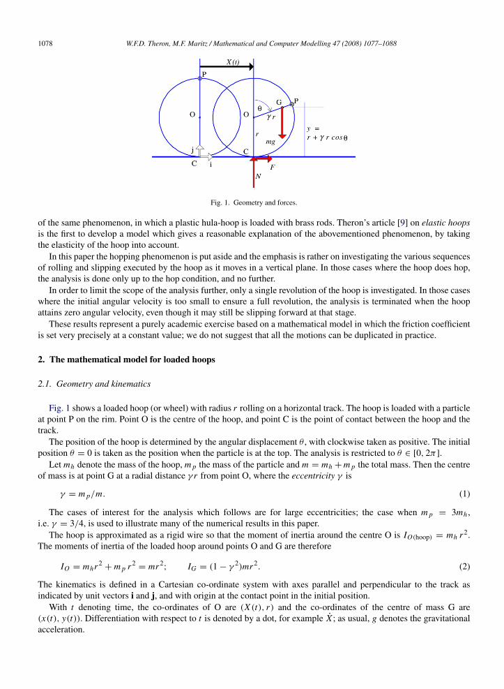
Fig. 1. Geometry and forces.

of the same phenomenon, in which a plastic hula-hoop is loaded with brass rods. Theron’s article [9] on elastic hoopsis the first to develop a model which gives a reasonable explanation of the abovementioned phenomenon, by takingthe elasticity of the hoop into account.

In this paper the hopping phenomenon is put aside and the emphasis is rather on investigating the various sequencesof rolling and slipping executed by the hoop as it moves in a vertical plane. In those cases where the hoop does hop,the analysis is done only up to the hop condition, and no further.

In order to limit the scope of the analysis further, only a single revolution of the hoop is investigated. In those caseswhere the initial angular velocity is too small to ensure a full revolution, the analysis is terminated when the hoopattains zero angular velocity, even though it may still be slipping forward at that stage.

These results represent a purely academic exercise based on a mathematical model in which the friction coefficientis set very precisely at a constant value; we do not suggest that all the motions can be duplicated in practice.

2. The mathematical model for loaded hoops

2.1. Geometry and kinematics

Fig. 1 shows a loaded hoop (or wheel) with radius r rolling on a horizontal track. The hoop is loaded with a particleat point P on the rim. Point O is the centre of the hoop, and point C is the point of contact between the hoop and thetrack.

The position of the hoop is determined by the angular displacement θ , with clockwise taken as positive. The initialposition θ = 0 is taken as the position when the particle is at the top. The analysis is restricted to θ ∈ [0, 2π ].

Let mh denote the mass of the hoop, m p the mass of the particle and m = mh + m p the total mass. Then the centreof mass is at point G at a radial distance γ r from point O, where the eccentricity γ is

γ = m p/m. (1)

The cases of interest for the analysis which follows are for large eccentricities; the case when m p = 3mh ,i.e. γ = 3/4, is used to illustrate many of the numerical results in this paper.

The hoop is approximated as a rigid wire so that the moment of inertia around the centre O is IO(hoop) = mh r2.The moments of inertia of the loaded hoop around points O and G are therefore

IO = mhr2+ m p r2

= mr2; IG = (1 − γ 2)mr2. (2)

The kinematics is defined in a Cartesian co-ordinate system with axes parallel and perpendicular to the track asindicated by unit vectors i and j, and with origin at the contact point in the initial position.

With t denoting time, the co-ordinates of O are (X (t), r) and the co-ordinates of the centre of mass G are(x(t), y(t)). Differentiation with respect to t is denoted by a dot, for example X ; as usual, g denotes the gravitationalacceleration.

W.F.D. Theron, M.F. Maritz / Mathematical and Computer Modelling 47 (2008) 1077–1088 1079

A rigid hoop in contact with the surface has two degrees of freedom, which are here selected as X and θ . Then thefollowing constraints on x(t) and y(t) are introduced :

x(t) = X (t) + γ r sin θ(t), y(t) = r + γ r cos θ(t). (3)

One of the fundamental motions of the hoop is rolling, characterised by the constraint that the contact point C ismomentarily at rest; i.e. that

X − r θ = 0. (4)

We assume that the motion commences at t = 0 from an initial position defined by θ(0) = 0, X (0) = 0, and thatX(0) = r θ (0) to ensure rolling from the start.

It is convenient to define non-dimensional velocities and accelerations as follows:

α = (r/g)θ; ω =√

(r/g) θ; ω0 =√

(r/g) θ(0); Vx = X/√

rg. (5)

2.2. Kinetics

The kinetics of the problem is defined in terms of the three forces shown in Fig. 1, namely the weight mg, thenormal reaction N , and the horizontal friction force F . Newton’s second law determines the relationship between theforces and the accelerations.

Taking components in the horizontal direction, F = mx , or differentiating (3) and using (5),

F = mg(X/g + γα cos θ − γω2 sin θ). (6)

Taking components perpendicular to the plane, N − mg = my, or,

N = mg(1 − γα sin θ − γω2 cos θ). (7)

Taking clockwise moments about the centre of mass, Nγ r sin θ − Fy = IG θ . Dividing by mgr and using (2) and(5),

(N/mg)γ sin θ − (F/mg)(y/r) = (1 − γ 2)α. (8)

The maximum value of the friction force places a constraint on the forces. Denoting the coefficient of friction byµ,1 Coulomb’s law states that

|F | ≤ µN . (9)

The total energy of the system is the sum of the potential and kinetic energies, and is given by

E = mgr(1 + γ cos θ) +12

m(X + γ r θ cos θ)2+

12

m(−γ r θ sin θ)2+

12

IG θ2.

While the hoop is rolling, using (2), (4) and (5), this simplifies to

Er = mgr(1 + ω2)(1 + γ cos θ). (10)

2.3. Rolling

As stated earlier, the initial conditions are always selected so as to ensure rolling motion to start with. The simplestmethod of obtaining the solution for rolling motion is to equate the total energy with the energy at the beginning ofthe roll. Using (10), and denoting the point where rolling starts as θr and ωr = ω(θr ),

ω2=

((1 + ω2

r )(1 + γ cos θr )/(1 + γ cos θ))

− 1. (11)

1 To simplify the analysis, no distinction is made between static and kinetic friction coefficients.


Note that for the first rolling phase, θr = 0; for the subsequent rolling phases θr is the position where slipping ends.From (4) and (5), X/g = α; using this with (6) and (7) in (8)

α =12γ sin θ(1 + ω2)/(1 + γ cos θ). (12)

The reaction forces can now be calculated from (6) and (7). Substituting (12) in (6), the expression for F simplifiesto

F/mg =12γ sin θ(1 − ω2). (13)

This clearly implies that for θ < π , F > 0 while ω < 1, and vice versa; also that the initial value F(0) = 0.Furthermore, from (7), the initial value of the normal reaction is N (0) = mg(1 − γω2

0). Defining the critical initialvelocity, ω0, as

ω0 =√

(1/γ ), (14)

this implies that for the initial normal reaction to be positive, the initial angular velocity must be less than this criticalvalue. Consequently, the hoop will hop immediately if ω0 > ω0.

A transition from rolling to slipping occurs at the point where |F | = µN , unless one of the final conditions atposition θF , to be defined later, is reached.

2.4. Spinning and skidding

Assume that the hoop rolls until the angular displacement is θs when slipping commences with N (θs) > 0 and|F(θs)| = µN (θs). The initial conditions for the slipping motion are defined by Xs = r θs and ωs = ω(θs).

The two possibilities for the orientation of the friction force need to be considered separately. The hoop is said tobe spinning if F = +µN i, with r θ > X . Similarly, motion is defined as skidding if the friction force is negative,F = −µN i, with r θ < X .

The two cases are handled by one set of equations by introducing a slip factor S, where S = γ sin θ−µ(1+γ cos θ)

for spinning, and S = γ sin θ + µ(1 + γ cos θ) for skidding.Using (3) and (7), the torque equation (8) now simplifies to

α =S(1 − γ cos θω2)

1 − γ 2 + Sγ sin θ. (15)

Noting that (5) implies that dω2

dθ= 2α, this can be written as the first-order differential equation

dω2

dθ=

2S(1 − γ cos θω2)

1 − γ 2 + Sγ sin θ. (16)

No analytical solution could be found for (16), and this equation is integrated numerically with the initial conditionω(θs) = ωs , using a fourth-order Runge–Kutta method.

With ω2 known at a specific position, α is calculated from (15). The normal reaction N is obtained from (7), andthe friction force F is obtained from Coulomb’s law. Eq. (6) is now used to calculate the value of X , and X is obtainedby numerical integration.

The slipping motion described by this solution will change to rolling when X(θr ) = r θ (θr ). If this does not happen,the motion stops with one of the final conditions at position θF .

2.5. Final conditions

The analysis of the sequence of alternating rolling and slipping phases ends with a final condition at a positiondenoted by θF ; this final condition can be either θF = 2π , implying that a complete revolution has been completed;or NF = N (θF ) = 0, i.e. the normal reaction becomes zero and the hoop hops; or ωF = ω(θF ) = 0, i.e. the hoopstops rotating momentarily before starting to rotate backwards. Note that ωF = 0 does not imply that X is also zero.


(a) Ratio of F/N . (b) Reaction forces.

(c) Kinematic quantities.

Fig. 2. Detailed results for a typical example of a rigid hoop, using γ = 3/4, µ = 0.4 and ω0 = 0.5.

3. Numerical results

The behaviour of the hoop depends on the values of the eccentricity γ , the friction coefficient µ and the initialvelocity as defined by ω0.

The numerical results in this and the following sections were obtained by implementing the algorithm implied bySections 2.3–2.5, using the ODE45-function of MATLAB [10] for the numerical integration.

3.1. A typical example

In this section the results of a typical example are given. Taking a particle mass three times the hoop mass so thatγ = 3/4, together with µ = 0.4 and an initial velocity of ω0 = 0.5, the results shown in Fig. 2 are obtained.

The solid curve in Fig. 2(a) shows the ratio F/N as a function of θ , where F and N are calculated as described inSections 2.3 and 2.4. This graph provides a very clear description of the motion. The first maximum value is less thanthe friction coefficient of µ = 0.4, which value is indicated by the horizontal dashed line. The hoop therefore rolls to


the position where F/N = −µ and it starts skidding. This is followed by rolling, a spinning phase where F/N = µ

and a final rolling phase all the way to the top, where the analysis ends with θF = 360◦.Fig. 2(b) shows graphs of the normal reaction and friction force, normalised with respect to the weight mg. The

normal reaction is plotted for scaled values µN/mg, and the region of spinning where F = µN is therefore clearlyrecognisable. The normal reaction is essentially symmetric with a maximum value at θ = 180◦; the friction force isessentially skew-symmetric with zero values at θ = 0◦

; 180◦; 360◦. The normal reaction is clearly still positive at the

end of the graph; therefore hopping does not occur in this case.Graphs of the kinematic quantities are shown in Fig. 2(c), as labelled. The angular velocity ω is shown as a solid

curve, and the velocity, Vx , of point O as a dotted curve; at this scale the two graphs are practically identical, althoughthe values do differ slightly during the short skidding and spinning phases when ω < Vx and ω > Vx respectively.This is shown more clearly by the dash-dotted curve showing the difference (ω − Vx ), magnified by a factor of ten.The graph also shows that the angular velocity is still positive when the particle reaches the top.

The graph of the angular acceleration α is essentially skew-symmetric, being positive while θ < 180◦ and theparticle is moving downwards and therefore providing a positive torque around the contact point, and being negativewhen θ > 180◦ and the particle is moving upwards.

The angular velocity clearly reaches a maximum value at θ = 180◦, where the angular acceleration changes frompositive to negative.

3.2. The rolling curve

In Fig. 2(a) an additional dotted curve shows the F/N -ratio for rolling; i.e. the curve that would have applied if thehoop had not started to slip; this curve will be referred to as the rolling curve. The rolling curve is clearly independentof the friction coefficient, and is fundamental to understanding many of the aspects of the behaviour of the hoop.

The rolling curve is available in analytic form from (13) and (7). All the results shown here were however obtainedby direct numerical calculation, using (7) and (11) to (13).

As clearly seen in Fig. 2(a), the rolling curve has four extrema; as long as these extreme values remain inside thehorizontal band bounded by −µ and +µ, the hoop will roll through to 360◦. Slipping occurs only where the rollingcurve leaves this horizontal band.

The four extrema occur in pairs, with the first maximum and second minimum being the same magnitude, and soalso the two middle extrema. We find it useful for later classification to define the first two extrema as critical valuesof the friction coefficient, as follows :

µL = max(F/N ); µH = | min(F/N )|; θ < 180◦. (17)

The subscripts refer to L¯ight and H

¯eavy friction respectively; the implications will be discussed later.

The effect of different initial velocities is shown in Fig. 3. Keeping γ = 3/4 in Fig. 3(a), it is seen that increasingω0 causes a decrease in µL and an increase in µH . With this eccentricity, µL < µH for all ω0. For ω0 effectively zero(using ω0 = 0.001), µH = 0.377 is shown by the dashed horizontal lines.

Also shown is the case in Fig. 2(a), shown by the curve labelled 0.5, and curves labelled 0.7 and 1. For ω0 = 1,µL = 0 at θ = 0 and it can be shown that µH → ∞.

The effect of decreasing the eccentricity is shown in Fig. 3(b), for the case γ = 2/3. For this eccentricity there arethree possibilities:

(1) µL > µH for small initial velocities, e.g. ω0 = 0;(2) µL = µH = 0.257 for ω0 = 0.317;(3) µL < µH for ω0 > 0.317, e.g. ω0 = 0.7 and 1. The curve for ω0 = 1 again shows that µL = 0, as can be derived

from (13).

A notable feature in the graphs in Fig. 2 is the discontinuity in the forces and angular acceleration at the pointswhere the slipping motion changes back to rolling. This is similar to the discontinuity of magnitude µ in F and α

found when a concentric hoop starts rolling after slipping. With loaded hoops the F/N -curve drops back to the rollingcurve for the next rolling phase, and the magnitude of the discontinuities can vary from almost zero to 2µ. In anyslipping phase there is a loss of energy; consequently the rolling curve after a slipping phase is slightly different tothe one before. However, the difference between the two rolling curves is not discernable in this example at the scalebeing used.


(a) γ = 3/4.

(b) γ = 2/3.

Fig. 3. First half of the rolling curves for different γ and ω0.

3.3. Phases of the motion

In the example shown in Fig. 2 the hoop experiences five phases before it reaches the top, i.e. roll-skid-roll-spin-roll. These phases originate from the fact that the rolling curve as shown in Fig. 2(a) exceeds the horizontal bandbetween −µ and +µ at two places, resulting in the skidding and spinning phases. In addition these two slippingphases were interspersed by three rolling phases. It can be seen that the most complete phase sequence consists of thenine phases roll-spin-roll-skid-roll-spin-roll-skid-roll, occurring when the rolling curve exceeds the domain between−µ and +µ in the vicinity of all four of its extrema.

In order to facilitate the classification of the motion, the following labels will be used: R for Roll (|F | ≤ µN ); Sfor Spin (F = +µN ); and D for skiD (F = −µN ). Hyphens will be used as place holders where needed to show theabsence of a particular phase.

The final conditions are labelled as Z for Zero angular velocity (ωF = 0); T for reaching the Top (θF = 2π ), and Hfor Hop (NF = 0). A space separates the final label from the rest.

Using this labeling scheme, the example above is labelled RDRSR-- T, implying that the final skid and roll aremissing. Another example is RS-DRS-D- Z, implying that three rolling phases are missed and that the analysis endswith zero angular velocity before the particle has reached the top.


The * stands for a ‘wild card’ and indicates any phase sequence or final condition. Note that the sequence *S-D*occurs at the end of a spinning phase when the discontinuity in the F/N -diagram is limited to 2µ and the spin changesto skid without an intermediate rolling phase. A similar situation is found for an instantaneous change from skid tospin, labelled *D-S*.

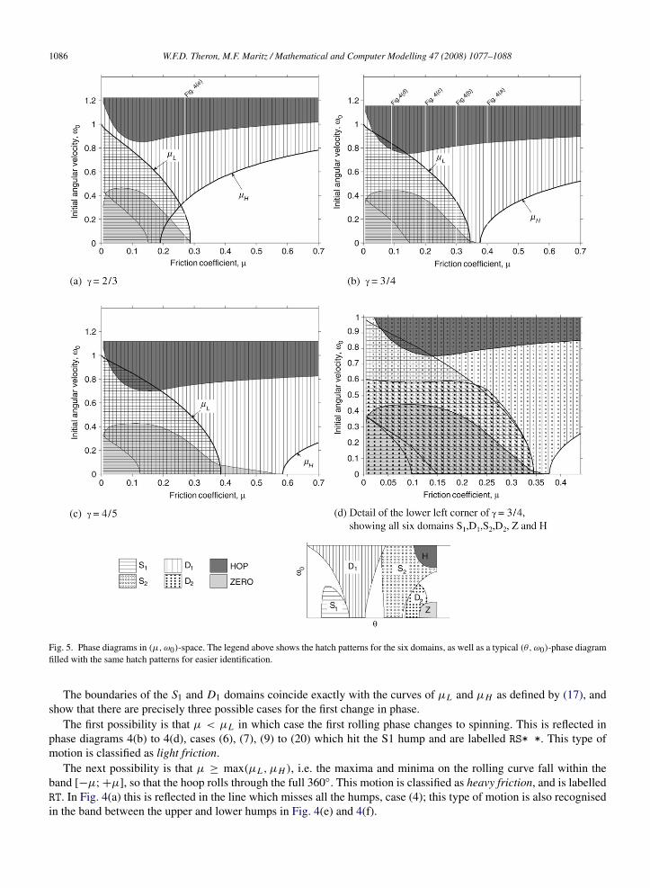
4. Phase diagrams

Numerical experimentation shows that an amazing number of combinations of phases are possible. In order tocomprehend the full scope of this variety, we make use of two types of phase diagram.

4.1. Phase diagrams in (θ, ω0)-space

Firstly, phase diagrams in the (θ, ω0)-space can be drawn, each for a fixed (γ, µ) parameter pair. Six of these areshown in Fig. 4; note that the first four are for the same eccentricity with decreasing friction.

Each diagram is obtained by calculating the numerical solution for a range of ω0-values. For each solution thevalues of θ where the phase changes are recorded, and these points are plotted on the (θ, ω0)-plane. The points of asingle motion therefore lie on a horizontal line at vertical ordinate ω0. It becomes clear that these points describe theboundaries of domains in the (θ, ω0)-plane for each of the possible phases. Besides the interspersing rolling phases,there are four slipping phases, viz. first spinning phase, the first skidding phase, second spinning phase, and secondskidding phase.

The domains in which spinning occurs are labelled S1 and S2 respectively and are filled with light grey, and thedomains where skidding occurs are labelled D1 and D2 respectively and are filled with dark grey. The domains whererolling occurs are unlabelled and filled with a diagonal hatch pattern.

The phases S1 and D2 form a pair and rise as hump shapes from the bottom of the diagram with decreasing µ.Their maxima have the same value (e.g. Fig. 4(b)) except in those cases where the point where the maximum wouldhave been is obscured by an earlier phase (e.g. Fig. 4(d)). Similarly D1 and S2 form a pair and drop down from the topwith decreasing µ and their minima have the same value (e.g. Fig. 4(a)) except when obscuration by an earlier phaseprevents this (e.g. Fig. 4(d)).

It is also useful to show the final condition of the motion. The points (θF , ω0) form curves at the right handboundary of the (θ, ω0)-plane, viz. the Zero curve, labelled Z, for lower values of ω0; the Top line, which is a verticalline at θ = 360◦; and the Hop curve, labelled H, for higher values of ω0.

The domain of motion is bounded at the top by the horizontal line ω0 = ω0, from (14).In each diagram the pattern for a particular value of ω0 may be obtained by following a horizontal line from left to

right and noting the domains through which this line passes.For example the case described in Section 3.1 is indicated in Fig. 4(a), case (3), by a horizontal line at ω0 = 0.5;

the label RDRSR-- T is easily recognised.A region where two humps overlap corresponds to cases where the discontinuity in F/N needs to be limited to 2µ,

thereby eliminating the intermediate rolling phase. Cases (13)–(20) in Fig. 4(d) all illustrate this phenomenon.A total of twenty-five different patterns are shown on the six diagrams in Fig. 4. Fig. 4(d) is remarkable in that ten

different patterns, of which only the eight new ones are shown, are found for this single (γ, µ) pair.Fig. 4(e) and 4(f) are for smaller eccentricities and show five new patterns. In these cases there is always a clear

gap between the upper and lower humps.

4.2. Phase diagrams in (µ, ω0)-space

A second type of phase diagram, providing a more synoptic view of the various possible phases, is shown in Fig. 5.Here the (µ, ω0)-space for a fixed value of γ is used, showing the domains where a particular slipping phase occursbut suppressing the information about the rolling phases and the interval of θ for each particular phase.

In order to avoid cluttering the diagram, it was decided to include only the phases S1 and D1, as well as the domainswhere Hop and Zero occur, in Fig. 5(a)–(c). Fig. 5(d) is an enlargement of the lower left corner of Fig. 5(b), showingall four slipping phases.

Fig. 5 was produced by numerically computing the maximum of S1 as well as the minimum of D1, both as functionsof µ for a fixed value of γ . The minimum of the Hop curve and the maximum of the Zero curve were similarly


(a) γ = 3/4, µ = 0.4. (b) γ = 3/4, µ = 0.3.

(c) γ = 3/4, µ = 0.2. (d) γ = 3/4, µ = 0.09.

(e) γ = 2/3, µ = 0.27. (f) γ = 1/4, µ = 0.05.

Fig. 4. Phase diagrams in (θ, ω0)-space.

computed numerically. The domains overlap significantly in the phase diagram, and hatching fill patterns were usedin order to allow overlap of various domains to be recognised.

All the domains present at any coordinate (µ, ω0) in this diagram indicate the slipping phases that will be present,as well as the final condition that will be encountered.


Fig. 5. Phase diagrams in (µ, ω0)-space. The legend above shows the hatch patterns for the six domains, as well as a typical (θ, ω0)-phase diagramfilled with the same hatch patterns for easier identification.

The boundaries of the S1 and D1 domains coincide exactly with the curves of µL and µH as defined by (17), andshow that there are precisely three possible cases for the first change in phase.

The first possibility is that µ < µL in which case the first rolling phase changes to spinning. This is reflected inphase diagrams 4(b) to 4(d), cases (6), (7), (9) to (20) which hit the S1 hump and are labelled RS* *. This type ofmotion is classified as light friction.

The next possibility is that µ ≥ max(µL , µH ), i.e. the maxima and minima on the rolling curve fall within theband [−µ; +µ], so that the hoop rolls through the full 360◦. This motion is classified as heavy friction, and is labelledRT. In Fig. 4(a) this is reflected in the line which misses all the humps, case (4); this type of motion is also recognisedin the band between the upper and lower humps in Fig. 4(e) and 4(f).


Owing to the symmetry of the rolling curve, the only other possibility is that shown in Fig. 2(a), namely thatµL < µ < µH . In this case the hoop stops rolling and starts skidding when F = −µ N . This is reflected in, forexample, phase diagram 4(a) for cases (1)–(3) which hit the D1 hump first. This is classified as medium friction andis labelled RD* *.

Fig. 5(a)–(c) illustrate the effect of increasing the eccentricity. Inter alia, the region of heavy friction decreasesdrastically as the eccentricity increases, with a corresponding, but smaller, increase in the region of light friction.

Any vertical line of constant µ in Fig. 5 corresponds to a (θ, ω0)-phase diagram such as, for example, Fig. 4(a). Apoint in Fig. 5 corresponds to one specific example; e.g., point (0.4, 0.5) in Fig. 5(d) is the typical example shownin Fig. 2, hitting the D1 and S2 domains. The line ω0 = ω0, from (14), again defines the upper limit for the initialvelocity. The figures also reflect the earlier finding that µL = 0 when ω0 = 1.

Note the small sub-region of medium friction immediately above and to the right of point (0.25, 0.5) in Fig. 5(d).This includes the D1, S2 and D2 regions, which is unusual in that the S1 region is missed but the D2 region is hit. Thefull pattern for points in this region can be shown to be RDRS-DR T. This is not found on any of the phase diagramsin Fig. 4, and is listed as pattern nr. 3 in Table 1.

5. List of possible motions

Table 1 contains a list of thirty-six possible motions; this includes the twenty-five patterns shown in Fig. 4 pluseleven more found for other parameters. Only one value of γ and µ is given for each motion; clearly many more arepossible. In each case the corresponding range of initial velocities is given, with the lowest and highest values of ω0shown in column 6. Column 7 refers to the phase diagrams in Fig. 4.

The patterns for heavy, medium and light friction are listed separately, and labelled as type HF, MF and LFrespectively. The medium and light friction patterns are sorted according to the number of missing phases. The lightfriction cases are also separated into two sub-classes based on the first three phases, namely cases labelled RSR* *,and those labelled RS-* *. The last mentioned includes all the cases where the S1 and D1 domains overlap, and onlyoccurs for small friction coefficients and low initial velocities.

In some of the more unusual cases the range of initial velocities is unrealistically small and precise, as for examplepatterns nr. 19, 25, 27 and 33. Owing to this, we do not claim to have found all possible motions; there may still be afew hiding out there!

6. Conclusions

An observer of an actual loaded hoop in motion may notice that it performs both slipping and rolling. However,the motion is usually too fast for the average observer to differentiate between all the different phases, and thereforethe variety of possible sequences is not noticed and consequently not appreciated.

It is only in performing numerical simulations that the somewhat bewildering variety of sequences becomesapparent. The existence of various alternating phases of rolling and slipping is known from [5,6]. It soon becomesclear however that performing only a few numerical simulations and the use of only a few parameter sets cannot revealthe broad picture. We believe that the use of numerically calculated phase diagrams as presented in this paper, as wellas the introduction of the ‘rolling curve’ for interpreting the origin and behaviour of the phase domains, significantlyclarify and illuminate the behaviour of a loaded hoop.

It must be understood that these results represent a purely academic exercise based on a mathematical model inwhich the friction coefficient is set very precisely at a constant value; this situation can clearly not be duplicated ina practical experiment. However, high speed photography of actual loaded hoops ought to display the four slippingphases interspersed by rolling phases. It could be expected that the phase domains may be distorted and the domainboundaries be somewhat fuzzy due to the incapability of maintaining a constant friction coefficient in the experimentalsetup. Also, the difference in kinetic and static friction coefficients, conveniently ignored in our simulations, mayfurther perturb the domain boundaries.

The thirty-six different patterns listed in Table 1 constitute what we consider to be an amazing number of differentmotions of a loaded rigid hoop. Our analysis is restricted to initial conditions enforcing rolling as the first phase, anda final condition as defined in Section 2.5. If these restrictions were to be lifted to allow for other initial conditionsand for analysis for θ > 2π and for ω < 0, an even greater variety of motions will occur.


Table 1List of patterns

Type Ref. Pattern γ µ ω0-range Phase dgm

HF 1 R T 3/4 0.4 (0 ; 0.15 ] 4a(4)

MF 2 RDRSRDR T 3/4 0.3 [0.35; 0.36] 4b(5)3 RDRS-DR T 3/4 0.24 [0.54; 0.55]4 RDRSR-- T 3/4 0.4 [0.16; 0.80] 4a(3)5 RDRSR-- Z 4/5 0.4 (0; 0.06]6 RDRS--- H 3/4 0.4 [0.85; 1.15] 4a(1)7 RDRS--- T 3/4 0.4 [0.81; 0.84] 4a(2)8 RD-SR-- T 2/3 0.15 [0.70; 0.72]9 RD-S--- H 3/4 0.2 [0.82; 1.15] 4c(8)

10 RD-S--- T 1/4 0.05 [1.07; 1.87] 4f(23)

LF 11 RSRDRSRDR T 3/4 0.3 [0.13; 0.34] 4b(6)12 RSRDRSRDR Z 3/4 0.3 (0; 0.12] 4b(7)13 RSRDRSRD- T 1/2 0.09 [0.46; 0.52]14 RSRDRSRD- Z 2/3 0.2 [0.11; 0.24]15 RSRDRSR-- T 3/4 0.2 [0.59; 0.63] 4c(9)16 RSRDRS-DR T 3/4 0.2 [0.49; 0.58] 4c(10)17 RSRDRS--- T 4/5 0.2 [0.66; 0.68]18 RSRD-S--- H 3/4 0.09 [0.79; 0.84] 4d(13)19 RSRD-S--- T 3/4 0.1 0.7720 RSR--S-D- Z 3/4 0.09 [0.10; 0.19] 4d(19)21 RSR----DR T 2/3 0.27 [0.06; 0.24] 4e(21)22 RSR----DR Z 2/3 0.27 (0; 0.05] 4e(22)23 RSR----D- T 1/4 0.05 [0.32; 0.49] 4f(24)24 RSR----D- Z 1/4 0.05 [0.17; 0.31] 4f(25)25 RS-DRSRDR Z 3/4 0.24 0.2726 RS-DRSRD- Z 3/4 0.24 [0; 0.26]27 RS-DRS-DR Z 3/4 0.24 0.2828 RS-DRS-DR T 3/4 0.2 [0.37; 0.48] 4c(11)29 RS-DRS-D- Z 3/4 0.2 (0; 0.36] 4c(12)30 RS-D-S--- T 3/4 0.09 [0.64; 0.78] 4d(14)31 RS-D-SR-- T 3/4 0.09 [0.59; 0.63] 4d(15)32 RS-D-S-DR T 3/4 0.09 [0.50; 0.58] 4d(16)33 RS-D-S-DR Z 3/4 0.1 0.4426634 RS-D-S-D- T 3/4 0.09 [0.45; 0.49] 4d(17)35 RS-D-S-D- Z 3/4 0.09 [0.39; 0.44] 4d(18)36 RS-----D- Z 3/4 0.09 (0; 0.09] 4d(20)

References

[1] J.E. Littlewood, Littlewood’s Miscellany, Cambridge University Press, 1986.[2] T.F. Tokieda, The hopping hoop, Am. Math. Monthly 104 (1997) 152–153.[3] J.P. Butler, Hopping hoops don’t hop, Am. Math. Monthly 106 (1999) 565–568.[4] W.F.D. Theron, N.M. du Plessis, The dynamics of a massless hoop, Am. J. Phys. 69 (2001) 354–359.[5] T. Pritchett, The hopping hoop revisited, Am. Math. Monthly 106 (1999) 609–617.[6] W.F.D. Theron, The rolling motion of an eccentrically loaded wheel, Am. J. Phys. 68 (2000) 812–820.[7] Y.Z. Liu, Y. Xue, Qualitative analysis of a rolling hoop with mass unbalance, Acta Mech. Sinica 20 (2004) 672–675.[8] D. Mackenzie, Fred Almgren (1933–1997), Notices Am. Math. Society 44 (1997) 1102–1106.[9] W.F.D. Theron, The dynamics of an elastic hopping hoop, Math. Comput. Modelling 35 (2002) 1135–1147.

[10] MATLAB, The Mathworks, Inc., 3 Apple Hill Drive, Natick, Massachusets 01760-2098.

Documents

1-s2.0-S0895717708000289-main