PS

Ya

b

1

ItNateTwtba((rflo

nsFtg

0h

chemical engineering research and design 9 1 ( 2 0 1 3 ) 1085–1094

Contents lists available at SciVerse ScienceDirect

Chemical Engineering Research and Design

j ourna l h omepage: www.elsev ier .com/ locate /cherd

attern matching of alarm flood sequences by a modifiedmith–Waterman algorithm

ue Chenga,∗, Iman Izadib, Tongwen Chena

Department of Electrical and Computer Engineering, University of Alberta, Edmonton T6G 2V4, CanadaMatrikon Inc., Edmonton T5J 3N4, Canada

a b s t r a c t

Alarm flooding is one of the main problems in alarm management. Alarm flood pattern analysis is helpful for root

cause analysis of historical floods and for incoming flood prediction. This paper deals with a data driven method

for alarm flood pattern matching. An alarm flood is represented by a time-stamped alarm sequence. A modified

Smith–Waterman algorithm considering the time stamp information is proposed to calculate a similarity index of

alarm floods. The effectiveness of the algorithm is validated by a case study on actual chemical process alarm data.

© 2012 The Institution of Chemical Engineers. Published by Elsevier B.V. All rights reserved.

Keywords: Alarm flood; Time-stamped sequences; Approximate sequence matching; Smith–Waterman algorithm;

Knowledge extraction

sequence patterns can be identified manually. Some structural

. Introduction

n large industrial plants, alarm systems are of great impor-ance to meet the demand of safety, quality and efficiency.owadays, hardware and software advances make it easy toccess almost every process variable that can be measured;his provides alarm systems more process information. How-ver, a serious problem exists in the industry: alarm flooding.ens or hundreds of alarms may arise during a short period,hich can overwhelm even experienced operators. Opera-

ors cannot analyze every alarm properly during alarm floodsecause of shortage of time; so they can only acknowledge thelarms and handle the abnormality based on their experienceFolmer et al., 2011). As a result, EEMUA and ISA standardsEEMUA, 2007; ISA, 2009) suggest that an operator should noteceive more than six alarms per hour, and define an alarmood as the period of more than 10 alarms per 10 min perperator.

It is shown in Henningsen and Kemmerer (1995) that a largeumber of unimportant alarms fall within three categories:tanding alarms, repetitive alarms, and consequence alarms.or standing and repetitive alarms, such widely implementedechniques as delay-timer, deadband and shelving are sug-

ested in EEMUA (2007) and ISA (2009). An intelligent alarm

∗ Corresponding author.E-mail addresses: cheng5@ualberta.ca (Y. Cheng), iman.izadi@matrReceived 26 July 2012; Received in revised form 21 October 2012; Acce

263-8762/$ – see front matter © 2012 The Institution of Chemical Engittp://dx.doi.org/10.1016/j.cherd.2012.11.001

management software focusing on chattering and standingalarms was developed and successfully implemented on arefinery process (Liu et al., 2003; Srinivasan et al., 2004). Duringsteady operating conditions, the alarm rate can be effectivelyreduced to a manageable level thanks to these techniques. Inabnormal situations, however, it is still very difficult to get ridof alarm floods though these techniques can suppress someof the alarms. The remaining alarms are mainly consequencealarms. Compared with standing and repetitive alarms, con-sequence alarms are more complicated and more difficultto handle. Consequence alarms are mainly caused by abnor-mality propagation. Usually at the beginning of an abnormalsituation, a few alarms arise, followed by many cascadedalarms, which eventually lead to an alarm flood. As a result, ifthe correlations among different alarms can be obtained, theinformation will be helpful to handle consequence alarms.

1.1. State of the art concerning alarm sequencepattern analysis

The most accurate approaches for alarm sequence patternanalysis are process knowledge based methods. The alarm

ikon.com (I. Izadi), tchen@ualberta.ca (T. Chen).pted 1 November 2012

modeling tools such as signed digraphs (SDG) are helpful for

neers. Published by Elsevier B.V. All rights reserved.

1086 chemical engineering research and design 9 1 ( 2 0 1 3 ) 1085–1094

abnormality propagation path searching and hence for identi-fying alarm sequence patterns (Umeda et al., 1980). However,these knowledge based methods are usually very time con-suming to implement and require involvement of experts.

To reduce the analysis time, data mining techniques area good choice. Pioneer work on applying sequential patternmining to consequence alarm suppression includes Cisar et al.(2009), Hostalkova and Stluka (2010), Folmer et al. (2011),and Folmer and Vogel-Heuser (2012). In Cisar et al. (2009)and Hostalkova and Stluka (2010), the authors modified theGeneralized Sequential Patterns (GSP) algorithm (Srikant andAgrawal, 1996) to search for frequent alarm sequences (pat-terns) in the historical alarm records. They emphasized thatbesides the chronological order the triggering time was alsovery important, so time stamps of alarms were consideredto add time constraints in their algorithm. They also pointedout that a potential use of the pattern analysis result wasdynamic alarm suppression. Since one alarm pattern is usu-ally related to a specific underlying abnormality, all the alarmsin a certain pattern can be temporarily suppressed whenthe corresponding abnormality is detected. In Folmer et al.(2011) and Folmer and Vogel-Heuser (2012), the authors setup Automatic Alarm Data Analyzer (AADA) automatons andalarm-sequence automatons to represent the frequent alarmsequences in historical alarm records. However, it was alsomentioned that one of the deficiencies of the algorithm wasthe lack of robustness to disturbances, e.g., similar alarmsequences with only one different alarm were recognized asdifferent alarm sequences.

1.2. Background of sequence data mining

Sequence data is studied in many application domainssuch as intrusion detection (Hofmeyr et al., 1998; Laneand Brodley, 1999), customer purchases pattern mining(Chakrabarti et al., 1998), text pattern matching/detection(Cole and Hariharan, 1998; Amir et al., 2009), biologicalsequences matching/detection (Smith and Waterman, 1981;Aach and Church, 2001), and so on. Since purposes and naturesof input data in different applications are not the same, thereare a variety of problems formulations, e.g., exact or approxi-mate matching of sequences (Cole and Hariharan, 1998; Amiret al., 2009; Smith and Waterman, 1981; Aach and Church,2001), frequently repeated sequential pattern-mining (Srikantand Agrawal, 1996; Mabroukeh and Ezeife, 2010), abnormalsequences detection (Chandola et al., 2012; Hofmeyr et al.,1998; Lane and Brodley, 1999), sequence mining with consid-eration of intelligent adversaries (Ng et al., 2010), and so on.Here we would only offer some discussion on the researchtopics related to the application of alarm sequences analysis.

Frequently repeated sequential pattern-mining tries to dis-cover short subsequences that are frequently appear in alarge sequential database. An exhaustive survey was providedin Mabroukeh and Ezeife (2010). In the survey, algorithmswere classified into three categories: apriori-based, pattern-growth, and early-pruning algorithms. Because of the differenttechniques used, the algorithms have different memory andtime consumptions. The pioneer work on consequence alarmssuppression (Cisar et al., 2009; Hostalkova and Stluka, 2010;Folmer et al., 2011; Folmer and Vogel-Heuser, 2012) apply fre-quently repeated sequential pattern-mining techniques.

Anomaly detection is another extensively discussed topic.

The objective of anomaly detection is to identify abnor-mal sequences or subsequences from normal ones. The

survey paper Chandola et al. (2012) provided a structuredoverview of the research and categorized the techniques tothree distinct frameworks: sequence-based anomaly detec-tion, subsequence-based anomaly detection, and patternfrequency-based anomaly detection. The problem of anomalydetection is different from ours, since in our situation, allthe events appear in the sequences are alarm events thatindicate abnormalities. However, the problem formulation ofsequence-based anomaly detection is very similar to the oneof this paper. The only difference is that in anomaly detec-tion, the training data set is a set of normal sequences, andthey mainly focus on the test sequences that are not similarto any cluster of normal sequences. While in our problem, thetraining data set is a set of abnormal sequences, namely, alarmfloods, and we mainly focus on the test sequences that maybelong to one or several clusters (patterns) in the training set.

In the framework of similarity-based techniques forsequence-based anomaly detection, a key point is similaritymeasurement. Many similarity measurement techniques arebased on approximate matching. The topic of approximatematching is extensively discussed in Navarro and Raffinot(2002) and the reference therein. As defined in Navarro andRaffinot (2002), “approximate matching is modeled using adistance function that tells how similar two strings are”. Afirst such distance function, edit distance, was proposed inLevenshtein (1965), which is the minimum number of inser-tions, deletions, and substitutions to make two sequencesequal. To increase flexibility of setting different penaltyweights on insertion, deletion and substitutions, variationsof the edit distance are proposed in Smith and Waterman(1981) and Needleman and Wunsch (1970), together withcorresponding dynamic programming algorithms. From thenon, such fast algorithms as BLAST and FASTA (Lipman andPearson, 1990; Altschul et al., 1990) were designed to decreasethe time consumption, but the objective function, namely,the distance function, was not changed. A similar ideaapplied to real valued time series is dynamic time war-ping (Ratanamahatana and Keogh, 2005). It is proposed tomeasure the distance between two real valued time series.Although some researchers also tried to apply it to sym-bolic sequence matching (Ratanamahatana and Keogh, 2005;Aach and Church, 2001), they had to firstly convert a sym-bolic sequence to a meaningful real valued time series.Compared with such statistical model-based techniques asMarkov model and hidden Markov model (Ge and Smyth, 2000;Yamanishi and Maruyama, 2005), the approximate matchingtechnique is more suitable for sequences that are not verylong, since it does not require large amount of data to modelstatistical properties of the sequences.

1.3. Problem description and contribution of our work

In this paper, we address the problem of consequence alarms,but our problem formulation is somewhat different from Cisaret al. (2009), Hostalkova and Stluka (2010), Folmer et al. (2011),and Folmer and Vogel-Heuser (2012). We consider the alarmsduring one alarm flood as one alarm flood sequence, andcompare the alarm flood sequences of different floods. Simi-lar alarm flood sequences usually relate to the same kind ofunderlying abnormality; so by clustering similar alarm floodsequences we can find out flood pattern candidates. Thenexperts can analyze these pattern candidates to determine

real flood patterns and their root causes which will be shownto the operators when a new flood with high similarity to a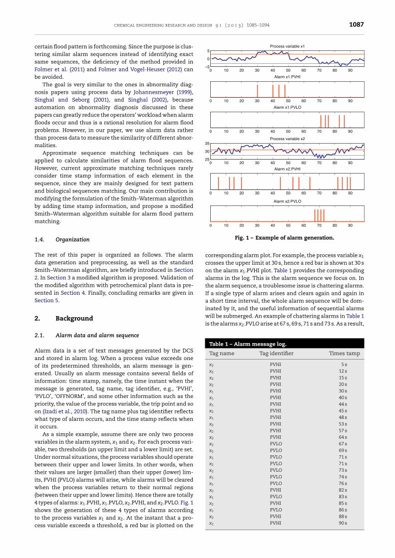

chemical engineering research and design 9 1 ( 2 0 1 3 ) 1085–1094 1087

ctsFb

nSapflptm

aHcsambSm

1

TdS2tsS

2

2

Aaoeim‘powi

vaUbtiw(4stc

0 10 20 30 40 50 60 70 80 90−5

0

5Process variable x1

0 10 20 30 40 50 60 70 80 90

Alarm x1.PVHI

0 10 20 30 40 50 60 70 80 90

Alarm x1.PVLO

0 10 20 30 40 50 60 70 80 9025

30

35Process variable x2

0 10 20 30 40 50 60 70 80 90

Alarm x2.PVHI

0 10 20 30 40 50 60 70 80 90

Alarm x2.PVLO

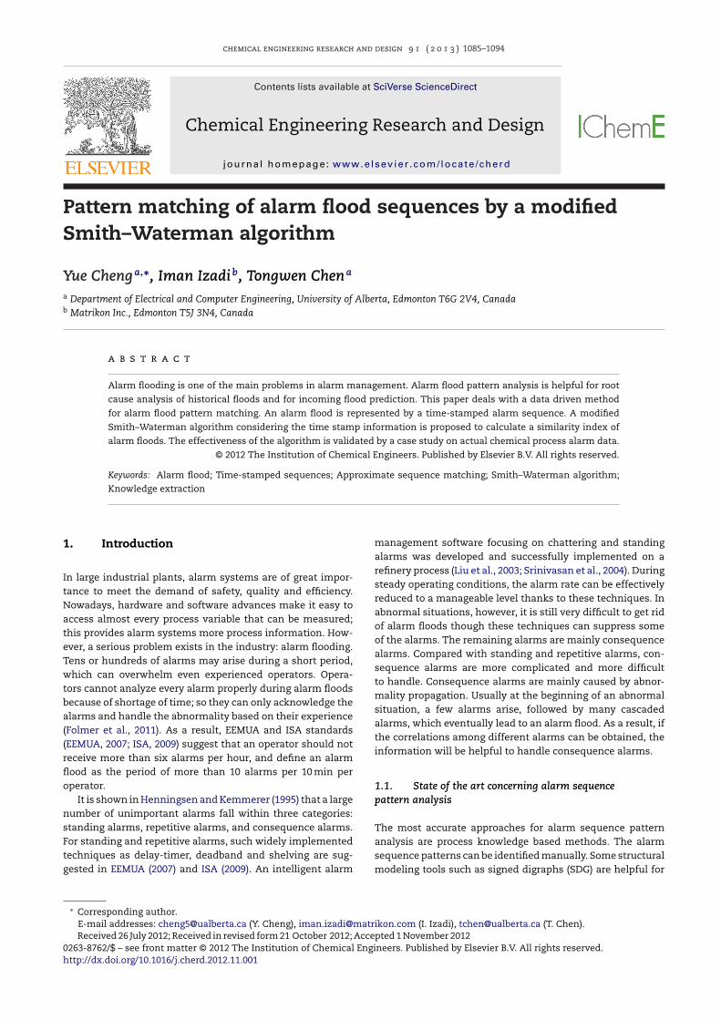
Fig. 1 – Example of alarm generation.

is the alarms x2.PVLO arise at 67 s, 69 s, 71 s and 73 s. As a result,

Table 1 – Alarm message log.

Tag name Tag identifier Times tamp

x2 PVHI 5 sx2 PVHI 12 sx2 PVHI 15 sx2 PVHI 20 sx1 PVHI 30 sx1 PVHI 40 sx1 PVHI 44 sx2 PVHI 45 sx1 PVHI 48 sx2 PVHI 53 sx2 PVHI 57 sx2 PVHI 64 sx2 PVLO 67 sx2 PVLO 69 sx1 PVLO 71 sx2 PVLO 71 sx2 PVLO 73 sx1 PVLO 74 sx1 PVLO 76 sx2 PVHI 82 sx1 PVLO 83 sx2 PVHI 85 sx1 PVLO 86 s

ertain flood pattern is forthcoming. Since the purpose is clus-ering similar alarm sequences instead of identifying exactame sequences, the deficiency of the method provided inolmer et al. (2011) and Folmer and Vogel-Heuser (2012) cane avoided.

The goal is very similar to the ones in abnormality diag-osis papers using process data by Johannesmeyer (1999),inghal and Seborg (2001), and Singhal (2002), becauseutomation on abnormality diagnosis discussed in theseapers can greatly reduce the operators’ workload when alarmoods occur and thus is a rational resolution for alarm floodroblems. However, in our paper, we use alarm data ratherhan process data to measure the similarity of different abnor-

alities.Approximate sequence matching techniques can be

pplied to calculate similarities of alarm flood sequences.owever, current approximate matching techniques rarelyonsider time stamp information of each element in theequence, since they are mainly designed for text patternnd biological sequences matching. Our main contribution isodifying the formulation of the Smith–Waterman algorithm

y adding time stamp information, and propose a modifiedmith–Waterman algorithm suitable for alarm flood patternatching.

.4. Organization

he rest of this paper is organized as follows. The alarmata generation and preprocessing, as well as the standardmith–Waterman algorithm, are briefly introduced in Section. In Section 3 a modified algorithm is proposed. Validation ofhe modified algorithm with petrochemical plant data is pre-ented in Section 4. Finally, concluding remarks are given inection 5.

. Background

.1. Alarm data and alarm sequence

larm data is a set of text messages generated by the DCSnd stored in alarm log. When a process value exceeds onef its predetermined thresholds, an alarm message is gen-rated. Usually an alarm message contains several fields ofnformation: time stamp, namely, the time instant when the

essage is generated, tag name, tag identifier, e.g., ‘PVHI’,PVLO’, ‘OFFNORM’, and some other information such as theriority, the value of the process variable, the trip point and son (Izadi et al., 2010). The tag name plus tag identifier reflectshat type of alarm occurs, and the time stamp reflects when

t occurs.As a simple example, assume there are only two process

ariables in the alarm system, x1 and x2. For each process vari-ble, two thresholds (an upper limit and a lower limit) are set.nder normal situations, the process variables should operateetween their upper and lower limits. In other words, whenheir values are larger (smaller) than their upper (lower) lim-ts, PVHI (PVLO) alarms will arise, while alarms will be cleared

hen the process variables return to their normal regionsbetween their upper and lower limits). Hence there are totally

types of alarms: x1.PVHI, x1.PVLO, x2.PVHI, and x2.PVLO. Fig. 1hows the generation of these 4 types of alarms according

o the process variables x1 and x2. At the instant that a pro-ess variable exceeds a threshold, a red bar is plotted on the

corresponding alarm plot. For example, the process variable x1

crosses the upper limit at 30 s, hence a red bar is shown at 30 son the alarm x1.PVHI plot. Table 1 provides the correspondingalarms in the log. This is the alarm sequence we focus on. Inthe alarm sequence, a troublesome issue is chattering alarms.If a single type of alarm arises and clears again and again ina short time interval, the whole alarm sequence will be dom-inated by it, and the useful information of sequential alarmswill be submerged. An example of chattering alarms in Table 1

x2 PVHI 88 sx2 PVHI 90 s

1088 chemical engineering research and design 9 1 ( 2 0 1 3 ) 1085–1094

the alarm sequence should be preprocessed to eliminate thechattering alarms before it is used for flood pattern analysis.A simple but effective way is to combine alarms of the sametype that occur within a short time.

2.2. Brief introduction of the Smith–Watermanalgorithm

The Smith–Waterman algorithm was first proposed in Smithand Waterman (1981). Its objective is “to find a pair of seg-ments, one from each of two long sequences, such that there isno other pair of segments with greater similarity (homology)”(Smith and Waterman, 1981).

The Smith–Waterman algorithm is a local sequence align-ment method. Before discussing the algorithm, we firstintroduce the concept of local alignment. Given a pair of sym-bolic segments, one from each of two symbolic sequences, wecan equalize the length of the two segments by inserting gaps(symbol ‘−’) in one or both of them (if the two segments havethe same length, we can also choose to insert no gap). Theneach symbol in one segment has a corresponding symbol inthe other segment at the same position. This is called align-ment. Since the two symbolic segments are two contiguoussubsequences of the two symbolic sequences, respectively, thealignment on the pair of segments is called local alignment ofthe two sequences.

For example, consider two symbolic segments:

X = [4 5 4 6 7]

Y = [6 6 7 4].

An alignment of this pair of segments is:

X′ = [4 5 4 6 7 −]

Y′ = [6 − − 6 7 4].

The two aligned segments have the same length 6. Each sym-bol in aligned segment X′ has a corresponding symbol in thealigned segment Y′, and the two symbols compose a sym-bolic pair. For instance, the first symbolic pair of the alignedsegments X′ and Y′ is (4, 6) and the second pair is (5, −).

Obviously, for one pair of segments there are a hugeamount of different alignments since gaps can be added arbi-trarily. Consider the example mentioned above, we can alsoalign the pair of symbolic segments as:

X′1 = [4 5 4 6 7 − −]

Y′1 = [6 − 6 − − 7 4],

or

X′2 = [4 5 4 6 7]

Y′2 = [6 − 6 7 4].

As a result, a scoring system is required to differentiate goodalignments from bad ones, and the similarity of the two sym-bolic segments should depend on the optimal alignment.

For a symbolic pair (a, b) in a pair of aligned symbolicsegments, where a and b are two symbols, e.g., two discreteevents, two letters, two nucleic acid bases, if neither a nor b isthe gap symbol ‘−’, a similarity score function s(a, b) : × →R, where is the alphabet of the concerned sequences, isprovided. The value of the similarity score function s(a, b) ispositive for a match (a = b), and is non-positive for a mismatch

(a /= b). Usually, a uniform score for all matched pairs (keptat 1) and a uniform negative score � for all mismatched pairs

are chosen if there is no additional prior information on thesymbols.

For a symbolic pair (a, b) including a gap symbol ‘−’, the sim-ilarity score is always negative as a penalty of inserting a gap.The value is related to l, the number of contiguous gap sym-bols prior to the current gap. In Smith and Waterman (1981),if l is 0, it is called opening a gap, which suffers a heavierpenalty. In the case that l > 0, it is called extending a gap, anda lighter penalty is used. In the case that opening a gap is notof greater significance, a uniform penalty value ı for all l ispreferred, since it can simplify the algorithm. Therefore, theuniform penalty value ı is used in our paper.

The similarity score of an alignment is the summation ofall the similarity scores of its symbolic pairs. The similarityscore calculation of the aligned segments X′ and Y′ is shownbelow.

Rewrite the alignment:

X′ = [4 5 4 6 7 −]

Y′ = [6 − − 6 7 4].

By using the uniform gap penalty value ı = −0.4 and similarityscore function

s(a, b) ={

1, if a = b

−0.6, if a /= b

we can calculate the similarity score of this alignment as:

s(4, 6) + ı + ı + s(6, 6) + s(7, 7) + ı

= −0.6 + (−0.4) + (−0.4) + 1 + 1 + (−0.4)

= 0.2.

The higher the similarity score is, the better the alignmentis. The alignment of a segment pair that have the highestsimilarity score is the optimal alignment of this pair, andthe corresponding similarity score is defined as the similarityindex of this segment pair.

Given concepts of alignment and the similarity index ofa segment pair, it is easy to formulate the local alignmentproblem.

Consider two symbolic sequences with arbitrary lengths:

A = [a1 a2 · · · aM]

B = [b1 b2 · · · bN],

where am, bn ∈ ˙, m = 1, 2, . . ., M, n = 1, 2, . . ., N. Ai:p and Bj:q

denote segments, or called contiguous subsequences, of A andB, respectively:

Ai:p = [ai ai+1 · · · ap]

Bj:q = [bj bj+1 · · · bq].

I(Ai:p, Bj:q) denotes the similarity index of the segment pair (Ai:p,Bj:q). The goal of the local alignment problem is searching forthe optimal segment pair whose similarity index is the high-est among all segment pairs. This highest similarity index isthen defined as the similarity index of the two sequences Aand B, which is denoted by S(A, B). The only exception is thatthe two sequences are totally different, and all the segmentpairs have a negative similarity index. In this case, S(A, B) isset to be 0, which means no similarity at all. In a nut shell,

the optimal local alignment of sequences A and B is the opti-mal alignment of the optimal segment pair of two sequences,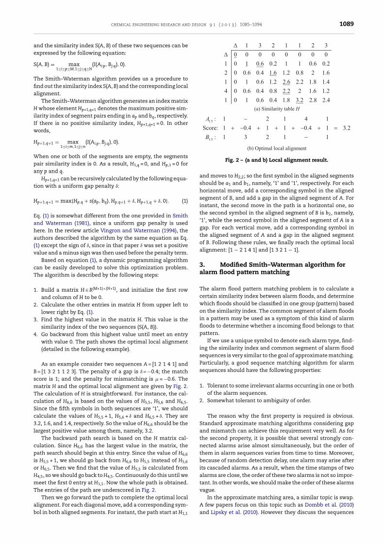

chemical engineering research and design 9 1 ( 2 0 1 3 ) 1085–1094 1089

ae

S

Tfia

HiIw

H

Wpa

t

H

Eaha(v

cT

1

2

3

4

BsmTcSc3l

cpioHmT

ab

nd the similarity index S(A, B) of these two sequences can bexpressed by the following equation:

(A, B) = max1≤i≤p≤M,1≤j≤q≤N

(I(Ai:p, Bj:q), 0).

he Smith–Waterman algorithm provides us a procedure tond out the similarity index S(A, B) and the corresponding locallignment.

The Smith–Waterman algorithm generates an index matrix whose element Hp+1,q+1 denotes the maximum positive sim-

larity index of segment pairs ending in ap and bq, respectively.f there is no positive similarity index, Hp+1,q+1 = 0. In otherords,

p+1,q+1 = max1≤i≤m,1≤j≤n

(I(Ai:p, Bj:q), 0).

hen one or both of the segments are empty, the segmentsair similarity index is 0. As a result, H1,q = 0, and Hp,1 = 0 forny p and q.

Hp+1,q+1 can be recursively calculated by the following equa-ion with a uniform gap penalty ı:

p+1,q+1 = max{Hp,q + s(ap, bq), Hp,q+1 + ı, Hp+1,q + ı, 0}. (1)

q. (1) is somewhat different from the one provided in Smithnd Waterman (1981), since a uniform gap penalty is usedere. In the review article Vingron and Waterman (1994), theuthors described the algorithm by the same equation as Eq.1) except the sign of ı, since in that paper ı was set a positivealue and a minus sign was then used before the penalty term.

Based on equation (1), a dynamic programming algorithman be easily developed to solve this optimization problem.he algorithm is described by the following steps:

. Build a matrix H ∈ R(M+1)×(N+1), and initialize the first rowand column of H to be 0.

. Calculate the other entries in matrix H from upper left tolower right by Eq. (1).

. Find the highest value in the matrix H. This value is thesimilarity index of the two sequences (S(A, B)).

. Go backward from this highest value until meet an entrywith value 0. The path shows the optimal local alignment(detailed in the following example).

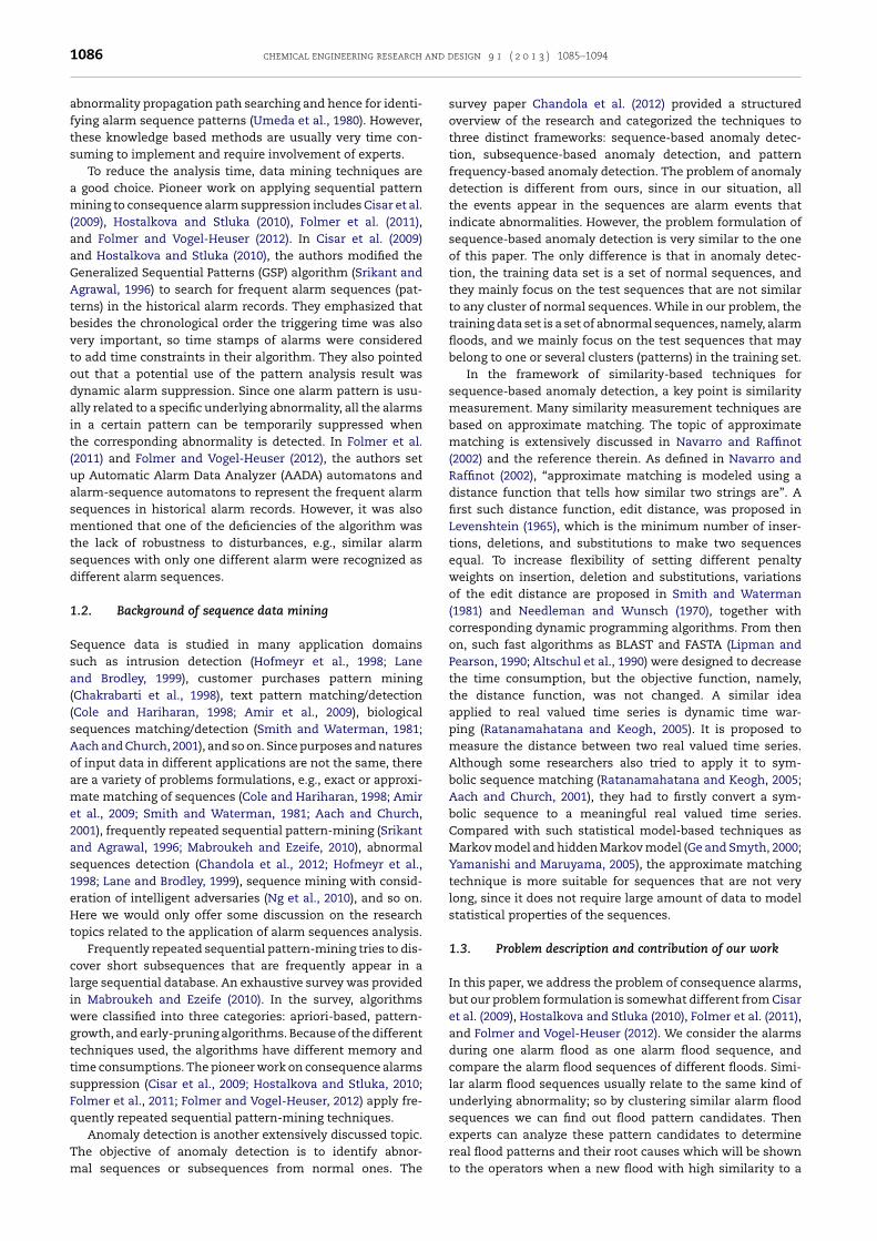
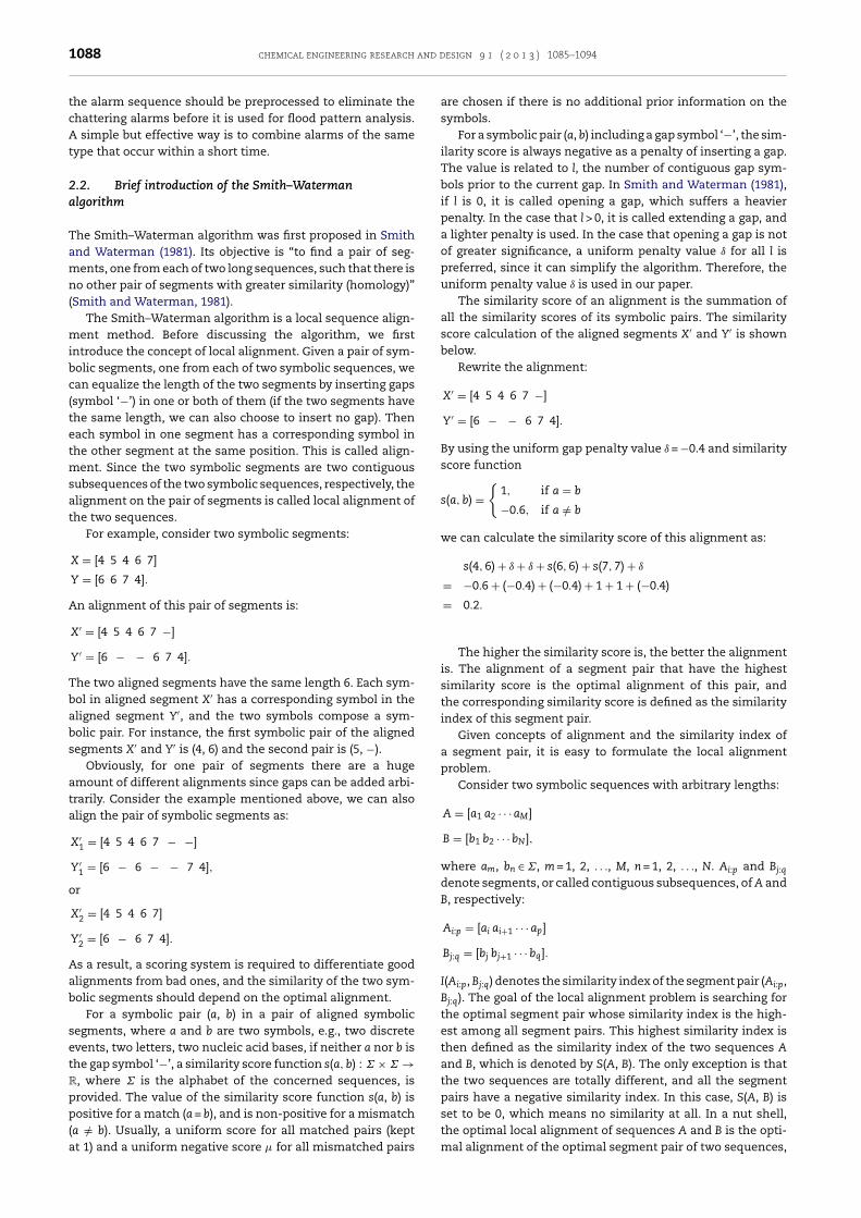
As an example consider two sequences A = [1 2 1 4 1] and = [1 3 2 1 1 2 3]. The penalty of a gap is ı = −0.4; the matchcore is 1; and the penalty for mismatching is � = −0.6. Theatrix H and the optimal local alignment are given by Fig. 2.

he calculation of H is straightforward. For instance, the cal-ulation of H6,6 is based on the values of H5,5, H5,6 and H6,5.ince the fifth symbols in both sequences are ‘1’, we shouldalculate the values of H5,5 + 1, H5,6 + ı and H6,5 + ı. They are.2, 1.6, and 1.4, respectively. So the value of H6,6 should be theargest positive value among them, namely, 3.2.

The backward path search is based on the H matrix cal-ulation. Since H6,6 has the largest value in the matrix, theath search should begin at this entry. Since the value of H6,6

s H5,5 + 1, we should go back from H6,6 to H5,5 instead of H5,6

r H6,5. Then we find that the value of H5,5 is calculated from

4,5, so we should go back to H4,5. Continuously do this until weeet the first 0 entry at H1,1. Now the whole path is obtained.

he entries of the path are underscored in Fig. 2.Then we go forward the path to complete the optimal local

lignment. For each diagonal move, add a corresponding sym-ol in both aligned segments. For instant, the path start at H1,1

Fig. 2 – (a and b) Local alignment result.

and moves to H2,2; so the first symbol in the aligned segmentsshould be a1 and b1, namely, ‘1’ and ‘1’, respectively. For eachhorizontal move, add a corresponding symbol in the alignedsegment of B, and add a gap in the aligned segment of A. Forinstant, the second move in the path is a horizontal one, sothe second symbol in the aligned segment of B is b2, namely,‘1’, while the second symbol in the aligned segment of A is agap. For each vertical move, add a corresponding symbol inthe aligned segment of A and a gap in the aligned segmentof B. Following these rules, we finally reach the optimal localalignment: [1 − 2 1 4 1] and [1 3 2 1 − 1].

3. Modified Smith–Waterman algorithm foralarm flood pattern matching

The alarm flood pattern matching problem is to calculate acertain similarity index between alarm floods, and determinewhich floods should be classified in one group (pattern) basedon the similarity index. The common segment of alarm floodsin a pattern may be used as a symptom of this kind of alarmfloods to determine whether a incoming flood belongs to thatpattern.

If we use a unique symbol to denote each alarm type, find-ing the similarity index and common segment of alarm floodsequences is very similar to the goal of approximate matching.Particularly, a good sequence matching algorithm for alarmsequences should have the following properties:

1. Tolerant to some irrelevant alarms occurring in one or bothof the alarm sequences.

2. Somewhat tolerant to ambiguity of order.

The reason why the first property is required is obvious.Standard approximate matching algorithms considering gapand mismatch can achieve this requirement very well. As forthe second property, it is possible that several strongly con-nected alarms arise almost simultaneously, but the order ofthem in alarm sequences varies from time to time. Moreover,because of random detection delay, one alarm may arise afterits cascaded alarms. As a result, when the time stamps of twoalarms are close, the order of these two alarms is not so impor-tant. In other words, we should make the order of these alarmsvague.

In the approximate matching area, a similar topic is swap.

A few papers focus on this topic such as Dombb et al. (2010)and Lipsky et al. (2010). However they discuss the sequences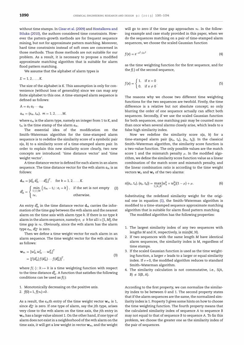

1090 chemical engineering research and design 9 1 ( 2 0 1 3 ) 1085–1094

without time stamps. In Cisar et al. (2009) and Hostalkova andStluka (2010), the authors considered time constraints. How-ever the pattern-growth methods are for frequent sequencemining, but not for approximate pattern matching. Moreover,hard time constraints instead of soft ones are concerned inthose methods. Thus those methods are not suitable for ourproblem. As a result, it is necessary to propose a modifiedapproximate matching algorithm that is suitable for alarmflood pattern matching.

We assume that the alphabet of alarm types is

= 1, 2, . . . , K.

The size of the alphabet is K. This assumption is only for con-venience (without loss of generality) since we can map anyfinite alphabet to this one. A time-stamped alarm sequence isdefined as follows:

A = a1 a2 · · · aM

am = (em, tm), m = 1, 2, . . . , M,

where em is the alarm type, namely an integer from 1 to K, andtm is the time stamp of the alarm am.

The essential idea of the modification on theSmith–Waterman algorithm for the time-stamped alarmsequence is to redefine the similarity score of a symbolic pairs(a, b) to a similarity score of a time-stamped alarm pair. Inorder to explain this new similarity score clearly, two newconcepts are introduced: ‘time distance vector’ and ‘timeweight vector’.

A time distance vector is defined for each alarm in an alarmsequence. The time distance vector for the mth alarm am is asfollows:

dm = [d1m d2

m · · · dKm]T, for k = 1, 2, . . . , K.

dkm =

{min

1≤i≤M

{|tm − ti| : ei = k

}, if the set is not empty

∞, otherwise,

(2)

An entry dkm in the time distance vector dm carries the infor-

mation of the time gap between the mth alarm and the nearestalarm on the time axis with alarm type k. If there is no type kalarm in the alarm sequence, namely ei /= k for all i ∈ [1, M], thetime gap is ∞. Obviously, since the mth alarm has the alarmtype em, dem

m is zero.Then we define a time weight vector for each alarm in an

alarm sequence. The time weight vector for the mth alarm isas follows:

wm = [w1m w2

m · · · wKm]T

= [f (d1m) f (d2

m) · · · f (dKm)]T,

(3)

where f ( · ) : R �→ R is a time weighting function with respectto the time distance dk

m. A function that satisfies the followingconditions can be used as f(·):

1. Monotonically decreasing on the positive axis.2. f(0) = 1, f(∞) =0 .

As a result, the emth entry of the time weight vector wm is 1,since dem

m is zero. If one type of alarm, say the jth type, arisesvery close to the mth alarm on the time axis, the jth entry inwm has a large value almost 1. On the other hand, if one type of

alarm does not exist in a neighborhood of the mth alarm on thetime axis, it will get a low weight in vector wm, and the weight

will go to zero if the time gap approaches ∞. In the follow-ing example and case study provided in this paper, when wedo the sequences matching on a pair of time-stamped alarmsequences, we choose the scaled Gaussian function

f (x) = e−x2/2�2(4)

as the time weighting function for the first sequence, and forthe f(·) of the second sequence,

f (x) ={

1, if x = 0

0, if x /= 0. (5)

The reasons why we choose two different time weightingfunctions for the two sequences are twofold. Firstly, the timedifference is a relative but not absolute concept; so onlyblurring the order of one sequence actually can affect bothsequences. Secondly, if we use the scaled Gaussian functionfor both sequences, one matching pair may be counted morethan once when several alarms closely arise, which leads to afalse high similarity index.

Now we redefine the similarity score s(a, b) for atime-stamped alarm pair ((ea, ta), (eb, tb)). In the classicalSmith–Waterman algorithm, the similarity score function isa two-value function. The only possible values are the matchscore 1 and the mismatch penalty �. In the modified algo-rithm, we define the similarity score function value as a linearcombination of the match score and mismatch penalty, andthe linear combination ratio is according to the time weightvectors wa and wb of the two alarms:

s((ea, ta), (eb, tb)) = max1≤k≤K

[wka × wk

b](1 − �) + �. (6)

Substituting the redefined similarity weight for the origi-nal one in equation (1), the Smith–Waterman algorithm ismodified to a time-stamped sequence approximate matchingalgorithm that is suitable for alarm flood pattern matching.

The modified algorithm has the following properties:

1. The largest similarity index of any two sequences withlengths M and N, respectively, is min(M, N).

2. If two sequences with the same length M have identicalalarm sequences, the similarity index is M, regardless oftime stamps.

3. If the scaled Gaussian function is used as the time weight-ing function, a larger � leads to a larger or equal similarityindex. If � = 0, the modified algorithm reduces to standardSmith–Waterman algorithm.

4. The similarity calculation is not commutative, i.e., S(A,B) /= S(B, A).

According to the first property, we can normalize the similar-ity index to be between 0 and 1. The second property statesthat if the alarm sequences are the same, the normalized sim-ilarity index is 1. Property 3 gives some hints on how to choosethe time weighting function. The fourth property means thatthe calculated similarity index of sequence A to sequence Bmay not equal to that of sequence B to sequence A. To fix this

problem, we choose the greater one as the similarity index ofthe pair of sequences.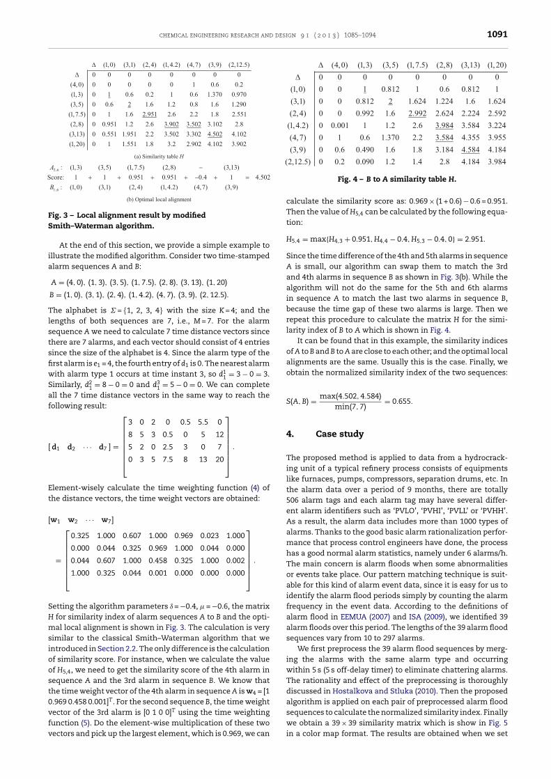

chemical engineering research and design 9 1 ( 2 0 1 3 ) 1085–1094 1091

Fig. 3 – Local alignment result by modifiedS

ia

TlstsfiwSaf

[

Et

[

SHmsioost0vfv

mith–Waterman algorithm.

At the end of this section, we provide a simple example tollustrate the modified algorithm. Consider two time-stampedlarm sequences A and B:

A = (4, 0), (1, 3), (3, 5), (1, 7.5), (2, 8), (3, 13), (1, 20)

B = (1, 0), (3, 1), (2, 4), (1, 4.2), (4, 7), (3, 9), (2, 12.5).

he alphabet is = {1, 2, 3, 4} with the size K = 4; and theengths of both sequences are 7, i.e., M = 7. For the alarmequence A we need to calculate 7 time distance vectors sincehere are 7 alarms, and each vector should consist of 4 entriesince the size of the alphabet is 4. Since the alarm type of therst alarm is e1 = 4, the fourth entry of d1 is 0. The nearest alarmith alarm type 1 occurs at time instant 3, so d1

1 = 3 − 0 = 3.imilarly, d2

1 = 8 − 0 = 0 and d31 = 5 − 0 = 0. We can complete

ll the 7 time distance vectors in the same way to reach theollowing result:

d1 d2 · · · d7 ] =

⎡⎢⎢⎢⎢⎢⎣

3 0 2 0 0.5 5.5 0

8 5 3 0.5 0 5 12

5 2 0 2.5 3 0 7

0 3 5 7.5 8 13 20

⎤⎥⎥⎥⎥⎥⎦ .

lement-wisely calculate the time weighting function (4) ofhe distance vectors, the time weight vectors are obtained:

w1 w2 · · · w7]

=

⎡⎢⎢⎢⎢⎢⎣

0.325 1.000 0.607 1.000 0.969 0.023 1.000

0.000 0.044 0.325 0.969 1.000 0.044 0.000

0.044 0.607 1.000 0.458 0.325 1.000 0.002

1.000 0.325 0.044 0.001 0.000 0.000 0.000

⎤⎥⎥⎥⎥⎥⎦ .

etting the algorithm parameters ı = −0.4, � = −0.6, the matrix for similarity index of alarm sequences A to B and the opti-al local alignment is shown in Fig. 3. The calculation is very

imilar to the classical Smith–Waterman algorithm that wentroduced in Section 2.2. The only difference is the calculationf similarity score. For instance, when we calculate the valuef H5,4, we need to get the similarity score of the 4th alarm inequence A and the 3rd alarm in sequence B. We know thathe time weight vector of the 4th alarm in sequence A is w4 = [1.969 0.458 0.001]T. For the second sequence B, the time weightector of the 3rd alarm is [0 1 0 0]T using the time weighting

unction (5). Do the element-wise multiplication of these twoectors and pick up the largest element, which is 0.969, we can

Fig. 4 – B to A similarity table H.

calculate the similarity score as: 0.969 × (1 + 0.6) − 0.6 = 0.951.Then the value of H5,4 can be calculated by the following equa-tion:

H5,4 = max{H4,3 + 0.951, H4,4 − 0.4, H5,3 − 0.4, 0} = 2.951.

Since the time difference of the 4th and 5th alarms in sequenceA is small, our algorithm can swap them to match the 3rdand 4th alarms in sequence B as shown in Fig. 3(b). While thealgorithm will not do the same for the 5th and 6th alarmsin sequence A to match the last two alarms in sequence B,because the time gap of these two alarms is large. Then werepeat this procedure to calculate the matrix H for the simi-larity index of B to A which is shown in Fig. 4.

It can be found that in this example, the similarity indicesof A to B and B to A are close to each other; and the optimal localalignments are the same. Usually this is the case. Finally, weobtain the normalized similarity index of the two sequences:

S(A, B) = max(4.502, 4.584)min(7, 7)

= 0.655.

4. Case study

The proposed method is applied to data from a hydrocrack-ing unit of a typical refinery process consists of equipmentslike furnaces, pumps, compressors, separation drums, etc. Inthe alarm data over a period of 9 months, there are totally506 alarm tags and each alarm tag may have several differ-ent alarm identifiers such as ‘PVLO’, ‘PVHI’, ‘PVLL’ or ‘PVHH’.As a result, the alarm data includes more than 1000 types ofalarms. Thanks to the good basic alarm rationalization perfor-mance that process control engineers have done, the processhas a good normal alarm statistics, namely under 6 alarms/h.The main concern is alarm floods when some abnormalitiesor events take place. Our pattern matching technique is suit-able for this kind of alarm event data, since it is easy for us toidentify the alarm flood periods simply by counting the alarmfrequency in the event data. According to the definitions ofalarm flood in EEMUA (2007) and ISA (2009), we identified 39alarm floods over this period. The lengths of the 39 alarm floodsequences vary from 10 to 297 alarms.

We first preprocess the 39 alarm flood sequences by merg-ing the alarms with the same alarm type and occurringwithin 5 s (5 s off-delay timer) to eliminate chattering alarms.The rationality and effect of the preprocessing is thoroughlydiscussed in Hostalkova and Stluka (2010). Then the proposedalgorithm is applied on each pair of preprocessed alarm floodsequences to calculate the normalized similarity index. Finally

we obtain a 39 × 39 similarity matrix which is show in Fig. 5in a color map format. The results are obtained when we set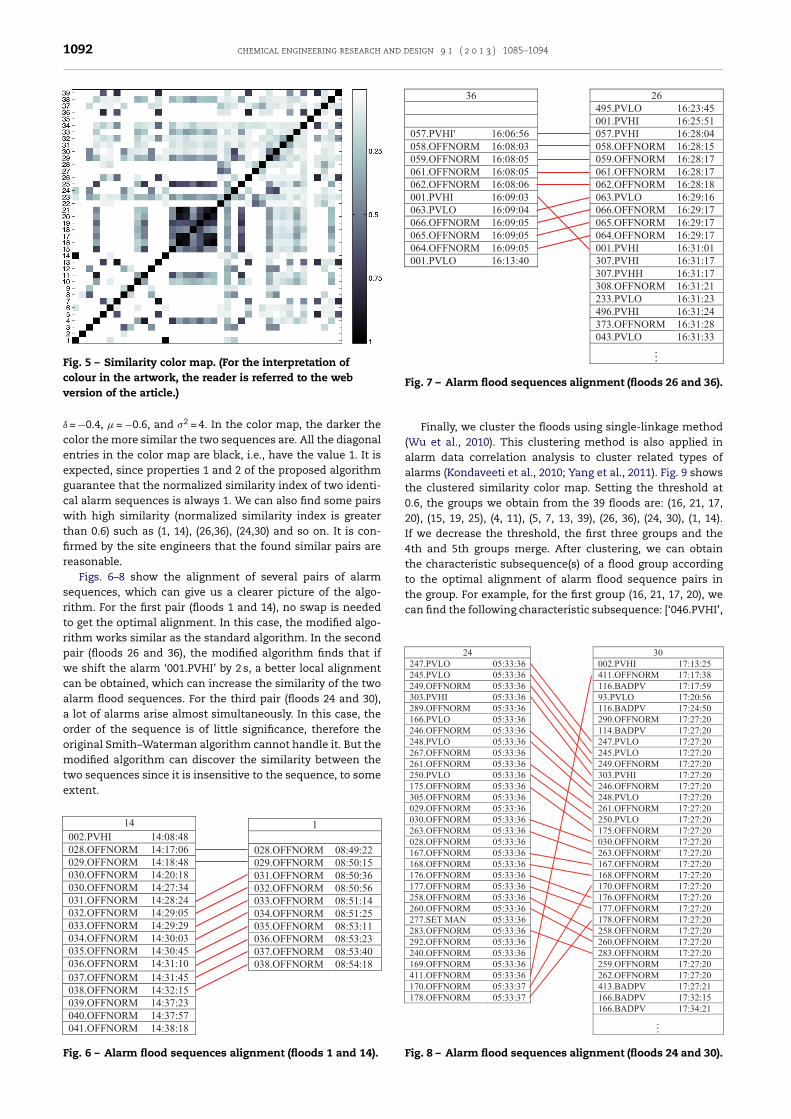

1092 chemical engineering research and design 9 1 ( 2 0 1 3 ) 1085–1094

Fig. 5 – Similarity color map. (For the interpretation ofcolour in the artwork, the reader is referred to the web Fig. 7 – Alarm flood sequences alignment (floods 26 and 36).

can find the following characteristic subsequence: [‘046.PVHI’,

version of the article.)

ı = −0.4, � = −0.6, and �2 = 4. In the color map, the darker thecolor the more similar the two sequences are. All the diagonalentries in the color map are black, i.e., have the value 1. It isexpected, since properties 1 and 2 of the proposed algorithmguarantee that the normalized similarity index of two identi-cal alarm sequences is always 1. We can also find some pairswith high similarity (normalized similarity index is greaterthan 0.6) such as (1, 14), (26,36), (24,30) and so on. It is con-firmed by the site engineers that the found similar pairs arereasonable.

Figs. 6–8 show the alignment of several pairs of alarmsequences, which can give us a clearer picture of the algo-rithm. For the first pair (floods 1 and 14), no swap is neededto get the optimal alignment. In this case, the modified algo-rithm works similar as the standard algorithm. In the secondpair (floods 26 and 36), the modified algorithm finds that ifwe shift the alarm ‘001.PVHI’ by 2 s, a better local alignmentcan be obtained, which can increase the similarity of the twoalarm flood sequences. For the third pair (floods 24 and 30),a lot of alarms arise almost simultaneously. In this case, theorder of the sequence is of little significance, therefore theoriginal Smith–Waterman algorithm cannot handle it. But themodified algorithm can discover the similarity between the

two sequences since it is insensitive to the sequence, to someextent.

Fig. 6 – Alarm flood sequences alignment (floods 1 and 14).

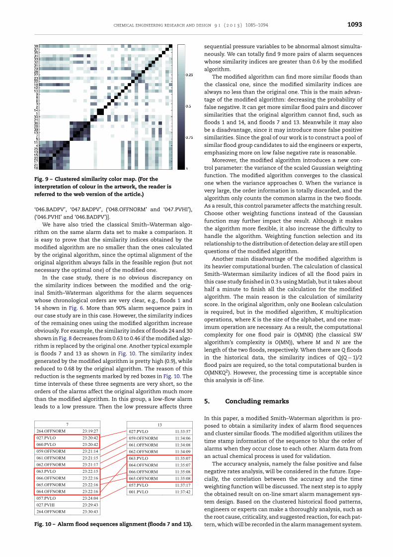
Finally, we cluster the floods using single-linkage method(Wu et al., 2010). This clustering method is also applied inalarm data correlation analysis to cluster related types ofalarms (Kondaveeti et al., 2010; Yang et al., 2011). Fig. 9 showsthe clustered similarity color map. Setting the threshold at0.6, the groups we obtain from the 39 floods are: (16, 21, 17,20), (15, 19, 25), (4, 11), (5, 7, 13, 39), (26, 36), (24, 30), (1, 14).If we decrease the threshold, the first three groups and the4th and 5th groups merge. After clustering, we can obtainthe characteristic subsequence(s) of a flood group accordingto the optimal alignment of alarm flood sequence pairs inthe group. For example, for the first group (16, 21, 17, 20), we

Fig. 8 – Alarm flood sequences alignment (floods 24 and 30).

chemical engineering research and design 9 1 ( 2 0 1 3 ) 1085–1094 1093

Fig. 9 – Clustered similarity color map. (For theinterpretation of colour in the artwork, the reader isr

‘(

rimbon

tiw1ooosrigrrtotl

F

eferred to the web version of the article.)

046.BADPV’, ‘047.BADPV’, (‘048.OFFNORM’ and ‘047.PVHI’),‘046.PVHI’ and ‘046.BADPV’)].

We have also tried the classical Smith–Waterman algo-ithm on the same alarm data set to make a comparison. Its easy to prove that the similarity indices obtained by the

odified algorithm are no smaller than the ones calculatedy the original algorithm, since the optimal alignment of theriginal algorithm always falls in the feasible region (but notecessary the optimal one) of the modified one.

In the case study, there is no obvious discrepancy onhe similarity indices between the modified and the orig-nal Smith–Waterman algorithms for the alarm sequences

hose chronological orders are very clear, e.g., floods 1 and4 shown in Fig. 6. More than 90% alarm sequence pairs inur case study are in this case. However, the similarity indicesf the remaining ones using the modified algorithm increasebviously. For example, the similarity index of floods 24 and 30hown in Fig. 8 decreases from 0.63 to 0.46 if the modified algo-ithm is replaced by the original one. Another typical examples floods 7 and 13 as shown in Fig. 10. The similarity indexenerated by the modified algorithm is pretty high (0.9), whileeduced to 0.68 by the original algorithm. The reason of thiseduction is the segments marked by red boxes in Fig. 10. Theime intervals of these three segments are very short, so therders of the alarms affect the original algorithm much more

han the modified algorithm. In this group, a low-flow alarmeads to a low pressure. Then the low pressure affects three

7264.OFFNORM 23:19:27 027.PVLO 23:20:42 060.PVLO 23:20:42 059.OFFNORM 23:21:14 061.OFFNORM 23:21:15 062.OFFNORM 23:21:17 063.PVLO 23:22:15 066.OFFNORM 23:22:16 065.OFFNORM 23:22:16 064.OFFNORM 23:22:16 057.PVLO 23:24:04 027.PVHI 23:29:43 264.OFFNORM 23:30:43

13027.PVLO 11:33:57 059.OFFNORM 11:34:06 061.OFFNORM 11:34:08 062.OFFNORM 11:34:09 063.PVLO 11:35:07 064.OFFNORM 11:35:07 066.OFFNORM 11:35:08 065.OFFNORM 11:35:08 057.PVLO 11:37:17 001.PVLO 11:37:42

ig. 10 – Alarm flood sequences alignment (floods 7 and 13).

sequential pressure variables to be abnormal almost simulta-neously. We can totally find 9 more pairs of alarm sequenceswhose similarity indices are greater than 0.6 by the modifiedalgorithm.

The modified algorithm can find more similar floods thanthe classical one, since the modified similarity indices arealways no less than the original one. This is the main advan-tage of the modified algorithm: decreasing the probability offalse negative. It can get more similar flood pairs and discoversimilarities that the original algorithm cannot find, such asfloods 1 and 14, and floods 7 and 13. Meanwhile it may alsobe a disadvantage, since it may introduce more false positivesimilarities. Since the goal of our work is to construct a pool ofsimilar flood group candidates to aid the engineers or experts,emphasizing more on low false negative rate is reasonable.

Moreover, the modified algorithm introduces a new con-trol parameter: the variance of the scaled Gaussian weightingfunction. The modified algorithm converges to the classicalone when the variance approaches 0. When the variance isvery large, the order information is totally discarded, and thealgorithm only counts the common alarms in the two floods.As a result, this control parameter affects the matching result.Choose other weighting functions instead of the Gaussianfunction may further impact the result. Although it makesthe algorithm more flexible, it also increase the difficulty tohandle the algorithm. Weighting function selection and itsrelationship to the distribution of detection delay are still openquestions of the modified algorithm.

Another main disadvantage of the modified algorithm isits heavier computational burden. The calculation of classicalSmith–Waterman similarity indices of all the flood pairs inthis case study finished in 0.3 s using Matlab, but it takes abouthalf a minute to finish all the calculation for the modifiedalgorithm. The main reason is the calculation of similarityscore. In the original algorithm, only one Boolean calculationis required, but in the modified algorithm, K multiplicationoperations, where K is the size of the alphabet, and one max-imum operation are necessary. As a result, the computationalcomplexity for one flood pair is O(MNK) (the classical SWalgorithm’s complexity is O(MN)), where M and N are thelength of the two floods, respectively. When there are Q floodsin the historical data, the similarity indices of Q(Q − 1)/2flood pairs are required, so the total computational burden isO(MNKQ2). However, the processing time is acceptable sincethis analysis is off-line.

5. Concluding remarks

In this paper, a modified Smith–Waterman algorithm is pro-posed to obtain a similarity index of alarm flood sequencesand cluster similar floods. The modified algorithm utilizes thetime stamp information of the sequence to blur the order ofalarms when they occur close to each other. Alarm data froman actual chemical process is used for validation.

The accuracy analysis, namely the false positive and falsenegative rates analysis, will be considered in the future. Espe-cially, the correlation between the accuracy and the timeweighting function will be discussed. The next step is to applythe obtained result on on-line smart alarm management sys-tem design. Based on the clustered historical flood patterns,engineers or experts can make a thoroughly analysis, such as

the root cause, criticality, and suggested reaction, for each pat-tern, which will be recorded in the alarm management system.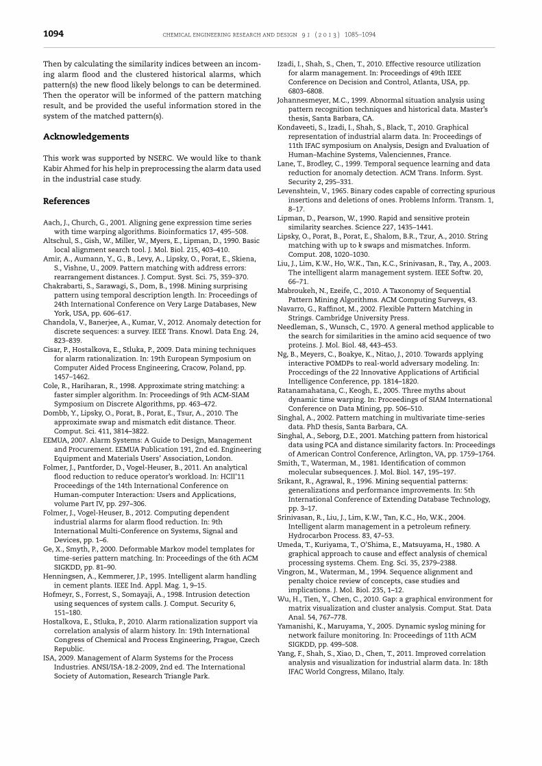

1094 chemical engineering research and design 9 1 ( 2 0 1 3 ) 1085–1094

Then by calculating the similarity indices between an incom-ing alarm flood and the clustered historical alarms, whichpattern(s) the new flood likely belongs to can be determined.Then the operator will be informed of the pattern matchingresult, and be provided the useful information stored in thesystem of the matched pattern(s).

Acknowledgements

This work was supported by NSERC. We would like to thankKabir Ahmed for his help in preprocessing the alarm data usedin the industrial case study.

References

Aach, J., Church, G., 2001. Aligning gene expression time serieswith time warping algorithms. Bioinformatics 17, 495–508.

Altschul, S., Gish, W., Miller, W., Myers, E., Lipman, D., 1990. Basiclocal alignment search tool. J. Mol. Biol. 215, 403–410.

Amir, A., Aumann, Y., G., B., Levy, A., Lipsky, O., Porat, E., Skiena,S., Vishne, U., 2009. Pattern matching with address errors:rearrangement distances. J. Comput. Syst. Sci. 75, 359–370.

Chakrabarti, S., Sarawagi, S., Dom, B., 1998. Mining surprisingpattern using temporal description length. In: Proceedings of24th International Conference on Very Large Databases, NewYork, USA, pp. 606–617.

Chandola, V., Banerjee, A., Kumar, V., 2012. Anomaly detection fordiscrete sequences: a survey. IEEE Trans. Knowl. Data Eng. 24,823–839.

Cisar, P., Hostalkova, E., Stluka, P., 2009. Data mining techniquesfor alarm rationalization. In: 19th European Symposium onComputer Aided Process Engineering, Cracow, Poland, pp.1457–1462.

Cole, R., Hariharan, R., 1998. Approximate string matching: afaster simpler algorithm. In: Proceedings of 9th ACM-SIAMSymposium on Discrete Algorithms, pp. 463–472.

Dombb, Y., Lipsky, O., Porat, B., Porat, E., Tsur, A., 2010. Theapproximate swap and mismatch edit distance. Theor.Comput. Sci. 411, 3814–3822.

EEMUA, 2007. Alarm Systems: A Guide to Design, Managementand Procurement. EEMUA Publication 191, 2nd ed. EngineeringEquipment and Materials Users’ Association, London.

Folmer, J., Pantforder, D., Vogel-Heuser, B., 2011. An analyticalflood reduction to reduce operator’s workload. In: HCII’11Proceedings of the 14th International Conference onHuman-computer Interaction: Users and Applications,volume Part IV, pp. 297–306.

Folmer, J., Vogel-Heuser, B., 2012. Computing dependentindustrial alarms for alarm flood reduction. In: 9thInternational Multi-Conference on Systems, Signal andDevices, pp. 1–6.

Ge, X., Smyth, P., 2000. Deformable Markov model templates fortime-series pattern matching. In: Proceedings of the 6th ACMSIGKDD, pp. 81–90.

Henningsen, A., Kemmerer, J.P., 1995. Intelligent alarm handlingin cement plants. IEEE Ind. Appl. Mag. 1, 9–15.

Hofmeyr, S., Forrest, S., Somayaji, A., 1998. Intrusion detectionusing sequences of system calls. J. Comput. Security 6,151–180.

Hostalkova, E., Stluka, P., 2010. Alarm rationalization support viacorrelation analysis of alarm history. In: 19th InternationalCongress of Chemical and Process Engineering, Prague, CzechRepublic.

ISA, 2009. Management of Alarm Systems for the Process

Industries. ANSI/ISA-18.2-2009, 2nd ed. The InternationalSociety of Automation, Research Triangle Park.

Izadi, I., Shah, S., Chen, T., 2010. Effective resource utilizationfor alarm management. In: Proceedings of 49th IEEEConference on Decision and Control, Atlanta, USA, pp.6803–6808.

Johannesmeyer, M.C., 1999. Abnormal situation analysis usingpattern recognition techniques and historical data. Master’sthesis, Santa Barbara, CA.

Kondaveeti, S., Izadi, I., Shah, S., Black, T., 2010. Graphicalrepresentation of industrial alarm data. In: Proceedings of11th IFAC symposium on Analysis, Design and Evaluation ofHuman–Machine Systems, Valenciennes, France.

Lane, T., Brodley, C., 1999. Temporal sequence learning and datareduction for anomaly detection. ACM Trans. Inform. Syst.Security 2, 295–331.

Levenshtein, V., 1965. Binary codes capable of correcting spuriousinsertions and deletions of ones. Problems Inform. Transm. 1,8–17.

Lipman, D., Pearson, W., 1990. Rapid and sensitive proteinsimilarity searches. Science 227, 1435–1441.

Lipsky, O., Porat, B., Porat, E., Shalom, B.R., Tzur, A., 2010. Stringmatching with up to k swaps and mismatches. Inform.Comput. 208, 1020–1030.

Liu, J., Lim, K.W., Ho, W.K., Tan, K.C., Srinivasan, R., Tay, A., 2003.The intelligent alarm management system. IEEE Softw. 20,66–71.

Mabroukeh, N., Ezeife, C., 2010. A Taxonomy of SequentialPattern Mining Algorithms. ACM Computing Surveys, 43.

Navarro, G., Raffinot, M., 2002. Flexible Pattern Matching inStrings. Cambridge University Press.

Needleman, S., Wunsch, C., 1970. A general method applicable tothe search for similarities in the amino acid sequence of twoproteins. J. Mol. Biol. 48, 443–453.

Ng, B., Meyers, C., Boakye, K., Nitao, J., 2010. Towards applyinginteractive POMDPs to real-world adversary modeling. In:Proccedings of the 22 Innovative Applications of ArtificialIntelligence Conference, pp. 1814–1820.

Ratanamahatana, C., Keogh, E., 2005. Three myths aboutdynamic time warping. In: Proceedings of SIAM InternationalConference on Data Mining, pp. 506–510.

Singhal, A., 2002. Pattern matching in multivariate time-seriesdata. PhD thesis, Santa Barbara, CA.

Singhal, A., Seborg, D.E., 2001. Matching pattern from historicaldata using PCA and distance similarity factors. In: Proceedingsof American Control Conference, Arlington, VA, pp. 1759–1764.

Smith, T., Waterman, M., 1981. Identification of commonmolecular subsequences. J. Mol. Biol. 147, 195–197.

Srikant, R., Agrawal, R., 1996. Mining sequential patterns:generalizations and performance improvements. In: 5thInternational Conference of Extending Database Technology,pp. 3–17.

Srinivasan, R., Liu, J., Lim, K.W., Tan, K.C., Ho, W.K., 2004.Intelligent alarm management in a petroleum refinery.Hydrocarbon Process. 83, 47–53.

Umeda, T., Kuriyama, T., O’Shima, E., Matsuyama, H., 1980. Agraphical approach to cause and effect analysis of chemicalprocessing systems. Chem. Eng. Sci. 35, 2379–2388.

Vingron, M., Waterman, M., 1994. Sequence alignment andpenalty choice review of concepts, case studies andimplications. J. Mol. Biol. 235, 1–12.

Wu, H., Tien, Y., Chen, C., 2010. Gap: a graphical environment formatrix visualization and cluster analysis. Comput. Stat. DataAnal. 54, 767–778.

Yamanishi, K., Maruyama, Y., 2005. Dynamic syslog mining fornetwork failure monitoring. In: Proceedings of 11th ACMSIGKDD, pp. 499–508.

Yang, F., Shah, S., Xiao, D., Chen, T., 2011. Improved correlation

analysis and visualization for industrial alarm data. In: 18thIFAC World Congress, Milano, Italy.