Embed Size (px)
Citation preview
Applied Mathematics and Computation 205 (2008) 778–791
Contents lists available at ScienceDirect
Applied Mathematics and Computation
journal homepage: www.elsevier .com/ locate /amc
Comparison of classical control and intelligent control for a MIMO system
Jih-Gau Juang *, Ren-Wei Lin, Wen-Kai LiuDepartment of Communications and Guidance Engineering, National Taiwan Ocean University, Keelung, Taiwan
a r t i c l e i n f o
Keywords:Classical controlIntelligent control
Fuzzy systemGenetic algorithmMIMO system0096-3003/$ - see front matter � 2008 Elsevier Incdoi:10.1016/j.amc.2008.05.061
* Corresponding author.E-mail address: [email protected] (J.-G.
a b s t r a c t
This paper presents several classical control schemes and intelligent control schemes of anexperimental propeller setup, which is called the twin rotor multi-input multi-output(MIMO) system. The objective of this study is to decouple the twin rotor MIMO system intothe horizontal plane and vertical plane, and perform setpoint control that makes the beamof the twin rotor MIMO system move quickly and accurately in order to track a trajectoryor to reach specified positions. We utilize the conventional control and intelligent controltechniques in the vertical and horizontal planes of the twin rotor MIMO system. In classicalcontrol, three of the most popular controller design techniques are utilized in this study.These are the Ziegler–Nichols Proportional–Integral–Derivative (PID) rule, the gain marginand phase margin rule, and the pole placement method. Intelligent control is also proposedin this paper in order to improve the attitude tracking accuracy of the twin rotor MIMOsystem. Intelligent control designs are based on fuzzy logic system and genetic algorithm.Simulations show that the intelligent controllers have better performance than the classi-cal controllers.
� 2008 Elsevier Inc. All rights reserved.
1. Introduction
PID control was first introduced to the public by Minorsky in 1922 [1], while the PID controller was introduced byCallender in 1936 [2]. PID applies a signal to the process that is proportional to the actuating signal, on top of adding theintegral and the derivative of the actuating signal. It is implemented in industrial single-loop controllers, distributed controlsystems, and programmable logic controllers. There are two reasons why the control technique is highly used in industrialprocesses. First is that its simple structure and well-known Ziegler and Nichols tuning algorithms have been developed [3,4]and successfully used for years. Second is that the controlled processes in industrial plants can almost be controlled throughthe PID controller [5,6]. In 1942, Ziegler and Nichols provided the parameters adjustment rule for the PID controller, andtrimming parameters are based on trial and error. Since then, a number of methods have been proposed to improve the per-formance of the PID controller, such as pole placement [7], gain and phase margin [8,9], internal model control (IMC) [10],among others. In conventional control applications, PID control is the most commonly used control technique in the industry[11]. In particular, if the control scheme has been developed based on an exact model of the process, then perfect control istheoretically possible. In practice, however, process-model mismatch is common; the process model may not be invertible,and the system is often affected by unknown disturbances. Thus, the conventional control arrangement will not be able tomaintain the output at setpoint.
Recently, there are several studies that use genetic algorithms (GA) to improve traditional PID control, such as that ofKrohling and Jaschek [5,6]. GA was first proposed by Holland in 1975 [12]. It is an optimization technique based on simu-lating the phenomena that takes place in the evolution of species and has been adapted to many optimization problems. This
. All rights reserved.
Juang).

J.-G. Juang et al. / Applied Mathematics and Computation 205 (2008) 778–791 779
technique implies the laws of natural selection in the population in order for individuals to become better adjusted to theirenvironment. The population is nothing more than a set of points in the search space. Each individual in the population rep-resents a point in that space through their chromosomes. The individual degree of fitness is given by the fitness function thatis formed by system requirements. GA is inspired by the mechanism of natural selection in which stronger individuals arethe likely winners in an environment dominated by competition. Through the genetic evolution method, an optimal solutioncan be found and represented by the final winner of the genetic game. GA presumes that the potential solution of any prob-lem is an individual, who can be represented by a set of parameters and is regarded as the genes of a chromosome. A positivevalue, generally known as the fitness value, is used to reflect the degree of ‘‘goodness” of the chromosome for the problem,which would be highly related with its objective value. An intact principle of GA mainly has several components, namely,population, fitness function, reproduction, crossover, and mutation. Throughout genetic evolution, the better chromosomehas the tendency to yield a good quality of offspring, which means the best solution to any problem is sought until it is deter-mined. In addition, it can search many points at the same time in order not to arrive at an impulsive optimal solution. Afteryears of development, GA has been applied to all kinds of engineering optimization problems, such as function optimization,traditional control, pattern recognition, machine learning, artificial intelligence, among others [13–15]. GA is easily com-bined with the intelligent control theory (Mixed or Hybrid) [16–19] and solves problems in the traditional control field.
This paper presents a comparison of several classical control schemes and intelligent control schemes to a MIMO system.In classical control, the mathematical model of the controlled plant is required. Most of the time, however, the system modelis unknown. The intelligent control system is then introduced to overcome this shortcoming. One of the intelligent tech-niques that are being used very often in the control problem is the fuzzy system. In 1965, the fuzzy set theory [20] was firstintroduced to the public by Zadeh, hoping to address imprecise information in the real world. Fuzzy logic is a way to makemachines more intelligent, enabling them to reason in a fuzzy manner as humans do. Moreover, fuzzy systems indicate goodpotential in consumer products, industrial and commercial systems, as well as decision support systems. The term ‘‘fuzzy”refers to the ability of dealing with imprecise or vague inputs. Instead of using complex mathematical equations, fuzzy logicuses linguistic descriptions to define the relationship between the input information and the output action. In engineeringsystems, fuzzy logic provides a convenient and user-friendly front-end to develop control programs, helping designers toconcentrate on the functional objectives and not on the mathematics. Therefore, fuzzy logic is a very powerful tool that per-vades in every field and yields successful implementations. There are several ways to use GA and fuzzy controller together[21]. The first approach, which was presented by Karr [22], employed GA to the position and shape of the membership func-tions. In 1996, Bonarini [23] used the GA to generate and evaluate the fuzzy rules and control a desired system. In 2002, Lee[24] also used GA to generate optimal fuzzy rules. It is independent of the expert’s knowledge in adjusting the parameters ofthe fuzzy controller in order to improve its performance. Controllers that combine intelligent and conventional techniquesare commonly used in the intelligent control of complex dynamic systems. Therefore, embedded fuzzy controllers automatewhat have traditionally been human-controlled activities. This paper presents classical control and intelligent control to anexperimental propeller setup. Here, the Z-N PID rule, the gain–phase margin rule, and the pole placement rule are used toperform classical control. The simplified transfer functions of the decoupled horizontal and vertical planes of the twin rotorMIMO system are first derived. The setpoint control is then applied to examine the controller’s performance. In intelligentcontrol, the GA, fuzzy system, and PID controller are integrated in the control scheme. The simulation results show that theintelligent controllers have better performance than classical controllers, and they are easy to design without complicatedsystem modeling process.
2. Twin rotor MIMO system
The twin rotor MIMO system (TRMS), as shown in Fig. 1, is characterized by the complexity, highly nonlinearity, and inac-cessibility of some states and outputs for measurements. Hence, it can be considered as a challenging engineering problem[25]. The control objective is to make the beam of the TRMS move quickly and accurately to the desired attitudes, both thepitch angle and the azimuth angle, in the condition of decoupling between two axes. The TRMS is a laboratory set-up forcontrol experiment and is driven by two direct current (DC) motors. Its two propellers are perpendicular to each otherand are joined by a beam pivoted on its base in order to effect rotation freely in the horizontal and vertical planes. The joinedbeam can be moved by changing the input voltage and controlling the rotation speed of these two propellers. A pendulumcounter-weight is hanged on the joined beam and is used to balance the angular momentum in a steady state or with load. Incertain aspects, its behavior should resemble that of a helicopter. However, it is difficult to design a suitable controller be-cause of the influence between two axes and nonlinear movement. From the control point of view, it exemplifies a high-or-der nonlinear system with significant cross coupling. For easy demonstration, the TRMS is decoupled in vertical andhorizontal planes by the main rotor and tail rotor separately.
Block diagrams of the TRMS model are shown in Figs. 2 and 3, where Mv is the vertical tuning moment, Jv is the moment ofinertia with respect to horizontal axis, av is the vertical or the pitch position of the TRMS beam, lm is the arm of aerodynamicforce from the main rotor, lt is the effective arm of aerodynamic force from the main rotor, g is the acceleration of gravity, xm
is the rotational speed of main rotor, Fv(�) is the xm nonlinear function of aerodynamic force from main rotor, kv is the mo-ment of friction force in horizontal axis, Xv is the angular or the pitch velocity of the TRMS beam, Xh is the angular or azi-muth velocity of TRMS beam, ah is the horizontal position (azimuth angle) of TRMS beam, Mh is the horizontal turning

f FvS lm 1/s 1/Jv 1/s
kv
( )( vv CBA αα sincos8.9 −−
Uvmω Mv Sv
Ωv (t)vαGv Pv
)
Fig. 2. Block diagram of the main rotor.
tail rotorTail shield
DC-motor + tachometer
pivot
main rotor
DC-motor + tachometer
free-free beam
counterbalance
main shield
Fig. 1. Twin rotor multi-input multi-output system.
Sf Fh lt 1/s 1/s
kh
Uhtω Mh Sh
Ωh
( )thαGh Pv
Fig. 3. Block diagram of the tail rotor.
780 J.-G. Juang et al. / Applied Mathematics and Computation 205 (2008) 778–791
torque, Jh is the nonlinear function of the moment of inertia with respect to vertical axis, xt is the rotational speed of tailspeed, Fh(xt) is the nonlinear function of aerodynamic force from the tail rotor, kh is the moment of friction force in horizon-tal axis, Sv is the vertical turning moment, Sh is the horizontal turning moment, and Sf is the balance factor, Uv and Uh are theDC-motor control inputs. The mathematical model of main rotor is shown below:
dSv
dt¼ lmSf FvðxmÞ �Xvkv þ gððA� BÞ cos av � C sin avÞ; ð1Þ
dav
dt¼ Xv; ð2Þ
Xv ¼ 9:1Sv; ð3Þduvv
dt¼ 1
Tmrð�uvv þ UvÞ; ð4Þ
xm ¼ PvðuvvÞ; ð5Þ
where A ¼ ðmt2 þmtr þmtsÞlt, B ¼ ðmm
2 þmmr þmmsÞlm, C ¼ ðmb2 lb þmcblcbÞ, mmr is the mass of the main DC motor with the main
rotor, mm is the mass of the main part of the beam, mtr is the mass of tail motor with the tail rotor, mt is the mass of the tailpart of the beam, mcb is the mass of the counter-weight, mcb is the mass of the counter-weight beam, mms is the mass of themain shield, mts is the mass of the tail shield, lcb is the length of the counter-weight beam, uvv is the output of the vertical DCmotor, and lcb is the distance between the counter-weight and the joint. The mathematical model of the tail rotor is shownbelow:
dSh
dt¼ ltSf FhðxtÞ �Xhkh; ð6Þ
dah
dt¼ Xh; ð7Þ

J.-G. Juang et al. / Applied Mathematics and Computation 205 (2008) 778–791 781
Xh ¼ 90Sh; ð8Þduhh
dt¼ 1
Ttrð�uhh þ UhÞ; ð9Þ
xt ¼ PhðuhhÞ: ð10Þ
Two nonlinear input characteristics determine the dependence of the DC-motor rotational speed on input voltagexm = Pv(uvv), xt = Ph(uhh), where uhh is the output of the horizontal DC motor. In addition, two more nonlinear characteristicsdetermine the dependence of the propeller thrust on DC-motor rotational speeds, that is, Fv = Fv(xm), Fh = Fh(xt). The approx-imate polynomials are
xm ¼ 90:99u6vv þ 599:73u5
vv � 129:26u4vv � 1238:64u3
vv þ 63:45u2vv þ 1283:4uvv; ð11Þ
Fv ¼ �3:48� 10�12x5m þ 1:09� 10�9x4
m þ 4:123� 10�6x3m � 1:632� 10�4x2
m þ 9:544� 10�2xm; ð12Þxt ¼ 2020u5
hh � 194:69u4hh � 4283:15u3
hh þ 262:27u2hh þ 3796:83uhh; ð13Þ
Fh ¼ �3� 10�14x5t � 1:595� 10�11x4
t þ 2:511� 10�7x3t � 1:808� 10�4x2
t þ 0:0801xt: ð14Þ
The details of the decoupling process of the nonlinearities can be found in [26].
3. Classical control of TRMS
The TRMS is decoupled into the horizontal plane and vertical plane. The control system consists of a PID controller as wellas a horizontal or vertical part of the TRMS as shown in Fig. 4. Simulations of the setpoint control are performed by Simulink.The simplified models in the vertical plane and horizontal plane of the TRMS are shown in (15) and (16), respectively,
avðsÞUvðsÞ
¼ 20:07s3 þ 3:47s2 þ 2:36s
; ð15Þ
ahðsÞUhðsÞ
¼ 0:44s3 þ 0:73s2 þ 5:7sþ 3:972
: ð16Þ
These models are derived from Figs. 2 and 3 through the Curve Fitting method of a Matlab toolbox. Here, conventional con-trol techniques, such as the Z-N PID rule, gain–phase margin rule, and the pole placement rule are used to perform classicalcontrol.
3.1. Ziegler–Nichols turning
The conventional closed-loop method determines the gain at which a system with proportional control may diverge, andthen derives the control gain and derivative values from the gain wherein the oscillations are sustained as well as the periodof oscillation. A typical PID controller is given as (17)
GcðsÞ ¼ KP þK I
sþ KDs; ð17Þ
where KP, KI, and KD are the proportional, integral, and derivative gains of the controller, respectively. The Z-N closed-loopmethod can provide parameters tuning while reducing oscillation. It has long been considered as a good tuning method. Theprocedures are described below:
Fig. 4. PID controller in the TRMS.

Fig. 5. Step response using the Z–N rule in the horizontal plane, dot line is the desired yaw angle and solid line is the actual yaw angle of the TRMS.
782 J.-G. Juang et al. / Applied Mathematics and Computation 205 (2008) 778–791
1. Ensure that the process is ‘‘lined out” with the loop to be tuned automatically, with a gain low enough to preventoscillation.
2. Increase the gain in steps by one-half the previous gain. After each increase and no oscillation occurred, change the set-point slightly in order to trigger any oscillation.
3. Adjust the gain so that the oscillation is sustained and continues at the same amplitude. If the oscillation is increasing,decrease the gain slightly and increase the gain slightly if the oscillation is decreasing.
4. Make note of the gain which causes sustained oscillations and the period of oscillation. These are the ‘‘Ultimate Gain” (GU)and the ‘‘Ultimate Period” (PU), respectively.
5. Calculate the tuning for the following set of equations. Use the set that corresponds with the desired configuration: Ponly, PI, or PID.
P only: Gain = 0.5 GU
PI: Gain = 0.45 GU, Reset = 1.2/PU
PID: Gain = 0.6GU, Reset = 2/PU, Derivative = PU/8
The simulation results using Z-N rule are shown in Figs. 5 and 6. The Z-N rule is based on a trade-off adjustment in thehorizontal and vertical planes. To reduce the rise time in the vertical plane, we need to decrease the damping ratio, whichwill increase the overshoot in the horizontal plane.
3.2. Pole placement
Knowing the relation between the closed-loop poles and system performance, we can effectively carry out the design byspecifying the location of these poles. For the reason that the locations of the poles can be assigned, the systematic charac-teristic can virtually be mastered. However, the parameters of the controller are limited at some time, and it is not capable ofputting all the poles deliberately. Hence, we will only appoint the necessary poles to the desired locations. The transfer func-tion of the PID controller is the same as in (17). It can be expressed as
Fig. 6. Step response using the Z-N rule in the vertical plane, dot line is the desired pitch angle and solid line is the actual pitch angle of the TRMS.

Fig. 7.TRMS.
Fig. 8.TRMS.
J.-G. Juang et al. / Applied Mathematics and Computation 205 (2008) 778–791 783
GcðsÞ ¼ K 1þ 1Tisþ Tds
� �; ð18Þ
where K, Ti, and Td are the parameters to be determined. The poles designated are
P1;2 ¼ x0 �n0 � jffiffiffiffiffiffiffiffiffiffiffiffiffiffi1� n2
0
q� �¼ x0ejðp�hÞ; ð19Þ
P3 ¼ �ax0; ð20Þ
where x0 is the natural frequency and n0 is the damping ratio. Furthermore, the transfer function of the plant becomes
GPðx0ejðp�hÞÞ ¼ cej/ ð21Þ
or
GPð�ax0Þ ¼ �g: ð22Þ
Take the chosen poles into the characteristic equation, we can then obtain K, Ti, and Td as follows:
K ¼ �a2g sinðhþ /Þ þ g sinðh� /Þ þ ac sin 2hcgða2 � 2a cos hþ 1Þ sin h
; ð23Þ
Ti ¼ �Kcgða2 � 2a cos hþ 1Þ sin h
�ax0ða sin hþ g sinðh� /Þ þ a sin /Þ ; ð24Þ
Td ¼ �ac sin hþ gða sinðhþ /Þ � sin /ÞKx0cgða2 � 2a cos hþ 1Þ sin h
: ð25Þ
The simulation results using the pole placement rule are shown in Figs. 7 and 8. Oscillation phenomenon in the vertical planeis due to the gravity effect of the TRMS.
Step response using pole placement method in the horizontal plane, dot line is the desired yaw angle and solid line is the actual yaw angle of the
Step response using pole placement method in the vertical plane, dot line is the desired pitch angle and solid line is the actual pitch angle of the
784 J.-G. Juang et al. / Applied Mathematics and Computation 205 (2008) 778–791
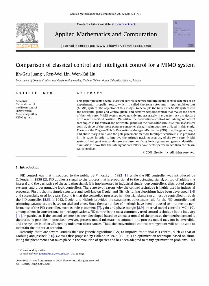
3.3. Gain–phase margin
Gain and phase margins are very important to analyze the control system in the frequency domain. It is applied to thecontrol system design by extending gain and phase margins such that the system can withstand greater changes in systemparameters before becoming unstable. Assume that the controller is the same as in (18), and assign phase margin and gainmargin to be /m and Am, respectively
Fig. 9.TRMS.
Fig. 10.TRMS.
GPðjxpÞ K þ j KTdxp �K
Tixp
� �� �¼ � 1
Am; ð26Þ
GPðjxgÞ K þ j KTdxg �K
Tixg
� �� �¼ �ej/m : ð27Þ
Let xp = axu, a 2 [0.5,2], where xu is the frequency limit and a = 1. When xp is chosen, control parameters can be solved by(26) and (27) as follows:
K ¼ Re�1
AmGPðjxpÞ
� �; ð28Þ
KTi¼ ðXPxg � XgxpÞ
xp
xg� xg
xp
� ��1
; ð29Þ
KTd ¼XP
xg� Xg
xp
� �xp
xg� xg
xp
� ��1
; ð30Þ
where XP ¼ Im �1AmGPðjxpÞ
� �, Xg ¼ Im �ej/m
GPðjxg Þ
� �, and xg needs to be satisfied by
Step response using the gain–phase margin rule in the horizontal plane, dot line is the desired yaw angle and solid line is the actual yaw angle of the
Step response using the gain–phase margin rule in the vertical plane, dot line is the desired pitch angle and solid line is the actual pitch angle of the
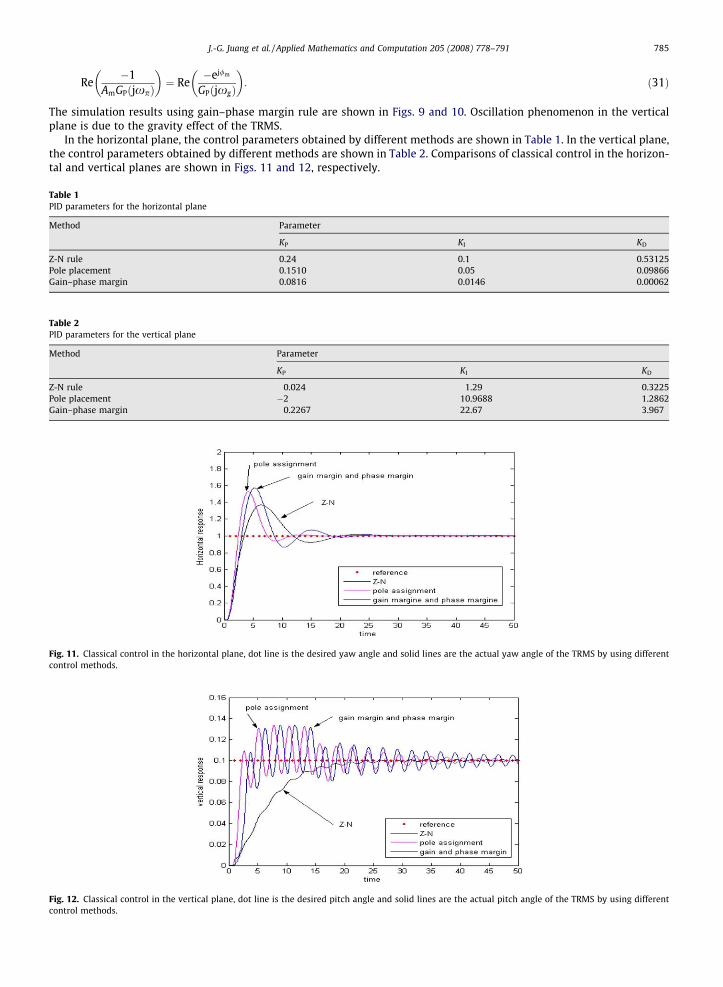
Fig. 11.control
Table 1PID par
Method
Z-N rulPole plaGain–p
Table 2PID par
Method
Z-N rulPole plaGain–p
Fig. 12.control
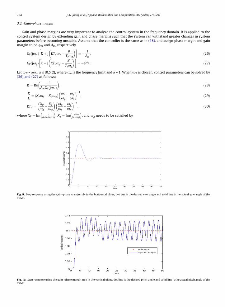
J.-G. Juang et al. / Applied Mathematics and Computation 205 (2008) 778–791 785
Re�1
AmGPðjxpÞ
� �¼ Re
�ej/m
GPðjxgÞ
� �: ð31Þ
The simulation results using gain–phase margin rule are shown in Figs. 9 and 10. Oscillation phenomenon in the verticalplane is due to the gravity effect of the TRMS.
In the horizontal plane, the control parameters obtained by different methods are shown in Table 1. In the vertical plane,the control parameters obtained by different methods are shown in Table 2. Comparisons of classical control in the horizon-tal and vertical planes are shown in Figs. 11 and 12, respectively.
Classical control in the horizontal plane, dot line is the desired yaw angle and solid lines are the actual yaw angle of the TRMS by using differentmethods.
ameters for the horizontal plane
Parameter
KP KI KD
e 0.24 0.1 0.53125cement 0.1510 0.05 0.09866
hase margin 0.0816 0.0146 0.00062
ameters for the vertical plane
Parameter
KP KI KD
e 0.024 1.29 0.3225cement �2 10.9688 1.2862
hase margin 0.2267 22.67 3.967
Classical control in the vertical plane, dot line is the desired pitch angle and solid lines are the actual pitch angle of the TRMS by using differentmethods.

786 J.-G. Juang et al. / Applied Mathematics and Computation 205 (2008) 778–791
4. Intelligent control of TRMS
Classical control systems are designed using models of physical systems. The selected mathematic model captures thedynamical behavior of interest, while control design techniques are applied to design the mathematical model by an appro-priate controller. The mathematical model of the system must be ‘‘simple enough” so that it can be analyzed with availablemathematical techniques, and must as well be ‘‘accurate enough” to describe the important aspects of the relevant dynam-ical behavior. It is quite clear that in controlling the systems, there are some requirements that cannot be addressed success-fully with the existing classical control theory. They mainly pertain to the issue of uncertainty because of the poor modelsand lack of knowledge, or because high-level models have been simplified to avoid excessive computational complexity.Intelligent control is thus needed in such cases. All control techniques that use various artificial intelligent computing ap-proaches like neural networks, fuzzy logic, machine learning, evolutionary computation, and genetic algorithms can beput into the class of intelligent control. In this paper, we utilize GA and fuzzy logic in the controller design.
4.1. Based on GA
The control system contains a PID controller. Control gains are obtained by a real-valued GA. The procedures of the GAoperations are described below:
Population: The GA does not work on a single individual but on a population P with p individuals, which undergoes anevolutionary process starting with the initial population P0. The simplest way to create P0 is to generate p strings or chro-mosome randomly. Each gene in the chromosome represents a specific parameter of the PID controller. The populationcan be expressed as
P ¼ ðx1; . . . ; xPÞ: ð32Þ
In the encoding process, we assign values for each gene within a specific range.Selection: The selection operator S selects an individual of the given population according to its fitness value. In this
paper, we chose the Roulette Wheel Selection as the selection process. This method is based on the ‘‘survival of the fittest”mechanism, in which individuals with higher fitness values have higher probabilities of producing an offspring. The proba-bility is,
PSi ¼fiPki¼1fi
ð33Þ
where fi is the fitness value of each individual, and k is the population size.Reproduction: This operator reproduces the selected individuals in the matting pool.
S0 ¼ R� S; ð34Þ
where S0 is new individual and S is the selected individual in the parent generation. R is the reproduction operator.Crossover: This operator exchanges the chromosome string of two selected individuals starting from a random index.
Here, we use the Adewuya crossover method for the crossover process. It is explained as follows:Assume that there are two selected individuals xpm and xpn in the parent generations:
xpm ¼ 1 2 3½ �; xpn ¼ 4 5 6½ �; ð35Þ
ais the crossover position, which is an integer generated within range [1,3] randomly; b is a real number generated withinrange [0,1] randomly.
When a = 2 and b = 0.3, the values in the parent generation xpm and xpn are 2 and 5. We substitute these parameters in (36)
xo1 ¼ ð1� bÞ � xpm þ b � xpn;
xo2 ¼ b � xpm þ ð1� bÞ � xpn:
ð36Þ
Then xo1 = 2.9, xo2 = 4.1. The genes in the left side of the crossover position are invariable, while the genes in the right side ofthe crossover position exchange with each other as shown in Fig. 13.
[ ]31 1opm xx =
[ ]64 2opn xx =
positioncrossover
positioncrossover
Fig. 13. Example of the Adewuya crossover law.

J.-G. Juang et al. / Applied Mathematics and Computation 205 (2008) 778–791 787
The individuals in the new generation are �xpm and �xpn, and the result is
Fig. 14.dash lin
Fig. 15.dash lin
�xpm ¼ 1 2:9 6½ �; �xpn ¼ 4 4:1 3½ � ð37Þ
Mutation: This mutation operator creates one new offspring individual for the new population by randomly mutating arandomly chosen gene of a selected individual. For example, there are p genes that represent p parameters in an individualP = [x1, . . . ,xk, . . . ,xp], and the kth parameter is in the mutation position within range UBk LBk½ �. The new gene is
xknew ¼ LBk þ r � ðUBk � LBkÞ; ð38Þ
where r is a real number within [0,1]. The individual after mutation is Pnew = [x1, . . . ,xknew, . . . ,xp].Fitness function: The fitness function f is used to direct the evolution in a certain direction. In fact, genetic algorithm is
merely a method of approximating the global maximum of f in the searching space of the chromosome strings. The actualinterpretation of this search space is packed into f and does not concern the algorithm itself. The fitness function is
Fitness Function ¼ qIITSE
; ð39Þ
where q is a positive number and IITSE is a system performance index, which is known as an integral of time multiplied by thesquared error criterion (ITSE) [27]. There are 10 individuals with three genes in the initial population. The crossover rate is0.8, and the mutation rate is 0.025. The objective parameters of GA are KP, KI, and KD within the range [0,1]. The simulationsare shown in Figs. 14 and 15. The control gains of the PID controller are obtained by the ITSE fitness function, which sets upthe rise time and overshoot as the criterion. Thus, the rise time and overshoot can be improved.
4.2. Based on fuzzy controller and GA
A fuzzy controller is applied to the TRMS control. The PID controller is replaced by the fuzzy controller as shown in Fig. 16.The structure of the fuzzy controller is shown in Fig. 17. In order to minimize the output error, the gain factors Se, Sce, Sse and
0 5 10 15 20 25 30 35 40 45 50-0.6
-0.4
-0.2
0
0.2
0.4
0.6
0.8
1
1.2horizontal simulation
Time (sec)
Deg
. (ra
d)
referencesystem outputcontrol signal
Step response using GA-PID controller in the horizontal plane, the desired yaw angle is set to 1 rad, solid line is the actual yaw angle of the TRMS,e is the control force to the TRMS.
0 5 10 15 20 25 30 35 40 45 50-0.6
-0.4
-0.2
0
0.2
0.4
0.6
0.8horizontal simulation
Time (sec)
Deg
. (ra
d)
re fe re nc esyst em out putco nt ro l si gnal
Step response using GA-PID controller in the vertical plane, the desired pitch angle is set to 0.2 rad, solid line is the actual pitch angle of the TRMS,e is the control force to the TRMS.

Fig. 16. Fuzzy controller in the TRMS.
1−Z
PIDu∧PIDuPIDu∧Δ∧Δe
∧e
Δe
eΔ
∧∧∧eeef ,,
∧ee
Se
Sce
Sse
FLC Su+ +
Fig. 17. Structure of fuzzy logic controller.
788 J.-G. Juang et al. / Applied Mathematics and Computation 205 (2008) 778–791
Su are tuned by GA, where e(n) = yd (n) � y(n), De(n) = e(n) � e(n � 1),P
e is the sum of errors, e ¼ See, De ¼ Scee,P
e ¼ SseP
eand uPID ¼ SuuPID. Define the linguistic variables that correspond to the input scaled variables e, De and
Pe as Ei;DEj;
PEk.
The indices i, j and k represent the linguistic values or fuzzy states of the input fuzzy variables and their ranges arei = 0,1,2,. . .,N1 � 1; j = 0,1,2, . . . ,N2 � 1; k = 0,1,2, . . . ,N3 � 1; where N1, N2 and N3 denote the total numbers of fuzzy statesassigned for each fuzzy variables. The fuzzy PID structure can be expressed as follows:
Fig. 18.dash lin
If e is Ei AND De is DEj ANDX
e isX
Ek
THEN DuPID is DUm;PID
ð40Þ
The final controller output can be expressed by
uPID ¼ Su
Xn
q¼0
DuPIDðqÞ: ð41Þ
In this work, we apply the Gaussian membership function for each control variable. The universe of discourse of each in-put and output variables is defined to be within the range [�1,1], uniformly portioned in seven membership functions, and
0 5 10 15 20 25 30 35 40 45 50-1
-0.5
0
0.5
1
1.5horizontal simulation
Time (sec)
Deg
. (ra
d)
referencesystem outputcontrol signal
Step response using fuzzy controller in the horizontal plane, the desired yaw angle is set to 1 rad, solid line is the actual yaw angle of the TRMS,e is the control force to the TRMS.
0 5 10 15 20 25 30 35 40 45 50-0.6
-0.4
-0.2
0
0.2
0.4
0.6
0.8
1
1.2
1.4horizontal simulation
Time (sec)
Deg
. (ra
d)
referencesystem outputcontrol signal
Fig. 19. Step response using fuzzy controller in the vertical plane, the desired pitch angle is set to 0.2 rad, solid line is the actual pitch angle of the TRMS,dash line is the control force to the TRMS.
J.-G. Juang et al. / Applied Mathematics and Computation 205 (2008) 778–791 789
placed with 50% overlap. The number of linguistic variables used for each e1, e2 and e3 is seven. The parameters of the fuzzycontroller are adjusted by GA. There are four scaling factors, Se, Sce, Sse and Su that need to be optimized within the range[0,2]. The crossover rate and mutation rate are 0.8 and 0.025, respectively. The computer simulations are shown in Figs.18 and 19. The PID controller is replaced by the fuzzy controller, which is based on the IF THEN rule to generate the controlforce for the TRMS. Thus, the control forces in Figs. 18 and 19 oscillate in the beginning for a short time, like the bang–bangcontrol.
Fig. 20. Fuzzy compensator and PID controller in the TRMS.
0 5 10 15 20 25 30 35 40 45 50-1
-0.5
0
0.5
1
1.5horizontal simulation
Time (sec)
Deg
. (ra
d)
referencesystem outputcontrol signal
Fig. 21. Step response using fuzzy compensator and PID controller in the horizontal plane, the desired yaw angle is set to 1 rad, solid line is the actual yawangle of the TRMS, dash line is the control force to the TRMS.
0 5 10 15 20 25 30 35 40 45 50-0.6
-0.4
-0.2
0
0.2
0.4
0.6
0.8
1horizontal simulation
Time (sec)
Deg
. (ra
d)
referencesystem outputcontrol signal
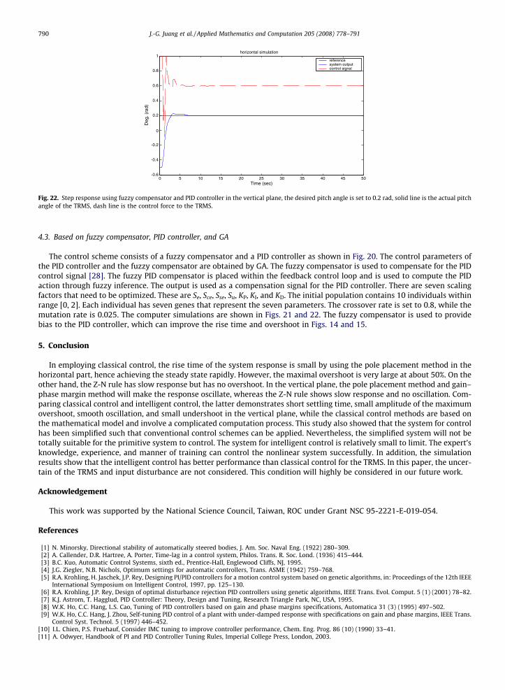
Fig. 22. Step response using fuzzy compensator and PID controller in the vertical plane, the desired pitch angle is set to 0.2 rad, solid line is the actual pitchangle of the TRMS, dash line is the control force to the TRMS.
790 J.-G. Juang et al. / Applied Mathematics and Computation 205 (2008) 778–791
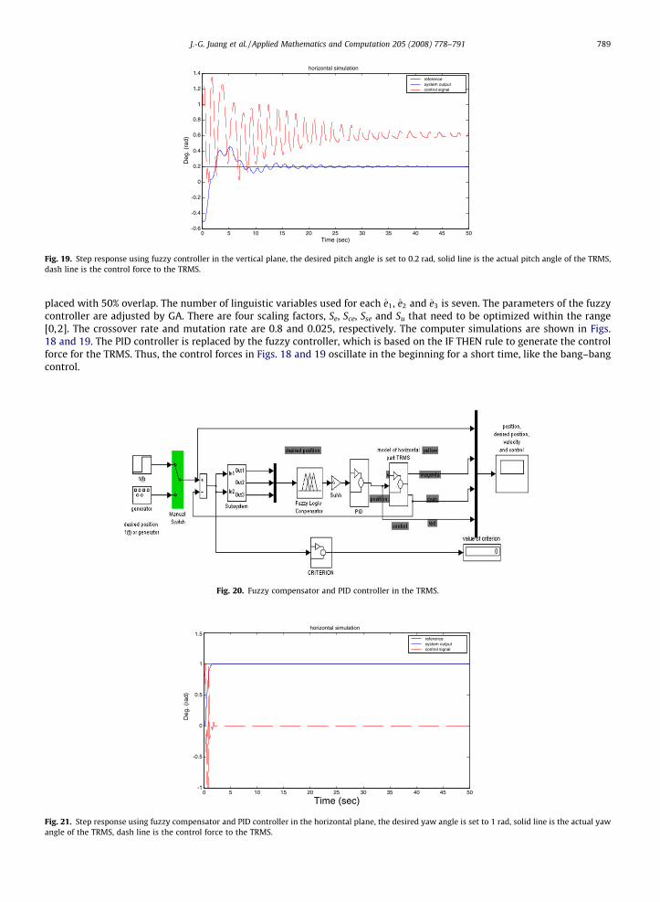
4.3. Based on fuzzy compensator, PID controller, and GA
The control scheme consists of a fuzzy compensator and a PID controller as shown in Fig. 20. The control parameters ofthe PID controller and the fuzzy compensator are obtained by GA. The fuzzy compensator is used to compensate for the PIDcontrol signal [28]. The fuzzy PID compensator is placed within the feedback control loop and is used to compute the PIDaction through fuzzy inference. The output is used as a compensation signal for the PID controller. There are seven scalingfactors that need to be optimized. These are Se, Sce, Sse, Su, KP, KI, and KD. The initial population contains 10 individuals withinrange [0, 2]. Each individual has seven genes that represent the seven parameters. The crossover rate is set to 0.8, while themutation rate is 0.025. The computer simulations are shown in Figs. 21 and 22. The fuzzy compensator is used to providebias to the PID controller, which can improve the rise time and overshoot in Figs. 14 and 15.
5. Conclusion
In employing classical control, the rise time of the system response is small by using the pole placement method in thehorizontal part, hence achieving the steady state rapidly. However, the maximal overshoot is very large at about 50%. On theother hand, the Z-N rule has slow response but has no overshoot. In the vertical plane, the pole placement method and gain–phase margin method will make the response oscillate, whereas the Z-N rule shows slow response and no oscillation. Com-paring classical control and intelligent control, the latter demonstrates short settling time, small amplitude of the maximumovershoot, smooth oscillation, and small undershoot in the vertical plane, while the classical control methods are based onthe mathematical model and involve a complicated computation process. This study also showed that the system for controlhas been simplified such that conventional control schemes can be applied. Nevertheless, the simplified system will not betotally suitable for the primitive system to control. The system for intelligent control is relatively small to limit. The expert’sknowledge, experience, and manner of training can control the nonlinear system successfully. In addition, the simulationresults show that the intelligent control has better performance than classical control for the TRMS. In this paper, the uncer-tain of the TRMS and input disturbance are not considered. This condition will highly be considered in our future work.
Acknowledgement
This work was supported by the National Science Council, Taiwan, ROC under Grant NSC 95-2221-E-019-054.
References
[1] N. Minorsky, Directional stability of automatically steered bodies, J. Am. Soc. Naval Eng. (1922) 280–309.[2] A. Callender, D.R. Hartree, A. Porter, Time-lag in a control system, Philos. Trans. R. Soc. Lond. (1936) 415–444.[3] B.C. Kuo, Automatic Control Systems, sixth ed., Prentice-Hall, Englewood Cliffs, NJ, 1995.[4] J.G. Ziegler, N.B. Nichols, Optimum settings for automatic controllers, Trans. ASME (1942) 759–768.[5] R.A. Krohling, H. Jaschek, J.P. Rey, Designing PI/PID controllers for a motion control system based on genetic algorithms, in: Proceedings of the 12th IEEE
International Symposium on Intelligent Control, 1997, pp. 125–130.[6] R.A. Krohling, J.P. Rey, Design of optimal disturbance rejection PID controllers using genetic algorithms, IEEE Trans. Evol. Comput. 5 (1) (2001) 78–82.[7] K.J. Astrom, T. Hagglud, PID Controller: Theory, Design and Tuning, Research Triangle Park, NC, USA, 1995.[8] W.K. Ho, C.C. Hang, L.S. Cao, Tuning of PID controllers based on gain and phase margins specifications, Automatica 31 (3) (1995) 497–502.[9] W.K. Ho, C.C. Hang, J. Zhou, Self-tuning PID control of a plant with under-damped response with specifications on gain and phase margins, IEEE Trans.
Control Syst. Technol. 5 (1997) 446–452.[10] I.L. Chien, P.S. Fruehauf, Consider IMC tuning to improve controller performance, Chem. Eng. Prog. 86 (10) (1990) 33–41.[11] A. Odwyer, Handbook of PI and PID Controller Tuning Rules, Imperial College Press, London, 2003.

J.-G. Juang et al. / Applied Mathematics and Computation 205 (2008) 778–791 791
[12] J.H. Holland, Adaptation in Natural and Artificial System, University of Michigan Press, 1975.[13] R. Subbu, K. Goebel, D.K. Frederick, Evolutionary design and optimization of aircraft engine controllers, IEEE Trans. Syst. Man Cybernet. Pt. C 35 (4)
(2005) 554–565.[14] J.G. Juang, B.S. Lin, Nonlinear system identification by evolutionary computation and recursive estimation method, in: Proceedings of American Control
Conference, 2005, pp. 5073–5078.[15] J.G. Juang, H.K. Chiou, Hybrid RNN-GA controller for ALS in wind shear condition, in: Proceedings of IEEE International Conference on Systems, Man &
Cybernetics, 2006, pp. 675–680.[16] H.-J. Cho, K.-B. Cho, B.-I. Wang, Automatic rule generation using genetic algorithms for fuzzy-PID hybrid control, in: Proceedings of IEEE International
Symposium on Intelligent Control, 1996, pp. 271–276.[17] B. Hu, G.K.I. Mann, G. Raymond, New methodology for analytical and optimal design of fuzzy PID controllers, Proc. IEEE Trans. Fuzzy Syst. 7 (5) (1999)
521–539.[18] Y.-S. Zhou, L.-Y. Lai, Optimal design for fuzzy controllers by genetic algorithms, IEEE Trans. Ind. Appl. 36 (1) (2000) 93–97.[19] K. Belarbi, F. Titel, Genetic algorithm for the design of a class of fuzzy controllers: an alternative, IEEE Trans. Fuzzy Syst. 8 (3) (2000) 398–405.[20] L.A. Zadeh, Fuzzy sets, Inform. Control 8 (1965) 338–352.[21] J.T. Alander, An indexed bibliography of genetic algorithms with fuzzy logic, in: W. Pedrycz (Ed.), Fuzzy Evolutionary Computation, Kluwer Academic,
Boston, 1997, pp. 299–318.[22] C.L. Karr, Genetic algorithm for fuzzy controllers, AI Expert 6 (1991) 26–33.[23] A. Bonarini, Evolutionary learning of fuzzy rules: competition and cooperation, in: W. Pedrycz (Ed.), Fuzzy Modelling: Paradigms and Practice, Kluwer
Academic Press, Norwell, MA, 1996, pp. 265–284.[24] S.F. Lee, H.C. Lu, T.H. Hung, Optimal design GA-based fuzzy PID controllers, in: Proceedings of IEEE International Conference on SMC, vol. 2, 2002, pp.
215–220.[25] Feedback Co, Twin Rotor MIMO System 33-220 User Manual, 3-000M5, 1998.[26] W.K. Liu, Applications of hybrid fuzzy-GA controller and FPGA chip to TRMS, M.S. Thesis, Department of Communications and Guidance Engineering,
National Taiwan Ocean University, 2005.[27] J.G. Juang, K.T. Tu, W.K. Liu, Hybrid intelligent PID control for MIMO system, Lect. Notes Comput. Sci. 4234 (2006) 654–663.[28] J.G. Juang, W.K. Liu, Fuzzy compensator using RGA for TRMS control, Lect. Notes Artif. Intell. 4114 (2006) 120–126.