1-s2.0-S0022460X15001546-main

Contents lists available at ScienceDirect

Journal of Sound and Vibration

Journal of Sound and Vibration ] (]]]]) ]]]–]]]

http://d0022-46

n CorrE-m

PleasVibra

journal homepage: www.elsevier.com/locate/jsvi

Dynamic stiffness formulation for free orthotropic plates

O. Ghorbel a, J.B. Casimir b,n, L. Hammami a, I. Tawfiq b, M. Haddar a

a Ecole Nationale d'Ingénieurs de Sfax, Université de Sfax, Unité de Mécanique, Modélisation et Production, Route Soukra Km 3.5,BP 1173 3038 Sfax, Tunisiab Institut Supérieur de Mécanique de Paris, LISMMA-Quartz, 3 rue Fernand Hainaut 93407 Saint-Ouen, France

a r t i c l e i n f o

Article history:Received 17 August 2014Received in revised form23 January 2015Accepted 9 February 2015
Handling Editor: M.P. Cartmell
of the symmetry and Gorman type decomposition of the free boundary conditions.

x.doi.org/10.1016/j.jsv.2015.02.0200X/& 2015 Elsevier Ltd. All rights reserved.

esponding author.ail address: [email protected]

e cite this article as: O. Ghorbel, et ation (2015), http://dx.doi.org/10.1016

a b s t r a c t

This paper presents a procedure for developing the dynamic stiffness matrix of a freeorthotropic Kirchhoff plate. The dynamic stiffness matrix is computed for free edgeboundary conditions of the plate that allow assembly procedures. The method is based ona strong formulation of Kirchhoff plate equations and series solutions, taking advantage

The performances of the so-called Dynamic Stiffness Method (DSM) are evaluated bycomparing the harmonic responses of an orthotropic Kirchhoff plate with those obtainedfrom the Finite Element Method using four noded quadrilateral elements.

& 2015 Elsevier Ltd. All rights reserved.

1. Introduction

For many years, the subject of structural vibration has attracted considerable attention from researchers and engineers inthe aerospace, shipbuilding and other industries. As composite materials are now increasingly used in these industries, thevibrations of mechanical structures made of such materials must be investigated in detail. The response of structures subjectedto harmonic loads is one of the main dynamic problems researchers must tackle and several methods have been developed tosolve the problem. A popular method is the Finite Element Method (FEM) which has led to the development of isotropic andanisotropic beam, plate and shell elements [1]. FEM formulations of anisotropic and multilayered plates have been widelyinvestigated since the beginning of the 1970s. Prior and Barker [2] developed one of the first finite element models forlaminates including transverse shear deformations. Later, many other publications presented new finite element formulationsfor thick and thin multilayer laminated plates, for example [3–5]. Today, the development of finite elements devoted tocomposite structures is still in progress [6,7]. The Boundary Element Method (BEM) has also proved to be efficient forinvestigating orthotropic plate vibration problems in particular. For example, Albuquerque et al. [8] used the BEM for analyzingsimply supported orthotropic Kirchoff plates as well as cross-ply laminated plates with simply supported and clamped edges.However, the main disadvantage of BEM, FEM and other approximate methods is that they are essentially based on thediscretization of the structure's geometry. In fact, the mesh of the structure has considerable influence on the precision of theresults, especially in the high frequency range. Meshless methods are often used to overcome this limitation but they are oftenrestricted to very specific boundary conditions and are also unsuitable for assembly procedures. Significant research has beendevoted to developing simply supported and built-in boundary conditions for plates. Thinh et al. [9] used the DynamicStiffness Method for orthotropic plates on simply supported multi-section Winkler-type and Pasternak-type elastic

r (J.B. Casimir).

l., Dynamic stiffness formulation for free orthotropic plates, Journal of Sound and

/j.jsv.2015.02.020i

www.sciencedirect.com/science/journal/0022460X

www.elsevier.com/locate/jsvi

http://dx.doi.org/10.1016/j.jsv.2015.02.020



mailto:[email protected]





O. Ghorbel et al. / Journal of Sound and Vibration ] (]]]]) ]]]–]]]2

foundations. Dozio studied the free vibration of cross-ply laminated plates with two simply supported opposite edges usingfundamental nuclei [10] and Levy methods [11]. To solve similar problems Thai and Kim [12] employed Levy series and refinedplate theory for a simply supported boundary condition with two opposite edges and changed the boundary conditions of theother edges using the Mindlin theory for the free vibration analysis of orthotropic plates. Furthermore, Leissa [13] presentedthe analytical solution of an orthotropic Kirchhoff plate in which he fixed the two edges for a simply supported configurationand changed the boundary conditions with the other edges.

Assembling two or more plates requires free edge boundary conditions. Levy series displacement solutions based ontrigonometric functions cannot directly satisfy these boundary conditions where equilibrating forces vanish. Gorman [14]proposed a solution for plates where all the edges are free. He used a block decomposition to determine the naturalfrequencies for free plates. Casimir et al. [15] used symmetry consideration and Gorman's decomposition method to arrive atan exact solution based on Levy's series, and developed the dynamic stiffness matrix of a free edge isotropic Kirchoff plate.This approach allowed them to extend the so-called Dynamic Stiffness Method (DSM) to plate elements.

DSM is particularly efficient for analyzing and studying the harmonic response of complex structures [16–18]. Theabsence of discretization errors makes it possible to obtain precise results and considerably reduce computation time. Thismethod is based on exact solutions of elastodynamic equations in the harmonic region. The dynamic stiffness matrix KðωÞ isessentially a function of a given circular frequency ω. This matrix links the amplitudes of displacements U and externalforces F acting on the boundaries of the structural element to give

KðωÞU¼ F (1)

Various elements have been developed using DSM which include beams [19–21], rings [22], laminated composite plates[23], shells [24–26] and the method has been implemented in several computer programs [27–30], but the element librariesare rather limited. Enriching software development using the DSM is one of the objectives of this paper.

The main aim of this paper is, of course, to present the methodology for developing the dynamic stiffness matrix of anorthotropic Kirchhoff plate for free edge boundary conditions. In order to achieve this, Gorman's decompositions of foursymmetry contributions are used and Levy type solutions are obtained for the free edge conditions. Therefore, the dynamicstiffness matrix is obtained by superposing all of the symmetry contributions. This dynamic stiffness matrix is used tocompute the harmonic response of orthotropic plates and the results obtained from the theory are validated using thetraditional or conventional finite element method.

2. Kirchhoff's orthotropic plate equations

2.1. Geometry

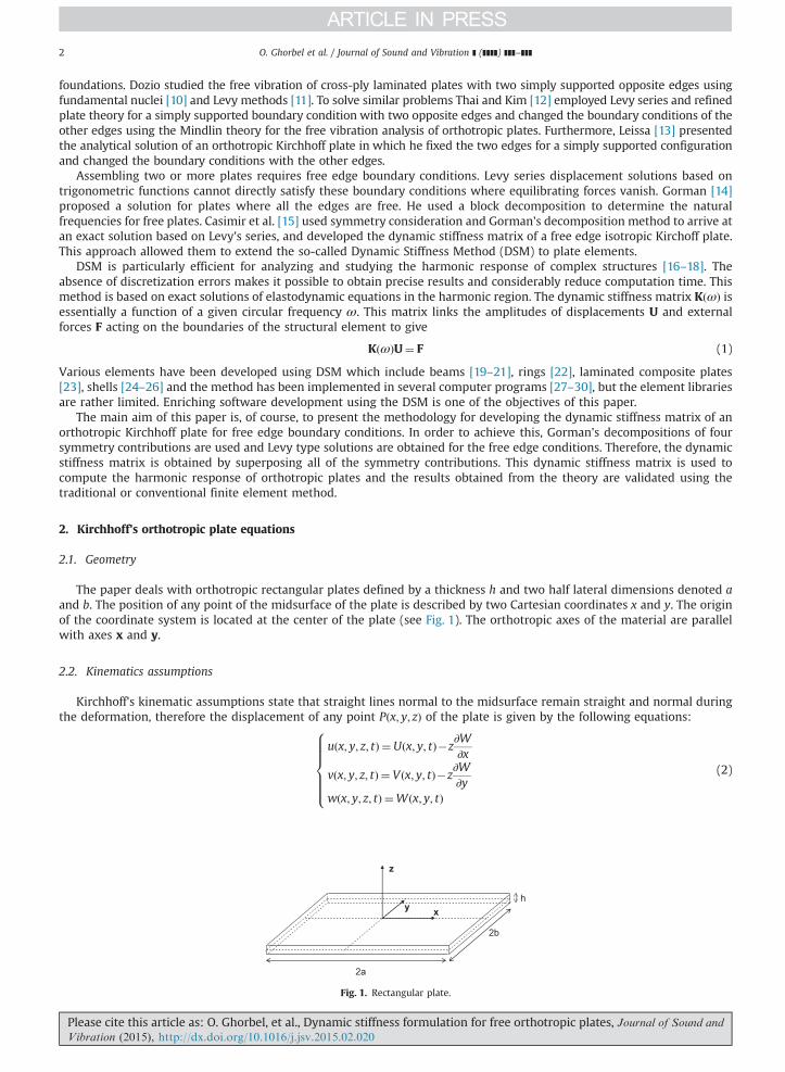
The paper deals with orthotropic rectangular plates defined by a thickness h and two half lateral dimensions denoted aand b. The position of any point of the midsurface of the plate is described by two Cartesian coordinates x and y. The originof the coordinate system is located at the center of the plate (see Fig. 1). The orthotropic axes of the material are parallelwith axes x and y.

2.2. Kinematics assumptions

Kirchhoff's kinematic assumptions state that straight lines normal to the midsurface remain straight and normal duringthe deformation, therefore the displacement of any point Pðx; y; zÞ of the plate is given by the following equations:

u x; y; z; tð Þ ¼U x; y; tð Þ�z∂W∂x

v x; y; z; tð Þ ¼ V x; y; tð Þ�z∂W∂y

wðx; y; z; tÞ ¼Wðx; y; tÞ

8>>>>><>>>>>:

(2)

xy

z

2b

2a

h

Fig. 1. Rectangular plate.

Please cite this article as: O. Ghorbel, et al., Dynamic stiffness formulation for free orthotropic plates, Journal of Sound and

Vibration (2015), http://dx.doi.org/10.1016/j.jsv.2015.02.020i




O. Ghorbel et al. / Journal of Sound and Vibration ] (]]]]) ]]]–]]] 3

where u, v, w are displacements of P along axes x, y and z, respectively. U, U,W are displacements of the projection of point Pon the midsurface of the plate.

The rotations of the midsurface are denoted βx and βy, they are given by the following equations:

βx ¼ �∂W∂x

βy ¼ �∂W∂y

8>><>>: (3)

2.3. Constitutive relations

The constitutive relations of the orthotropic plates are obtained by considering the plane stress assumption. In theorthotropic axes (1,2,3), these relations are given by the following equations:

σ11 ¼Q11ϵ11þQ12ϵ22σ22 ¼Q12ϵ11þQ22ϵ22σ12 ¼Q66ϵ12

8><>: (4)

where σ11, σ22, σ12 are the components of the Cauchy stress tensor and ϵ11, ϵ22, ϵ12 are the components of the small straintensor. Material constants Qij are given by the following equations:

Q11 ¼E1

1�ν12ν21

Q22 ¼E2

1�ν12ν21

Q12 ¼ν12E2

1�ν12ν21¼ ν21E11�ν12ν21

Q66 ¼ G12

8>>>>>>>>><>>>>>>>>>:

(5)

where E1, E2 are Young's moduli along the orthotropic directions 1 and 2, respectively, ν12, ν21 are major and minor Poisson'sratios and G12 is the shear modulus.

The 3D plate problem is essentially reduced to a 2D problem by integrating the stresses along the thickness of the plate.For a single layer orthotropic plate with a constant thickness h, in-plane and out-of-plane displacements are uncoupled. Theforces associated with out-of-plane displacements are as follows:

�

PV

Transverse shear forces

Tx ¼Z h=2

�h=2σxz dz; Ty ¼

Z h=2

�h=2σyz dz (6)

�
Bending moments
Mx ¼Z h=2

�h=2zσxx dz; My ¼

Z h=2

�h=2zσyy dz (7)

�
Twisting moment
Mxy ¼Z h=2

�h=2zσxy dz (8)

The small strains, obtained from the displacement field (Eq. (2)), are introduced in the constitutive equations (Eq. (4)) toobtain stress/displacement relationships. Then, internal force/displacement relationships are obtained from internal forcedefinitions. In the case of plates, for which the orientation of the constitutive material is such that orthotropic axes 1 and 2

lease cite this article as: O. Ghorbel, et al., Dynamic stiffness formulation for free orthotropic plates, Journal of Sound and

ibration (2015), http://dx.doi.org/10.1016/j.jsv.2015.02.020i





are equal to axes x and y, respectively, we obtain the following equations:

Mx ¼ �h3

12Q11

∂2W∂x2

�h3

12Q12

∂2W∂y2

My ¼ �h3

12Q12

∂2W∂x2

�h3

12Q22

∂2W∂y2

Mxy ¼ �2h3

12Q66

∂2W∂x∂y

8>>>>>>>>>><>>>>>>>>>>:

(9)

2.4. Equations of motion

Hamilton's principle gives the well-known equations of motion for plates as follows:

∂2Mx

∂x2þ2

∂2Mxy

∂x∂yþ∂2My

∂y2¼ ρh

∂2W∂t2

(10)

where ρ is the mass density of the material.By introducing the constitutive equations (9) in Eq. (10), the following governing differential equation of an orthotropic

plate in free vibration is obtained:

Dx∂4W∂x4

þDxy∂4W∂x2∂y2

þDy∂4W∂y4

¼ ρh∂2W∂t2

(11)

where

Dx ¼ �h3

12Q11

Dxy ¼ �h3

6Q12�4

h3

12Q66

Dy ¼ �h3

12Q22

8>>>>>>>><>>>>>>>>:

(12)

In the case of harmonic oscillation, time t can be eliminated. Thus by using Eq. (13), Eq. (11) becomes Eq. (14) as shownbelow:

Wðx; y; tÞ ¼W0ðx; yÞeiωt (13)

Dx∂4W0

∂x4þDxy

∂4W0

∂x2∂y2þDy

∂4W0

∂y4¼ �ρhω2W0 (14)

whereW0ðx; yÞ is the amplitude of the harmonic out-of-plane displacement of the point lying on the midsurface at position (x,y).

2.5. Boundary conditions

Free edge boundary conditions are considered to solve the strong formulation of the dynamic problem. These boundaryconditions describe external transverse forces and bending moments along the edges of the plate. The external transverseforce acting along the edge whose normal vector is n is denoted Fn. The external moments acting along this edge aredenoted Mn and Mns. Kirchhoff's assumptions and Hamilton's principle lead to defining boundary conditions in terms ofinternal forces. They are given by the following equations:

Tnþ∂Mns

∂s¼ Fz

Mn ¼Mn

8<: (15)

where Fz ¼F nþ∂Mns=∂s. Letters n and s designate the spatial coordinates x or y along the edge considered.

3. Dynamic stiffness matrix for free orthotropic plates

The Dynamic Stiffness Method is based on the derivation of the dynamic stiffness matrix. This matrix is obtained withoutany discretization of the plate. Strong solutions of the harmonic problem described by Eq. (14) are used to determine therelationships between external forces and edge displacements for a given circular frequency ω. In the case of two-dimensional elements such as plates or shells, the external forces and displacements of the edges are continuous functions.Numerical relationships between these functions require using of a projection functional basis defined on each free edge.The matrix relation sought is related to the projections of force and displacement functions on each edge functional basis.







The dynamic stiffness matrix is calculated for free edge boundary conditions. Assembling procedures between two platescan only be performed with free edge boundary conditions. Other boundary conditions can be obtained from this generalfree edge case by eliminating lines and columns in the dynamic stiffness matrix or using other penalty methods. Thedifficulty of dealing with these kind of boundary conditions is overcome by introducing four symmetry contributions of thetotal displacement and the Gorman boundary condition decomposition method [14], as explained hereafter.

3.1. Strong solutions

Strong solutions are obtained by splitting the displacement into four symmetry contributions. This decomposition isgiven by the following equation:

W0ðξ;ηÞ ¼WSSðξ;ηÞþWAAðξ;ηÞþWSAðξ;ηÞþWASðξ;ηÞ (16)

where ξ and η are non-dimensional spatial coordinates

ξ¼ x=a; η¼ y=b (17)

WSS is the doubly symmetric contribution, WAA is the doubly antisymmetric contribution, WSA is the symmetric aboutX-antisymmetric about Y contribution and WAS is antisymmetric about X-symmetric about Y contribution. For example, WSA

contribution is such that WSAðx; yÞ ¼WSAð�x; yÞ and WSAðx; yÞ ¼ �WSAðx; �yÞ.Using Levy series allows reducing the partial differential equation (Eq. (14)) to ordinary differential equations whose

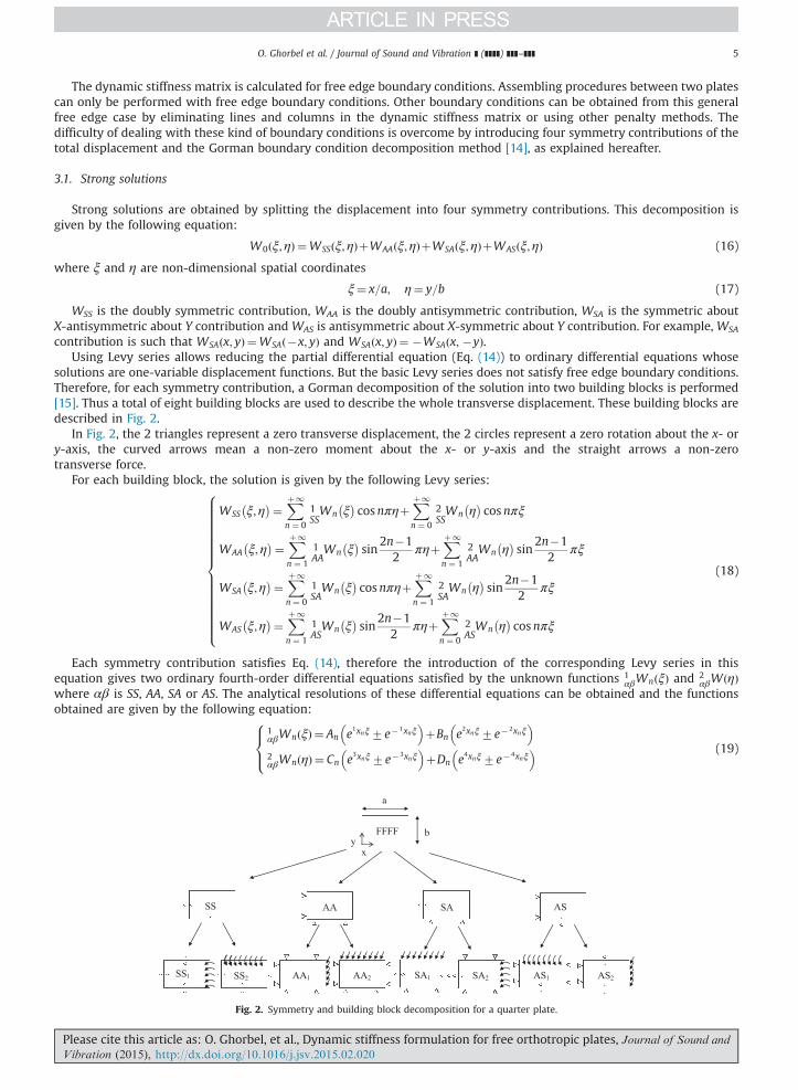
solutions are one-variable displacement functions. But the basic Levy series does not satisfy free edge boundary conditions.Therefore, for each symmetry contribution, a Gorman decomposition of the solution into two building blocks is performed[15]. Thus a total of eight building blocks are used to describe the whole transverse displacement. These building blocks aredescribed in Fig. 2.

In Fig. 2, the 2 triangles represent a zero transverse displacement, the 2 circles represent a zero rotation about the x- ory-axis, the curved arrows mean a non-zero moment about the x- or y-axis and the straight arrows a non-zerotransverse force.

For each building block, the solution is given by the following Levy series:

WSS ξ;η� �¼ Xþ1

n ¼ 0

1SSWn ξ� �

cosnπηþXþ1

n ¼ 0

2SSWn η� �

cosnπξ

WAA ξ;η� �¼ Xþ1

n ¼ 1

1AAWn ξ� �

sin2n�1

2πηþ

Xþ1

n ¼ 1

2AAWn η� �

sin2n�1

2πξ

WSA ξ;η� �¼ Xþ1

n ¼ 0

1SAWn ξ� �

cosnπηþXþ1

n ¼ 1

2SAWn η� �

sin2n�1

2πξ

WAS ξ;η� �¼ Xþ1

n ¼ 1

1ASWn ξ� �

sin2n�1

2πηþ

Xþ1

n ¼ 0

2ASWn η� �

cosnπξ

8>>>>>>>>>>>>>>>><>>>>>>>>>>>>>>>>:

(18)

Each symmetry contribution satisfies Eq. (14), therefore the introduction of the corresponding Levy series in thisequation gives two ordinary fourth-order differential equations satisfied by the unknown functions 1

αβWnðξÞ and 2αβWðηÞ

where αβ is SS, AA, SA or AS. The analytical resolutions of these differential equations can be obtained and the functionsobtained are given by the following equation:

1αβWnðξÞ ¼ An e

1xnξ7e� 1xnξ� �

þBn e2xnξ7e� 2xnξ

� �2αβWnðηÞ ¼ Cn e

3xnξ7e� 3xnξ� �

þDn e4xnξ7e� 4xnξ

� �8><>: (19)

xy

a

bFFFF

SS AA SA AS

SS1 SS2 AA1 AA2 SA1 SA2 AS1 AS2

Fig. 2. Symmetry and building block decomposition for a quarter plate.







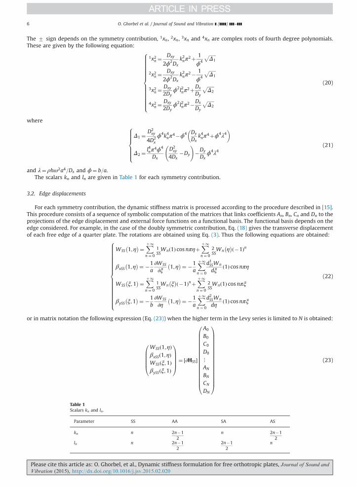
The 7 sign depends on the symmetry contribution, 1xn, 2xn, 3xn and 4xn are complex roots of fourth degree polynomials.These are given by the following equation:

1x2n ¼Dxy

2ϕ2Dx

k2nπ2þ 1

ϕ4

ffiffiffiffiffiffiΔ1

p2x2n ¼

Dxy

2ϕ2Dx

k2nπ2� 1

ϕ4


p3x2n ¼

Dxy

2Dyϕ2l2nπ

2þDx

Dy


p4x2n ¼

Dxy

2Dyϕ2l2nπ

2�Dx

Dy


p

8>>>>>>>>>>>>><>>>>>>>>>>>>>:

(20)

where

Δ1 ¼D2xy

4D2x

ϕ4k4nπ4�ϕ4 Dy

Dxk4nπ

4þϕ4λ4� �

Δ2 ¼l4nπ

4ϕ4

Dx

D2xy

4Dx�Dy

!�Dy

Dxϕ4λ4

8>>>>><>>>>>:

(21)

and λ¼ ρhω2a4=Dx and ϕ¼ b=a.The scalars kn and ln are given in Table 1 for each symmetry contribution.

3.2. Edge displacements

For each symmetry contribution, the dynamic stiffness matrix is processed according to the procedure described in [15].This procedure consists of a sequence of symbolic computation of the matrices that links coefficients An, Bn, Cn and Dn to theprojections of the edge displacement and external force functions on a functional basis. The functional basis depends on theedge considered. For example, in the case of the doubly symmetric contribution, Eq. (18) gives the transverse displacementof each free edge of a quarter plate. The rotations are obtained using Eq. (3). Thus the following equations are obtained:

WSS 1;η� �¼ Xþ1

n ¼ 0

1SSWn 1ð Þ cosnπηþ

Xþ1

n ¼ 0

2SSWn η� � �1ð Þn

βxSS 1;η� �¼ �1

a∂WSS

∂ξ1;η� �¼ �1

a

Xþ1

n ¼ 0

d1SSWn

dξ1ð Þ cosnπη

WSS ξ;1� �¼ Xþ1

n ¼ 0

1SSWn ξ� � �1ð Þnþ

Xþ1

n ¼ 0

2SSWn 1ð Þ cosnπξ

βySS ξ;1� �¼ �1

b∂WSS

∂η1;η� �¼ �1

a

Xþ1

n ¼ 0

d2SSWn

dη1ð Þ cosnπξ

8>>>>>>>>>>>>>>>><>>>>>>>>>>>>>>>>:

(22)

or in matrix notation the following expression (Eq. (23)) when the higher term in the Levy series is limited to N is obtained:

WSSð1;ηÞβxSSð1;ηÞWSSðξ;1ÞβySSðξ;1Þ

0BBBB@

1CCCCA¼ ½∂HSS�

A0

B0

C0

D0

⋮AN

BN

CN

DN

0BBBBBBBBBBBBBBBB@

1CCCCCCCCCCCCCCCCA

(23)

Table 1Scalars kn and ln.

Parameter SS AA SA AS

kn n 2n�12

n 2n�12

ln n 2n�12

2n�12

n







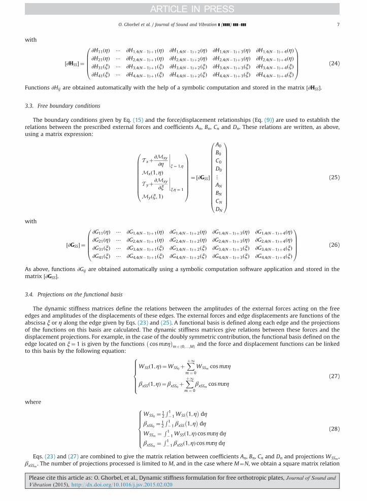
with

½∂HSS� ¼

∂H11ðηÞ ⋯ ∂H1;4ðN�1Þþ1ðηÞ ∂H1;4ðN�1Þþ2ðηÞ ∂H1;4ðN�1Þþ3ðηÞ ∂H1;4ðN�1Þþ4ðηÞ∂H21ðηÞ ⋯ ∂H2;4ðN�1Þþ1ðηÞ ∂H2;4ðN�1Þþ2ðηÞ ∂H2;4ðN�1Þþ3ðηÞ ∂H2;4ðN�1Þþ4ðηÞ∂H31ðξÞ ⋯ ∂H3;4ðN�1Þþ1ðξÞ ∂H3;4ðN�1Þþ2ðξÞ ∂H3;4ðN�1Þþ3ðξÞ ∂H3;4ðN�1Þþ4ðξÞ∂H41ðξÞ ⋯ ∂H4;4ðN�1Þþ1ðξÞ ∂H4;4ðN�1Þþ2ðξÞ ∂H4;4ðN�1Þþ3ðξÞ ∂H4;4ðN�1Þþ4ðξÞ

0BBBB@

1CCCCA (24)

Functions ∂Hij are obtained automatically with the help of a symbolic computation and stored in the matrix ½∂HSS�.

3.3. Free boundary conditions

The boundary conditions given by Eq. (15) and the force/displacement relationships (Eq. (9)) are used to establish therelations between the prescribed external forces and coefficients An, Bn, Cn and Dn. These relations are written, as above,using a matrix expression:

T xþ∂Mxy

∂η

ξ ¼ 1;η

Mxð1;ηÞ

T yþ∂Mxy

∂ξ

ξ;η ¼ 1

Myðξ;1Þ

0BBBBBBBBB@

1CCCCCCCCCA

¼ ∂GSS½ �

A0

B0

C0

D0

⋮AN

BN

CN

DN

0BBBBBBBBBBBBBBBB@

1CCCCCCCCCCCCCCCCA

(25)

with

½∂GSS� ¼

∂G11ðηÞ ⋯ ∂G1;4ðN�1Þþ1ðηÞ ∂G1;4ðN�1Þþ2ðηÞ ∂G1;4ðN�1Þþ3ðηÞ ∂G1;4ðN�1Þþ4ðηÞ∂G21ðηÞ ⋯ ∂G2;4ðN�1Þþ1ðηÞ ∂G2;4ðN�1Þþ2ðηÞ ∂G2;4ðN�1Þþ3ðηÞ ∂G2;4ðN�1Þþ4ðηÞ∂G31ðξÞ ⋯ ∂G3;4ðN�1Þþ1ðξÞ ∂G3;4ðN�1Þþ2ðξÞ ∂G3;4ðN�1Þþ3ðξÞ ∂G3;4ðN�1Þþ4ðξÞ∂G41ðξÞ ⋯ ∂G4;4ðN�1Þþ1ðξÞ ∂G4;4ðN�1Þþ2ðξÞ ∂G4;4ðN�1Þþ3ðξÞ ∂G4;4ðN�1Þþ4ðξÞ

0BBBB@

1CCCCA (26)

As above, functions ∂Gij are obtained automatically using a symbolic computation software application and stored in thematrix ½∂GSS�.

3.4. Projections on the functional basis

The dynamic stiffness matrices define the relations between the amplitudes of the external forces acting on the freeedges and amplitudes of the displacements of these edges. The external forces and edge displacements are functions of theabscissa ξ or η along the edge given by Eqs. (23) and (25). A functional basis is defined along each edge and the projectionsof the functions on this basis are calculated. The dynamic stiffness matrices give relations between these forces and thedisplacement projections. For example, in the case of the doubly symmetric contribution, the functional basis defined on theedge located on ξ¼ 1 is given by the functions cosmπη

� �mA f0;…;Mg and the force and displacement functions can be linked

to this basis by the following equation:

WSSð1;ηÞ ¼WSS0 þXþ1

m ¼ 0

WSSm cosmπη

βxSSð1;ηÞ ¼ βxSS0 þXþ1

m ¼ 0

βxSSm cosmπη

8>>>>><>>>>>:

(27)

where

WSS0 ¼ 12

R 1�1 WSS 1;η

� �dη

βxSS0 ¼ 12

R 1�1 βxSS 1;η

� �dη

WSSm ¼ R 1�1 WSSð1;ηÞ cosmπη dη

βxSSm ¼ R 1�1 βxSSð1;ηÞ cosmπη dη

8>>>>>><>>>>>>:

(28)

Eqs. (23) and (27) are combined to give the matrix relation between coefficients An, Bn, Cn and Dn and projections WSSm ,βxSSm . The number of projections processed is limited to M, and in the case where M¼N, we obtain a square matrix relation







(see the following equation):

1SSW01SSβx02SSW02SSβy0

⋮1SSWM1SSβxM2SSWM2SSβyM

0BBBBBBBBBBBBBBBBB@

1CCCCCCCCCCCCCCCCCA

¼

12R 1�1 ∂H11 η

� �dη ⋯

12R 1�1 ∂H1;4ðN�1Þþ4 η

� �dη

12R 1�1 ∂H21 η

� �dη ⋯

12R 1�1 ∂H2;4ðN�1Þþ4 η

� �dη

12R 1�1 ∂H31 ξ

� �dξ ⋯

12R 1�1 ∂H3;4ðN�1Þþ4 ξ

� �dξ

12R 1�1 ∂H41 ξ

� �dξ ⋯

12R 1�1 ∂H4;4ðN�1Þþ4 ξ

� �dξ

⋮ ⋱ ⋮R 1�1 ∂H11ðηÞ cosMπη dη ⋯

R 1�1 ∂H1;4ðN�1Þþ4ðηÞ cosMπη dηR 1

�1 ∂H21ðηÞ cosMπη dη ⋯R 1�1 ∂H2;4ðN�1Þþ4ðηÞ cosMπη dηR 1

�1 ∂H31ðξÞ cosMπξ dξ ⋯R 1�1 ∂H3;4ðN�1Þþ4ðξÞ cosMπξ dξR 1

�1 ∂H41ðξÞ cosMπξ dξ ⋯R 1�1 ∂H4;4ðN�1Þþ4ðξÞ cosMπξ dξ

0BBBBBBBBBBBBBBBBBBBBBBBBB@

1CCCCCCCCCCCCCCCCCCCCCCCCCA

A0

B0

C0

D0

⋮AN

BN

CN

DN

0BBBBBBBBBBBBBBBB@

1CCCCCCCCCCCCCCCCA

(29)

The matrix in Eq. (29) is denoted ½GSS� and is processed by symbolic computation.On the other hand, in a similar manner, the projections of the external forces acting on the free edges are processed with

Eq. (25). We obtain a matrix relation between the external force projections and coefficients An, Bn, Cn and Dn. The matrix isdenoted ½HSS� (see the following equation):

1SSF01SSMy02SSF02SSMx0

⋮1SSFM1SSMxM2SSFM2SSMyM

0BBBBBBBBBBBBBBBBB@

1CCCCCCCCCCCCCCCCCA

¼ ½HSS�

A0

B0

C0

D0

⋮AN

BN

CN

DN

0BBBBBBBBBBBBBBBB@

1CCCCCCCCCCCCCCCCA

(30)

In the case of antisymmetric contributions, the functional basis for the edge located at ξ¼ 1 is given by the functionssin ð2m�1Þðπ=2Þη �

mA1;…;M . This choice leads to the nonvanishing solutions for η¼ 1.

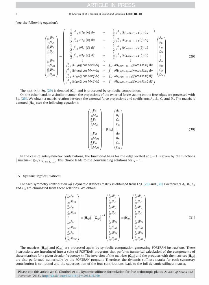
3.5. Dynamic stiffness matrices

For each symmetry contribution αβ a dynamic stiffness matrix is obtained from Eqs. (29) and (30). Coefficients An, Bn, Cnand Dn are eliminated from these relations. We obtain

1αβF01αβMy0

2αβF02αβMx0

⋮1αβFM1αβMxM

2αβFM2αβMyM

0BBBBBBBBBBBBBBBBBBBB@

1CCCCCCCCCCCCCCCCCCCCA

¼ ½Hαβ� � Gαβ

h i�1

1αβW0

1αββx0

2αβW0

2αββy0

⋮1αβWM

1αββxM

2αβWM

2αββyM



¼ ½Kαβ�

1αβW0

1αββx0

2αβW0

2αββy0

⋮1αβWM

1αββxM

2αβWM

2αββyM



(31)

The matrices ½Hαβ� and ½Gαβ� are processed again by symbolic computation generating FORTRAN instructions. Theseinstructions are introduced into a suite of FORTRAN programs that perform numerical calculation of the components ofthese matrices for a given circular frequency ω. The inversion of the matrices ½Gαβ� and the products with the matrices ½Hαβ�are also performed numerically by the FORTRAN program. Therefore, the dynamic stiffness matrix for each symmetrycontribution is computed and the superposition of the four contributions leads to the full dynamic stiffness matrix.







3.6. Harmonic response

The harmonic response of the plate is obtained for any point lying on one of its edges from the superposition of eachsymmetry contribution. For example, the vertical displacement along the right edge (ξ¼ 1) is given as follows:

Wð1;ηÞ ¼ 1SSW0þ

Xþ1

m ¼ 1

1SSWm cosmπηþ

Xþ1

m ¼ 1

1AAWm sin

2m�12

πη

þ1ASW0þ

Xþ1

m ¼ 1

1ASWm cosmπηþ

Xþ1

m ¼ 1

1SAWm sin

2m�12

πη (32)

The first terms of the series not dependent on the geometry variable η give the contribution of the rigid-body modes to theoverall response.

3.7. Modal analysis

Modal analysis is not required because the DSM is not based on a modal superposition. The full systems of Eq. (31) aresolved for each symmetry contribution and for each circular frequency. Nevertheless, a modal analysis can be performed.This analysis deals with a nonlinear eigenvalue problem that is simply based on the computation of determinants of thedynamic stiffness matrices. Sweeping on a given frequency range is done to determine the eigenfrequencies that give a zerodeterminant. Then, the modal displacements are obtained by the resolution of the indeterminate system of equations. Anefficient algorithm was developed by Williams and Wittrick [31] for cases of high modal densities.

4. Numerical examples

To illustrate the application of the method, two numerical examples are presented. The plate considered is made up witha carbon-epoxy orthotropic material defined by its Young's moduli Ex ¼ 18:1� 109 Pa and Ey ¼ 50:9� 109 Pa, its Poisson'sratio νxy ¼ 0:5, its shear modulus Gxy ¼ 11� 109 Pa and its mass density ρ¼ 1526 kg m�3. The 2a� 2b dimensions of theplate are 1 m � 0.5 m, and its thickness is 0.002 mm. Free–free–free–free (FFFF) edge boundary conditions are examined.The DSM responses are compared with those obtained with the FEM (Finite Element Method). The FEM curves presentedare obtained using four-node Discrete Kirchhoff Quadrilateral (DKQ) elements, but with several meshes. The FEM harmonicresponses are obtained without modal truncation to maximize the precision of the results. The full system of linearequations (Eq. (33)) is solved for each circular frequency ω:

½K��ω2½M�� U¼ F (33)

where U is the nodal displacement vector and F is the external nodal force vector.

4.1. Modal analysis

A modal analysis was performed as explained in Section 3.7 for FFFF boundary conditions. This calculation provides thefirst validation of the element developed. Table 2 gives a comparison of the first ten eigenfrequencies processed with thoseobtained with finite element models with DKQ elements (100� 50 elements and 50� 25 elements). Only out-of-planeeigenmodes are considered.

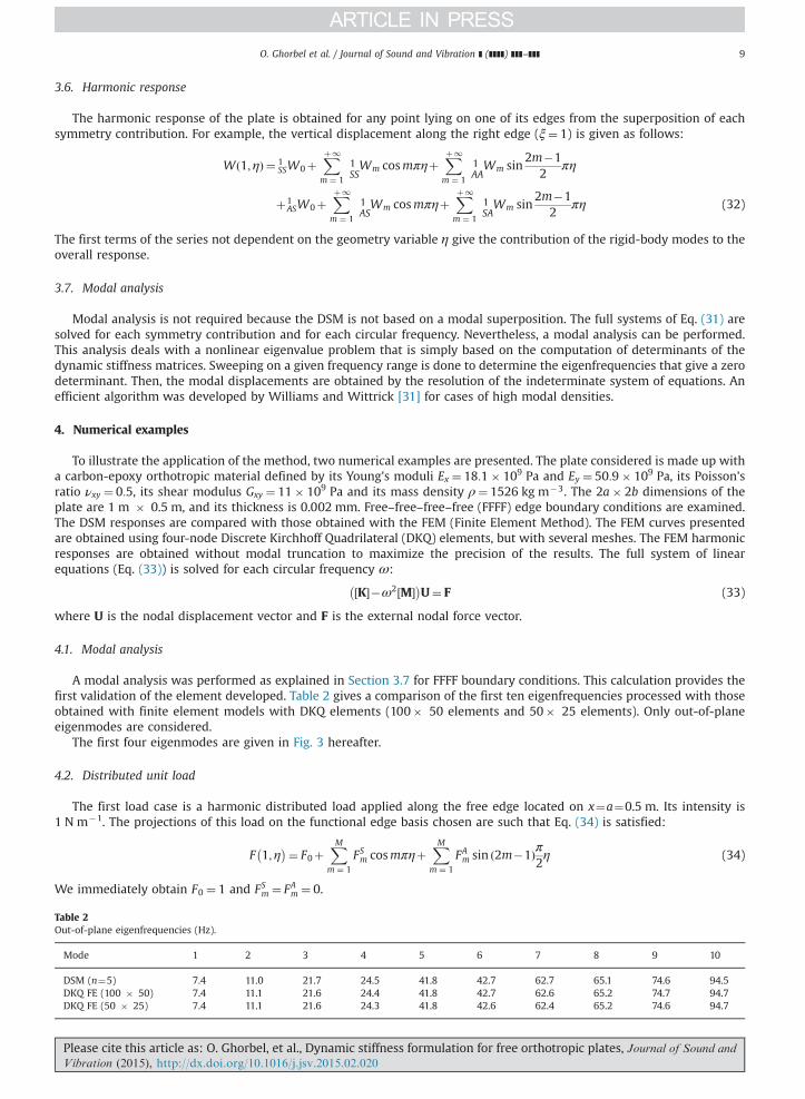
The first four eigenmodes are given in Fig. 3 hereafter.

4.2. Distributed unit load

The first load case is a harmonic distributed load applied along the free edge located on x¼a¼0.5 m. Its intensity is1 N m�1. The projections of this load on the functional edge basis chosen are such that Eq. (34) is satisfied:

F 1;η� �¼ F0þ

XMm ¼ 1

FSm cosmπηþXMm ¼ 1

FAm sin 2m�1ð Þπ2η (34)

We immediately obtain F0 ¼ 1 and FSm ¼ FAm ¼ 0.

Table 2Out-of-plane eigenfrequencies (Hz).

Mode 1 2 3 4 5 6 7 8 9 10

DSM (n¼5) 7.4 11.0 21.7 24.5 41.8 42.7 62.7 65.1 74.6 94.5DKQ FE (100 � 50) 7.4 11.1 21.6 24.4 41.8 42.7 62.6 65.2 74.7 94.7DKQ FE (50 � 25) 7.4 11.1 21.6 24.3 41.8 42.6 62.4 65.2 74.6 94.7






0 20 40 60 80 100 120 140 160 180 200−200

−150

−100

−50

0

50

100

150

frequency (Hz)

20lo

g 10|U

z|

1 DSM (n=5)50 x 25 FEM75 x 35 FEM 100 x 50 FEM

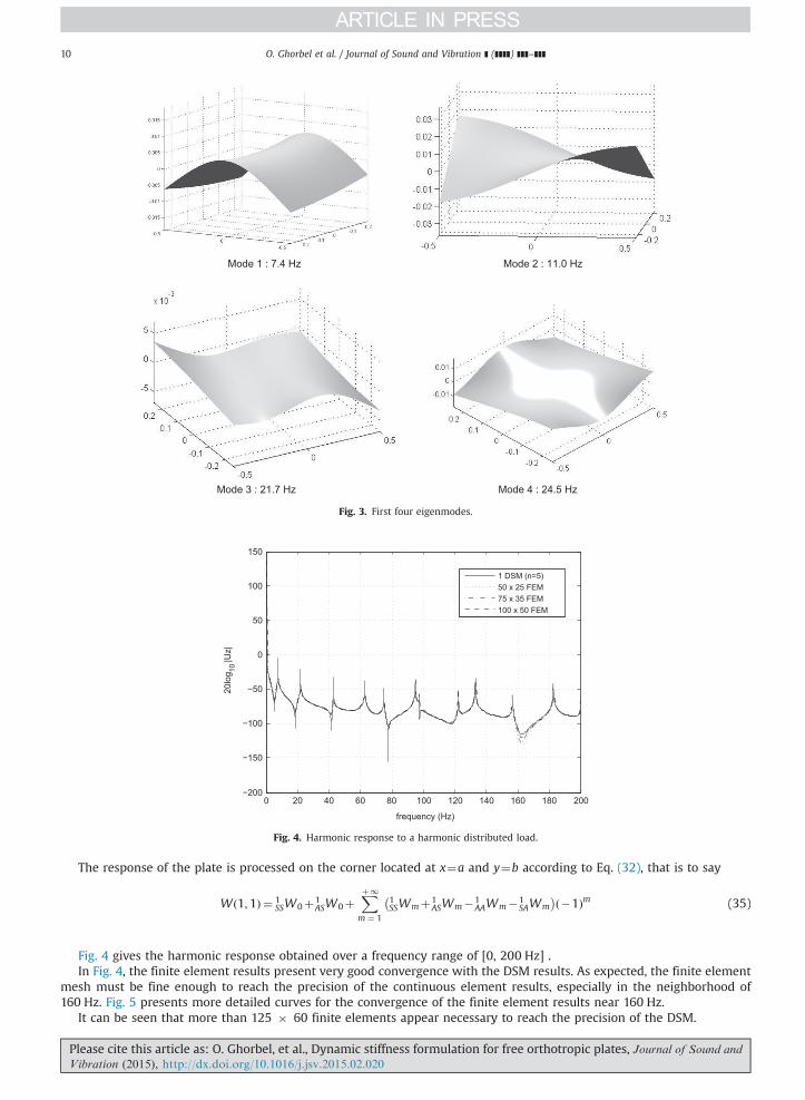
Fig. 4. Harmonic response to a harmonic distributed load.

Mode 1 : 7.4 Hz Mode 2 : 11.0 Hz

Mode 3 : 21.7 Hz Mode 4 : 24.5 Hz

Fig. 3. First four eigenmodes.


The response of the plate is processed on the corner located at x¼a and y¼b according to Eq. (32), that is to say

Wð1;1Þ ¼ 1SSW0þ1

ASW0þXþ1

m ¼ 1

1SSWmþ1

ASWm�1AAWm�1

SAWm� � �1ð Þm (35)

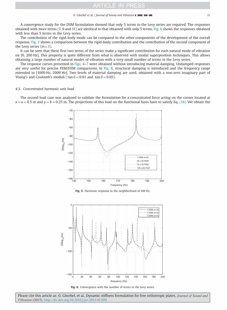
Fig. 4 gives the harmonic response obtained over a frequency range of [0, 200 Hz] .In Fig. 4, the finite element results present very good convergence with the DSM results. As expected, the finite element

mesh must be fine enough to reach the precision of the continuous element results, especially in the neighborhood of160 Hz. Fig. 5 presents more detailed curves for the convergence of the finite element results near 160 Hz.

It can be seen that more than 125 � 60 finite elements appear necessary to reach the precision of the DSM.







A convergence study for the DSM formulation showed that only 5 terms in the Levy series are required. The responsesobtained with more terms (7, 9 and 11) are identical to that obtained with only 5 terms. Fig. 6 shows the responses obtainedwith less than 5 terms in the Levy series.

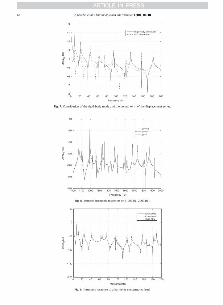
The contribution of the rigid-body mode can be compared to the other components of the development of the overallresponse. Fig. 7 shows a comparison between the rigid-body contribution and the contribution of the second component ofthe Levy series (m¼1).

It can be seen that these first two terms of the series make a significant contribution for each natural mode of vibrationon [0, 200 Hz]. This property is quite different from what is observed with modal superposition techniques. This allowsobtaining a large number of natural modes of vibration with a very small number of terms in the Levy series.

The response curves presented in Figs. 4–7 were obtained without introducing material damping. Undamped responsesare very useful for precise FEM/DSM comparisons. In Fig. 8, structural damping is introduced and the frequency rangeextended to [1000 Hz, 2000 Hz]. Two levels of material damping are used, obtained with a non-zero imaginary part ofYoung's and Coulomb's moduli ( tan δ¼ 0:01 and tan δ¼ 0:05).

4.3. Concentrated harmonic unit load

The second load case was analyzed to validate the formulation for a concentrated force acting on the corner located atx¼ a¼ 0:5 m and y¼ b¼ 0:25 m. The projections of this load on the functional basis have to satisfy Eq. (34). We obtain the

140 150 160 170 180 190 200−180

−160

−140

−120

−100

−80

−60

−40

−20

Frequency (Hz)

20lo

g 10|U

z|

1 DSM (n=5)

50 x 25 FEM

75 x 35 FEM

125 x 60 FEM

Fig. 5. Harmonic response in the neighborhood of 160 Hz.

0 20 40 60 80 100 120 140 160 180 200−150

−100

−50

0

frequency (Hz)

20lo

g 10|U

z|

1 DSM (n=5)1 DSM (n=4)1 DSM (n=2)

Fig. 6. Convergence with the number of terms in the Levy series.






0 20 40 60 80 100 120 140 160 180 200−8

−7

−6

−5

−4

−3

−2

−1

0

frequency (Hz)

20lo

g 10|U

z|

Rigid−body contributionm=1 contribution

Fig. 7. Contribution of the rigid-body mode and the second term of the displacement series.

1000 1100 1200 1300 1400 1500 1600 1700 1800 1900 2000-160

-140

-120

-100

-80

-60

-40

Frequency (Hz)

20lo

g 10|U

z|

tgδ=0.05tgδ=0.01tgδ=0

Fig. 8. Damped harmonic responses on [1000 Hz, 2000 Hz].

0 20 40 60 80 100 120 140 160 180 200−200

−150

−100

−50

0

50

frequency(Hz)

20lo

g 10 |U

z|

1DSM (n=5)100x50 FEM50x25 FEM

Fig. 9. Harmonic response to a harmonic concentrated load.



projections given by the following equation:

F0 ¼12b

FSm ¼ �1ð Þnb

FAm ¼ � �1ð Þnb

8>>>>>>><>>>>>>>:

(36)

The response is processed at the excited point. Fig. 9 gives the responses compared over [0, 200 Hz].Good convergence of the FE results with the DSM response is observed. A convergence study of the DSM results showed

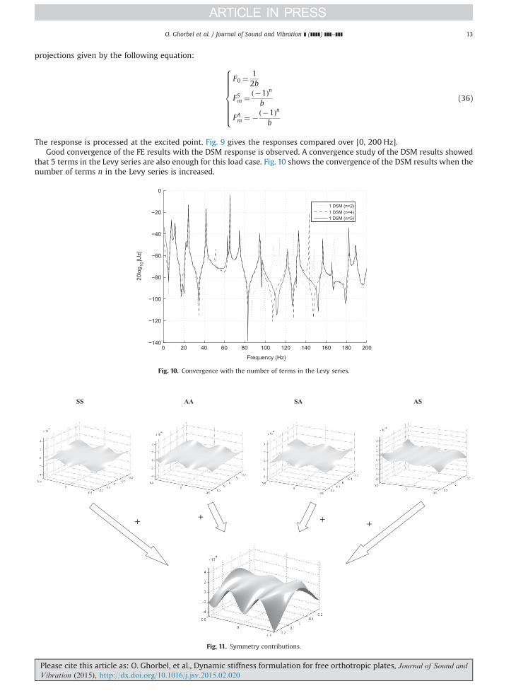
that 5 terms in the Levy series are also enough for this load case. Fig. 10 shows the convergence of the DSM results when thenumber of terms n in the Levy series is increased.

0 20 40 60 80 100 120 140 160 180 200−140

−120

−100

−80

−60

−40

−20

0

Frequency (Hz)

20lo

g 10|U

z|

1 DSM (n=2)1 DSM (n=4)1 DSM (n=5)

Fig. 10. Convergence with the number of terms in the Levy series.

+ + + +

ASAASS AS

Fig. 11. Symmetry contributions.







4.4. Post-processing

Post-processing consists in calculating the displacement and internal force fields in the whole plate. For each symmetrycontribution, once the projections of the edge displacements have been processed, the complex numbers An, Bn, Cn, Dn arecalculated by a numerical inversion of the linear system of Eq. (30). These complex numbers are then used in Eq. (18) toobtain the displacements of any point of the plate and the internal forces are obtained from the force/displacementrelationships (Eq. (9)). In the case of the concentrated load, Fig. 11 shows the four symmetry contributions and the totaldisplacement of the whole plate for a harmonic load of 80 Hz.

5. Conclusion

The dynamic stiffness matrix developed in this paper was used to determine the harmonic response of rectangularorthotropic plates. The method is based on closed-form analytical solutions of the harmonic problem for free edge boundaryconditions. Two load cases were analyzed and the harmonic responses obtained were compared to those obtained by FEMmodels with a commercial FEA software application. Very good convergence of both results was observed for the undampedresponses. The introduction of structural damping was achieved easily with complex elastic moduli. The main advantages ofthe DSM formulation presented are lower memory cost, higher precision and shorter computation time. For example, theprocessing times for 200 frequencies were 41 s and 9 min for DSM (n¼5) and FEM (125 � 60), respectively. The CPUcomputer was an Intel Xeon Quad Core Processor 2.43 GHZ.

References

[1] O.C. Ziekiewicz, R.L. Taylor, The Finite Element Method, fourth edition, Vols. 1 and 2, Mc Graw Hill, London, 1989–91.[2] C.W. Prior Jr, R.M. Barker, A finite-element analysis including transverse shear effects for applications to laminated plates, AIAA Journal 9 (5) (1971)

912–917.[3] R.L. Spilker, A hybrid-stress finite-element formulation for thick multilayer laminates, Computers and Structures 11 (1979) 507–514.[4] C. Jeyachandrabose, J. Kirkhope, Explicit formulation for a high precision triangular laminated anisotropic thin plate finite element, Computers and

Structures 20 (6) (1985) 991–1007.[5] M. di Sciuva, Development of an anisotropic, multilayered shear-deformable rectangular plate element, Computers and Structures 21 (4) (1985)

789–796.[6] N. Grover, B.N. Singh, D.K. Maiti, Analytical and finite element modeling of laminated composite and sandwich plates: an assessment of a new shear

deformation theory for free vibration response, International Journal of Mechanical Sciences 67 (2013) 89–99.[7] H. Nguyen-Xuan, C.H. Thai, T. Nguyen-Thoi, Isogeometric finite element analysis of composite sandwich plates using a higher order shear deformation

theory, Composites: Part B 55 (2013) 558–574.[8] E.L. Albuquerque, P. Sollero, W.S. Venturini, M.H. Aliabadi, Boundary element analysis of anisotropic Kirchhoff plate, International Journal of Sound and

Structures 43 (2006) 4029–4046.[9] T.I. Thinh, M.C. Nuguen, D.G. Ninh, Dynamic stiffness formulation for vibration analysis of thick composite plates resting on non-homogenous

foundations, Composite Structures 108 (2014) 684–695.[10] L. Dozio, Exact vibration solutions for cross-ply laminated plates with two opposite edges simply supported using refined theories of variable order,

Journal of Sound and Vibration 333 (8) (2014) 2347–2359.[11] L. Dozio, Exact free vibration analysis of Lévy FGM plates with higher-order shear and normal deformation theories, Composite Structures 111 (2014)

415–425.[12] H. Thai, S.E. Kim, Levy-type solution for free vibration analysis of orthotropic plates based on two variable refined plate theory, Applied Mathematical

Modeling 36 (2012) 3870–3882.[13] A.W. Leissa, Vibration of Plate, NASA SP-160, Office of Technology Utilization, NASA, Washington DC, 1969.[14] D.J. Gorman, Free Vibration Analysis of Rectangular Plates, Elsevier, Amsterdam, 1982.[15] J.B. Casimir, K. Kevorkian, T. Vinh, The dynamic stiffness matrix of two-dimensional elements: application to Kirchhoff's plate continuous elements,

Journal of Sound and Vibration 287 (2005) 571–589.[16] P.H. Kulla, Continuous elements, some practical examples, ESTEC Workshop Proceedings: Modal Representation of Flexible Structures by Continuum

Methods, 1989.[17] A.Y.T. Leung, Dynamic Stiffness and Substructures, Springer, London, 1993.[18] U. Lee, Spectral Element Method in Structural Dynamics, Wiley, Singapore, 2009.[19] J.B. Casimir, C. Duforet, T. Vinh, Dynamic behaviour of structures in large frequency range by continuous element methods, Journal of Sound and

Vibration 267 (2003) 1085–1106.[20] J.R. Banerjee, H. Su, D.R. Jackson, Free vibration of rotating tapered beams using the dynamic stiffness method, Journal of Sound and Vibration 298 (4–5)

(2006) 1034–1054.[21] J.R. Banerjee, W.D. Gunawardana, Dynamic stiffness matrix development and free vibration analysis of a moving beam, Journal of Sound and Vibration

303 (1–2) (2007) 135–143.[22] D. Tounsi, J.B. Casimir, M. Haddar, Dynamic stiffness formulation for circular rings, Computers and Structures 112–113 (2012) 258–265.[23] M. Boscolo, J.R. Banerjee, Layer-wise dynamic stiffness solution for free vibration analysis of laminated composite plates, Journal of Sound and Vibration

333 (1) (2014) 200–227.[24] J.B. Casimir, M.C. Nguyen, I. Tawfiq, Thick shells of revolution: derivation of the dynamic stiffness matrix of continuous elements and application to a

tested cylinder, Computers and Structures 85 (2007) 1845–1857.[25] D. Tounsi, J.B. Casimir, S. Abid, I. Tawfiq, M. Haddar, Dynamic stiffness formulation and response analysis of stiffened shells, Computers and Structures

132 (2014) 75–83.[26] F. Fazzolari, A refined dynamic stiffness element for free vibration analysis of cross-ply laminated composite cylindrical and spherical shallow shells,

Composites Part B: Engineering 62 (2014) 143–158.[27] B.A. Akesson, PFVIBAT – a computer program for plane frame vibration analysis by an exact method, International Journal for Numerical Methods in

Engineering 10 (1976) 1221–1231.[28] C. Duforet, Dynamic study of an assembling of rods in medium and higher frequency ranges – computer code ETAPE, Third Colloquium on New Trends

in Structure Calculations-Bastia, Corsica-Proceedings, 1985, pp. 229–246 (in French).



http://refhub.elsevier.com/S0022-460X(15)00154-6/sbref202
















































[29] M.S. Anderson, F.W. Williams, J.R. Banerjee, B.J. Durling, C.L. Herstorm, D. Kennedy, D.B. Warnaar, User manual for BUNVIS-RG: an exact buckling andvibration program for lattice structures, with repetitive geometry and substructuring options, NASA Technical Memorandum 87669, 1986.

[30] F.W. Williams, D. Kennedy, R. Butler, M.S. Anderson, VICONOPT: program for exact vibration and buckling analysis or design of prismatic plateassemblies, AIAA Journal 29 (1991) 1927–1928.

[31] F.W. Williams, W.H. Wittrick, An automatic computational procedure for calculating natural frequencies of skeletal structures, International Journal ofMechanical Sciences 12 (9) (1970) 781–791.










Documents

1-s2.0-S0022460X15001546-main