arX

iv:1

711.

0860

6v2

[cs

.IT

] 2

9 N

ov 2

017

1

Robust Beamforming for Physical Layer

Security in BDMA Massive MIMO

Fengchao Zhu, Feifei Gao, Hai Lin, Shi Jin, and Junhui Zhao

Abstract

In this paper, we design robust beamforming to guarantee the physical layer security for a multiuser

beam division multiple access (BDMA) massive multiple-input multiple-output (MIMO) system, when

the channel estimation errors are taken into consideration. With the aid of artificial noise (AN), the pro-

posed design are formulated as minimizing the transmit power of the base station (BS), while providing

legal users and the eavesdropper (Eve) with different signal-to-interference-plus-noise ratio (SINR). It

is strictly proved that, under BDMA massive MIMO scheme, the initial non-convex optimization can be

equivalently converted to a convex semi-definite programming (SDP) problem and the optimal rank-one

beamforming solutions can be guaranteed. In stead of directly resorting to the convex tool, we make

one step further by deriving the optimal beamforming direction and the optimal beamforming power

allocation in closed-form, which greatly reduces the computational complexity and makes the proposed

design practical for real world applications. Simulation results are then provided to verify the efficiency

of the proposed algorithm.

Index Terms

Robust beamforming, massive MIMO, physical layer security, beam division multiple access (BDMA),

closed-form.

F. Zhu is with High-Tech Institute of Xi’an, Xi’an, Shaanxi 710025, China (e-mail: fengchao zhu@126.com). F. Gao is

with the State Key Laboratory of Intelligent Technology and Systems, Tsinghua National Laboratory for Information Science

and Technology, Department of Automation, Tsinghua University, Beijing, 100084, China (e-mail: feifeigao@ieee.org). H.

Lin is with the Department of Electrical and Information Systems, Osaka Prefecture University, Sakai, Osaka, Japan (e-mail:

hai.lin@ieee.org). S. Jin is with the National Communications Research Laboratory, Southeast University, Nanjing 210096, P. R.

China (email: jinshi@seu.edu.cn). J. Zhao is with School of Information Engineering, East China Jiaotong University, Nanchang,

330013, China, and is also with School of Electronic and Information Engineering, Beijing Jiaotong University, Beijing, 100044,

China (email: eeejhzhao@163.com).

2

I. INTRODUCTION

Massive multiple-input multiple-output (MIMO) [1] is one of the key technologies for 5G

wireless communications [2], which utilizes a very large number of antennas at the base station

(BS) to provide low power consumption, high spectral efficiency, security, and reliable linkage. It

was shown in [3] that the propagation channel vectors of different users become asymptotically

orthogonal, where the effects of uncorrelated noise and intra-cell interference will be eliminated

when the number of antennas at the BS grows to infinity. As a result, simple linear signal

processing approaches, i.e., matched filter (MF) and zero-forcing beamforming can be used in

massive MIMO systems [4]. However, a prerequisite of enjoying above benefits is the availability

of channel state information (CSI). There are three main approaches of low-complex channel

estimation algorithms that referred to different expansion basis to represent the sparsity inside

channels [5]–[11]. For example, the authors in [5], [6] applied a low-rank approximation of the

channel covariance matrix to reduce the effective channel parameters of massive MIMO. The

authors in [7]–[9] proposed an angle division multiple access (ADMA) model and the massive

MIMO channels could be represented by a few channel gain and angular parameters. Moreover,

[10], [11] designed a beam division multiple access (BDMA) scheme and a few orthogonal basis

from discrete Fourier transform (DFT) are used to approximate the channel vectors. Nevertheless,

perfect CSI are not available in practice due to: (i) all [5]–[11] are based on approximately-sparse

model and there must be residue errors; (ii) additive noise always exist at the receiver. Therefore,

the channel estimation errors should be taken into consideration in the subsequent transmission

design.

On the other side, secrecy and privacy are also critical concerns for 5G communication

systems, where the physical layer security has drawn considerable interest since it can pre-

vent eavesdropping without upper layer data encryption. The information-theoretic approach to

guarantee secrecy was initiated by Wyner [12], where it was shown that confidential messages

transmission could be achieved by exploiting the physical characteristics of the wireless channel.

Then the results of [12] was generalized to different channel models, i.e., the broadcast channels

[13], the single-input single-output (SISO) fading channels [14], the multiple access channels

(MAC) [15], and the multiple-input multiple-output (MIMO) channels [16]. The authors of [17]

3

first investigated the limiting physical layer security performance when the number of antennas

approaches infinity in massive MIMO systems, and then [18], [19] studied the physical layer

security in massive MIMO relay channel and massive MIMO Rician Channel, respectively.

The authors of [20]–[22] considered the asymptotic achievable secrecy rate in massive MIMO

systems, where it was shown that under certain orthogonality conditions, the secrecy rate loss

introduced by the eavesdropper could be completely mitigated. However, all [17]–[22] do not take

channel estimation errors into consideration. To the best of the authors’ knowledge, the optimal

solution of robust beamforming for the physical layer security of massive MIMO systems has

not been reported yet.

In this paper, we consider robust beamforming for the physical layer security of multiuser mas-

sive MIMO systems following BMDA scheme [10], [11], where the estimated channels are lied

orthogonally to each other and the channel estimation errors are bounded by ball constants. The

proposed design utilizes simultaneous robust information and artificial noise (AN) beamforming

to provide the legal users and Eve with different signal-to-interference-and-noise ratio (SINR),

meanwhile minimizing the transmit power of BS. The resulted problem is a well-known NP-

hard [23] optimization, where the computational complexity [24] increases exponentially with

the number of antennas. Consequently, existing robust beamforming algorithms for conventional

communication systems [25]–[28] cannot be applied in massive MIMO systems due to their

forbiddingly huge computational complexity. Nevertheless, we demonstrate that under the BDMA

massive MIMO scheme, the proposed design can be globally solved. More importantly, the

optimal robust beamforming vectors can be derived in closed-form, which will greatly reduce

the computational complexity and is suitable for practical applications. Interestingly, it is shown

that the AN beamforming is not necessary for the proposed robust optimization.

The rest of this paper is organized as follows: Section II describes the BDMA massive MIMO

channel model and formulates the proposed robust design; Section III converts the initial non-

convex optimization into a convex semi-definite programming (SDP) and proves the optimality

of semi-definite relaxation (SDR); Closed-form solutions for the power allocation problem are

derived in Section IV; Simulation results are provided in Section V and conclusions are drawn

in Section VI.

4

Notation: Vectors and matrices are boldface small and capital letters, respectively; The Her-

mitian, inverse and Moore-Penrose inverse of A are denoted by AH, A−1 and A† respectively;

Tr(A) defines the trace; I and 0 represent an identity matrix and an all-zero matrix, respectively,

with appropriate dimensions; A � 0 and A ≻ 0 mean that A is positive semi-definite and

positive definite, respectively; The distribution of a circularly symmetric complex Gaussian

(CSCG) random variable with zero mean and variance σ2 is defined as CN (0, σ2), and ∼ means

“distributed as”; Ra×b and Ca×b denote the spaces of a×b matrices with real- and complex-valued

entries, respectively; ‖x‖ is the Euclidean norm of a vector x.

II. SYSTEM MODEL AND PROBLEM FORMULATION

A. System Model

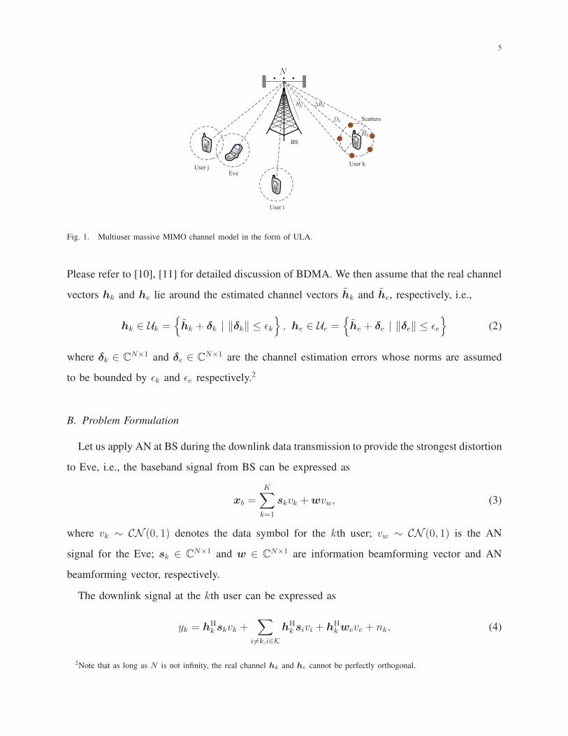
Let us consider physical layer security for a multiuser massive MIMO system shown in Fig. 1.

It is assumed that the BS is equipped with N ≫ 1 antennas in the form of uniform linear array

(ULA), where the antenna spacing is less than or equal to half wavelength. There are K legal

users and one Eve randomly distributed in the coverage area, where all the legal users and the

Eve are quipped with single antenna. The channel from the kth user to BS can be expressed as

[5], [9] hk =∫

θ∈Θkαk(θ)a(θ)dθ, where Θk is the incoming angular spread of user-k and αk(θ)

is the corresponding spatial power spectrum. Moreover, a(θ) ∈ CN×1 is the steering vector that

can be expressed as a(θ) =[

1, ej2πdλ

sin θ, . . . , ej2πdλ

(N−1) sin θ]H

, where d is the antenna spacing

and λ denotes the signal wavelength. Similarly, the channel from the Eve to BS can be expressed

as he =∫

θ∈Θeαe(θ)a(θ)dθ, where Θe is the incoming angular spread of Eve and αe(θ) is the

corresponding spatial power spectrum.

In this paper, we adopt the recently popular low complexity BDMA channel estimation scheme

[10], [11] such that pilots of different users are transmitted through orthogonal spatial directions1,

and the estimated channels for different users must be orthogonal, i.e.,

hHi hj = 0, hH

i he = 0, ∀i 6= j, (1)

1In particular, the columns of discrete Fourier transform (DFT) matrix with non-overlap indices are assigned to different users

as the training directions. Such a scheme is not optimal in terms of training design but could be implemented with much higher

efficiency. Moreover, as long as N is large, which is the case of massive MIMO, the performance loss of BDMA channel

estimation is small compared to the optimal one.

5

: : :N

¢ kk

Dk

Rk

Fig. 1. Multiuser massive MIMO channel model in the form of ULA.

Please refer to [10], [11] for detailed discussion of BDMA. We then assume that the real channel

vectors hk and he lie around the estimated channel vectors hk and he, respectively, i.e.,

hk ∈ Uk ={

hk + δk | ‖δk‖ ≤ ǫk

}

, he ∈ Ue ={

he + δe | ‖δe‖ ≤ ǫe

}

(2)

where δk ∈ CN×1 and δe ∈ C

N×1 are the channel estimation errors whose norms are assumed

to be bounded by ǫk and ǫe respectively.2

B. Problem Formulation

Let us apply AN at BS during the downlink data transmission to provide the strongest distortion

to Eve, i.e., the baseband signal from BS can be expressed as

xb =K∑

k=1

skvk +wvw, (3)

where vk ∼ CN (0, 1) denotes the data symbol for the kth user; vw ∼ CN (0, 1) is the AN

signal for the Eve; sk ∈ CN×1 and w ∈ CN×1 are information beamforming vector and AN

beamforming vector, respectively.

The downlink signal at the kth user can be expressed as

yk = hHk skvk +

∑

i 6=k,i∈K

hHk sivi + hH

kweve + nk, (4)

2Note that as long as N is not infinity, the real channel hk and he cannot be perfectly orthogonal.

6

where nk ∼ CN (0, σ2k) represents the antenna noise of the kth user. The downlink signal at the

Eve can be expressed as

ye =K∑

k=1

hHe skvk + hH

e weve + ne, (5)

where nk ∼ CN (0, σ2k) represents the antenna noise of the Eve. Then the secret rate for the kth

user are expressed as

Rk = log2

1+‖hH

k sk‖2

∑

i 6=k

‖hHk si‖

2+‖hHkwe‖

2+σ2k

−log2

1+‖hH

e sk‖2

∑

i 6=k

‖hHe si‖

2+‖hHe we‖

2+σ2e

≥ log2 (1 + γk)− log2 (1 + γe,k) , (6)

where γk is the receive SINR for the kth user, and γe,k is the receive SINR for Eve when Eve

aims to eavesdrop the kth user. Note that when γk > γe,k > 0, ∀k ∈ {1, . . . , K}, we could

always obtain non-zero secret rate for each users, which implies that the physical layer security

could be strictly guaranteed.

Our target is to design simultaneous information beamforming vectors {sk} and AN beam-

forming vector we to provide legal users and the Eve with different SINRs, meanwhile mini-

mizing the transmit power of BS. Taking the channel estimation errors into consideration, the

robust transmit beamforming design can be formulated as

P1 : min{sk},we

‖we‖2 +

K∑

k=1

‖sk‖2 (7)

s.t.‖hH

e sk‖2

∑

i 6=k

‖hHe si‖

2 + ‖hHe we‖

2 + σ2e

≤ γe,k, he ∈ Ue, (8)

‖hHk sk‖

2

∑

i 6=k

‖hHk si‖

2 + ‖hHkwe‖

2 + σ2k

≥ γk, ∀hk ∈ Uk, (9)

k = 1, 2, . . . , K, (10)

where γe,k > 0 is the maximum allowable SINR for Eve, and γk > 0 is the desired SINR for the

kth user. Note that the optimal solutions of P1 are very hard to obtain in conventional MIMO

7

systems3. Nevertheless, we will next show that P1 could be globally solved utilizing property

(1) of BDMA massive MIMO systems.

III. OPTIMAL ROBUST BEAMFORMING

A. Problem Reformulation

The main difficulty of solving P1 lies in the constraints (8) and (9). Substituting (2) into (8),

we can equivalently rewrite (8) as

(

he+δe

)H(

∑

i 6=k

sisHi +wew

He −

1

γe,ksks

Hk

)

(

he+δe

)

+σ2e ≥ 0,

−δHe Iδe + ǫ2e ≥ 0, k = 1, 2, . . . , K.

(11)

Substituting (2) into (9), we can equivalently rewrite (9) as

(

hk+δk

)H(

1

γksks

Hk −∑

i 6=k

sisHi −wew

He

)

(

hk+δk

)

−σ2k ≥ 0,

−δHk Iδk + ǫ2k ≥ 0, k = 1, 2, . . . , K.

(12)

According to the Lemma of S-Procedure [29], we know that the constraints in (11) hold true

if and only if there exists µe,k ≥ 0, k = 1, 2, . . . , K such that

Xe,k + µe,kI Xe,khe

hHe X

He,k hH

e Xe,khe + σ2e − µe,kǫ

2e

� 0, (13)

where for simplicity, we define Xe,k as

Xe,k =∑

i 6=k

sisHi +wew

He −

1

γe,ksks

Hk . (14)

Meanwhile, the constraints in (12) hold true if and only if there exists µs,k ≥ 0, k = 1, 2, . . . , K

such that

Xs,k + µs,kI Xs,khk

hHkX

Hs,k hH

kXs,khk − σ2k − µs,kǫ

2k

� 0, (15)

where for simplicity, we define Xs,k as

Xs,k =1

γksks

Hk −∑

i 6=k

sisHi −wew

He . (16)

3The proposed design P1 has been proven to be NP hard in conventional communication systems [27], where it is very

difficult to obtain the optimal beamforming vectors.

8

It is then clear that P1 can be equivalently re-expressed as

P1−EQV : min{µe,k},{µs,k},we,{sk}

Tr(We) +

K∑

k=1

Tr(Sk) (17)

s.t.

Xe,k + µe,kI Xe,khe

hHe X

He,k hH

e Xe,khe + σ2e − µe,kǫ

2e

� 0, (18)

Xs,k + µs,kI Xs,khk

hHkX

Hs,k hH

kXs,khk − σ2k − µs,kǫ

2k

� 0, (19)

Xe,k =∑

i 6=k

Si +We −1

γe,kSk, (20)

Xs,k =1

γkSk −

∑

i 6=k

Si −We, (21)

µe,k ≥ 0, µs,k ≥ 0, (22)

We = wewHe , Sk = sks

Hk , k = 1, 2, . . . , K, (23)

where {µe,k} and {µs,k} are the auxiliary variables generated by the S-Procedure. Note that the

nonlinear constraints in (23) are equivalent to:

We � 0, Sk � 0, Rank(We) = 1, Rank(Sk) = 1. (24)

However, P1−EQV is still very hard to solve since the rank constraint in (23) is non-convex.

Dropping the the rank constraints Rank(We) = 1 and Rank(Sk) = 1 (the SDR technique [30]),

we can obtain the following relaxed convex optimization:

P1−SDR : min{µe,k},{µs,k},We,{Sk}

Tr(We) +

K∑

k=1

Tr(Sk) (25)

s.t. (18) ∼ (22), (26)

We � 0, Sk � 0, k = 1, 2, . . . , K, (27)

which is a semi-definite programming (SDP) problem that can be efficiently solved by the

standard convex optimization tools [23]. However, the SDR technique does not guarantee rank-

one solutions for the relaxed optimization. Nevertheless, we will next show that P1−SDR

indeed guarantees rank-one solutions for BDMA massive MIMO systems, i.e., P1−SDR is

equivalent to P1−EQV.

9

B. Optimal Rank-one Solutions

The following propositions will be useful throughout the rest of the paper.

Proposition 1: Suppose {µ⋆e,k} and {µ⋆

s,k} are the optimal auxiliary variables of P1−SDR.

There must be

(a) µ⋆e,k > 0, ∀k ∈ {1, . . . , K}; (b) µ⋆

s,k > 0, ∀k ∈ {1, . . . , K}.

Proof: See Appendix A.

Proposition 2: Suppose W ⋆e and {S⋆

k} are the optimal transmit covariances of P1−SDR.

There must be

(a) Rank(

X⋆e,k + µ⋆

e,kI)

≥ 1, ∀k ∈ {1, . . . , K}; (b) Rank(

X⋆s,k + µ⋆

s,kI)

≥ 1, ∀k ∈ {1, . . . , K}.

Proof: See Appendix B.

Remark 1: Proposition 1 and Proposition 2 indicate that the optimal AN and information

transmit covariance could not be full-rank, i.e., Rank (W ⋆e ) < N and Rank (S⋆

k) < N, ∀k ∈

{1, . . . , K}. Moreover, from (B.8) in Appendix B, we know that Rank (W ⋆e ) and Rank (S⋆

k)

can be further constrained as Rank (W ⋆e ) ≤ K + 1 and Rank (S⋆

k) ≤ K + 1, ∀k ∈ {1, . . . , K}.

From Proposition 1 and Proposition 2, we can reformulate P1−SDR to gain more insightful

solutions. Let the eigenvalue decomposition (EVD) of Xe,k be Xe,k = Ue,kΛe,kUHe,k with the

eigenvalues qe,k,1 ≥ . . . ≥ qe,k,N , and the EVD of Xs,k be Xs,k = Us,kΛs,kUHs,k with the

eigenvalues qs,k,1 ≥ . . . ≥ qs,k,N . Due to the fact that µe,kI = Ue,k (µe,kI)UHe,k and µs,kI =

Us,k (µs,kI)UHs,k, the EVDs of Xe,k + µe,kI and Xs,k + µs,kI can be represented as

Xe,k + µe,kI = Ue,k (Λe,k + µe,kI)UHe,k, Xs,k + µs,kI = Us,k (Λs,k + µs,kI)U

Hs,k, (28)

respectively, where Λe,k+µe,kI is diagonal with the eigenvalues qe,k,1+µe,k ≥ . . . ≥ qe,k,N+µe,k

and Λs,k + µs,kI is diagonal with the eigenvalues qs,k,1 + µs,k ≥ . . . ≥ qs,k,N + µs,k. Using

Proposition 1 and Proposition 2, it is easily known that qe,k,1 + µe,k > 0 and qs,k,1 + µs,k > 0

hold. Then assuming Rank (Xe,k + µe,kI) = le,k ≥ 1 and Rank (Xs,k + µs,kI) = ls,k ≥ 1, there

are

qe,k,i + µe,k = 0, ∀i ∈ {le,k + 1, . . . , N}, ∀k ∈ {1, . . . , K}, (29)

qs,k,i + µs,k = 0, ∀i ∈ {ls,k + 1, . . . , N}, ∀k ∈ {1, . . . , K}. (30)

10

Define Σe,k,+ and Σs,k,+ as

Σe,k,+ =

qe,k,1 + µe,k 0 0

0. . . 0

0 0 qe,k,le,k + µe,k

,Σs,k,+ =

qs,k,1 + µs,k 0 0

0. . . 0

0 0 qs,k,le,k + µs,k

,

respectively. The Moore-Penrose inverses [31] of Xe,k + µe,kI and Xs,k + µs,kI can be derived

as4

(Xe,k + µe,kI)† = Ue,k

Σ−1e,k,+ 0

0 0

UHe,k, (Xs,k + µs,kI)

† = Us,k

Σ−1s,k,+ 0

0 0

UHs,k, (31)

respectively. Then we provide the following lemma.

Lemma 2 (Generalized Schur’s Complement [32]): Let M =[

A,B;BH,C]

be a Hermitian

matrix. Then, M � 0 if and only if C − BHA†B � 0 and(

I −AA†)

B = 0 (assuming

A � 0), or A−BC†BH � 0 and(

I −CC†)

BH = 0 (assuming C � 0), where A† and C†

are the generalized inverses of A and C, respectively.

Using Lemma 2, we know that P1−SDR could be equivalently rewritten as

P1−SDR−EQV :

min{µe,k},{µs,k},We,{Sk}

Tr(We) +K∑

k=1

Tr(Sk) (32)

s.t. Xe,k + µe,kI � 0, Xs,k + µs,kI � 0, (33)[

I − (Xe,k + µe,kI) (Xe,k + µe,kI)†]

Xe,khe = 0, (34)

hHe Xe,khe + σ2

e − µe,kǫ2e − hH

e XHe,k (Xe,k + µe,kI)

†Xe,khe ≥ 0, (35)

[

I − (Xs,k + µs,kI) (Xs,k + µs,kI)†]

Xs,khk = 0, (36)

hHkXs,khk − σ2

k − µs,kǫ2k − hH

kXHs,k (Xs,k + µs,kI)

†Xs,khk ≥ 0, (37)

Xe,k =∑

i 6=k

Si +We −1

γe,kSk, (38)

Xs,k =1

γkSk −

∑

i 6=k

Si −We, (39)

µe,k ≥ 0, µs,k ≥ 0, We � 0, Sk � 0, k = 1, 2, . . . , K, (40)

4Note that if Rank (Xe,k + µe,kI) = N and Rank (Xs,k + µs,kI) = N , then there are (Xe,k + µe,kI)† =

(Xe,k + µe,kI)−1

and (Xs,k + µs,kI)† = (Xs,k + µs,kI)

−1.

11

where the constraints in (33)∼(37) are derived from (18) and (19).

Next, we will investigate the constraints (33)∼(37) to obtain more insightful solutions. Due

to the fact that

(Xe,k + µe,kI) (Xe,k + µe,kI)† = Ue,k

I le,k×le,k 0

0 0(N−le,k)×(N−le,k)

UHe,k,

Eq. (34) can be expressed as

[

I − (Xe,k + µe,kI) (Xe,k + µe,kI)†]

Xe,khe

=Ue,k

0le,k×le,k 0

0 I(N−le,k)×(N−le,k)

UHe,kUe,k

Λle,k×le,ke,k 0

0 Λ(N−le,k)×(N−le,k)

e,k

UHe,khe

=Ue,k

0 0

0 Λ(N−le,k)×(N−le,k)

e,k

UHe,khe = 0, (41)

which says that Λ(N−le,k)×(N−le,k)

e,k

[

uHe,k,le,k+1, . . . ,u

He,k,N

]

he = 0 holds true, where ue,k,i is the

ith column of Ue,k. Similarly, Eq. (36) can be expressed as

[

I − (Xs,k + µs,kI) (Xs,k + µs,kI)†]

Xs,khk

=Us,k

0ls,k×ls,k 0

0 I(N−ls,k)×(N−ls,k)

UHs,kUs,k

Λls,k×ls,ks,k 0

0 Λ(N−ls,k)×(N−ls,k)

s,k

UHs,khk

=Us,k

0 0

0 Λ(N−ls,k)×(N−ls,k)s,k

UHs,khk = 0, (42)

which implies that Λ(N−ls,k)×(N−ls,k)

s,k

[

uHs,k,ls,k+1, . . . ,u

Hs,k,N

]

hk = 0 holds true, where us,k,i is

the ith column of Us,k.

Due to Xe,k = XHe,k, Eq. (35) can be expressed as

hHe Xe,khe + σ2

e − µe,kǫ2e − hH

e XHe,k (Xe,k + µe,kI)

†Xe,khe

=Tr(

HeXe,k

)

+ σ2e − µe,kǫ

2e − Tr

[

HeXHe,k (Xe,k + µe,kI)

†Xe,k

]

=Tr{(

HeXe,k

) [

I − (Xe,k + µe,kI)†Xe,k

]}

+ σ2e − µe,kǫ

2e ≥ 0, (43)

12

where He = hehHe . Similarly, Eq. (37) can be expressed as

hHkXs,khk − σ2

k − µs,kǫ2k − hH

kXHs,k (Xs,k + µs,kI)

†Xs,khk

=Tr(

HkXs,k

)

− σ2k − µs,kǫ

2k − Tr

[

HkXHs,k (Xs,k + µs,kI)

†Xs,k

]

=Tr{(

HkXs,k

) [

I − (Xs,k + µs,kI)†Xs,k

]}

− σ2k − µs,kǫ

2k ≥ 0, (44)

where Hk = hkhHk .

Theorem 1: When Eq. (1) holds, the optimal solutions of P1−SDR−EQV must satisfy

(a) Rank (W ⋆e ) ≤ 1, where W ⋆

e = w⋆ew

⋆He = P ⋆

e hehHe /‖he‖

2 is the optimal AN transmit

covariance that can be derived through the closed-form AN beamforming vector, and P ⋆e

is the power allocated for the AN beamforming;

(b) Rank (S⋆k) ≤ 1, ∀k ∈ {1, . . . , K}, where S⋆

k = s⋆ks⋆Hk = P ⋆

k hkhHk /‖hk‖2 is the optimal

information transmit covariance that can be derived through the closed-form information

beamforming vectors, and P ⋆k is the power allocated for the kth information beamforming.

Proof: See Appendix C.

Remark 2: Theorem 1 indicates that simultaneous AN- and information-beamforming is the

optimal transmit strategy for P1−SDR−EQV rather than the joint precoding scheme. Thus,

the SDR solutions are indeed optimal for P1.

IV. OPTIMAL POWER ALLOCATION

In Section III, it is shown that the optimal solutions of P1 could be derived by solv-

ing P1−SDR−EQV, where the optimal beamforming vectors are derived in closed-form.

However, the optimal power allocations P ⋆e and {P ⋆

k } remain unknown. Since the optimal

AN-beamforming and information-beamforming vectors are w⋆e =

√

P ⋆e he/‖he‖ and s⋆k =

√

P ⋆k hk/‖hk‖, P1 can be simplified to

P2 : min{µe,k},{µs,k},Pe,{Pk}

Pe +

K∑

k=1

Pk (45)

s.t.µe,kPe‖he‖2

µe,k + Pe

+ σ2e − µe,kǫ

2e ≥ 0, (46)

µs,kPk‖hk‖2

µs,kγk + Pk

− σ2k − µs,kǫ

2k ≥ 0, (47)

µe,k > 0, µs,k > 0, Pe ≥ 0, Pk ≥ 0, k = 1, 2, . . . , K. (48)

13

Define

fe,k(µe,k, Pe) ,µe,kPe‖he‖

2

µe,k + Pe

, fs,k(µs,k, Pk) ,µs,kPk‖hk‖

2

µs,kγk + pk, (49)

whose Hessian matrixes are given by

∇2fe,k(µe,k, Pe) =−2‖he‖2

(µe,k + Pe)3

P 2e −µe,kPe

−µe,kPe µ2e,k

� 0, (50)

∇2fs,k(µs,k, Pk) =−2γk‖hk‖2

(µs,kγk + Pk)3

P 2k −µs,kPk

−µs,kPk µ2s,k

� 0, (51)

respectively, which implies that fe,k(µe,k, Pe) and fs,k(µs,k, Pk) are concave functions. Thus, P2

is a convex optimization.

A. Optimal AN Power Allocation

The optimal AN power allocation P ⋆e can be summarized in the following theorem.

Theorem 2: At the optimal point, the AN power allocation P ⋆e of P2 must satisfy

P ⋆e = 0, (52)

where the corresponding auxiliary variables {µe,k} satisfy µe,k = σ2e/ǫ

2e > 0, ∀k ∈ {1, . . . , K}.

Proof: Let us show that P ⋆e = 0 from contradiction. Assume {µ⋆

e,k}, {µ⋆s,k}, P ⋆

e and {P ⋆k }

are the optimal solutions of P2, where P ⋆e > 0 is satisfied. Then we can provide a group of

new solutions:

µ∗e,k =

σ2e

ǫ2e, µ∗

s,k = µ⋆s,k, P ∗

e = 0, P ∗k = P ⋆

k , ∀k ∈ {1, . . . , K}. (53)

Substituting {µ∗e,k}, {µ∗

s,k}, P ∗e and {P ∗

k } into P2, we obtain

P ∗e +

K∑

k=1

P ∗k = 0 +

K∑

k=1

P ⋆k < P ⋆

e +K∑

k=1

P ⋆k (54)

µ∗e,kP

∗e ‖he‖2

µ∗e,k + P ∗

e

+ σ2e − µ∗

e,kǫ2e = 0, (55)

µ∗s,kP

∗k ‖hk‖2

µ∗s,kγk + P ∗

k

− σ2k − µ∗

s,kǫ2k ≥ 0, (56)

µ∗e,k =

σ2e

ǫ2e> 0, µ∗

s,k = µ⋆s,k > 0, P ∗

e = 0, P ∗k = P ⋆

k ≥ 0, k = 1, 2, . . . , K. (57)

14

From (55)∼(57), we conclude that {µ∗e,k}, {µ∗

s,k}, P ∗e and {P ∗

k } satisfy all the constraints of

P2. While we know from (55) that {µ∗e,k}, {µ∗

s,k}, P ∗e and {P ∗

k } will always provide smaller

object value, which contradicts the assumption that {µ⋆e,k}, {µ⋆

s,k}, P ⋆e and {P ⋆

k } are the optimal

solutions. Thus, at the optimal point there must be P ⋆e = 0.

Theorem 2 says that in order to optimally guarantee the the physical layer security for BDMA

massive MIMO system, one should not adopt the AN beamforming, which is much different

from the conventional MIMO case.

B. Optimal Information Power Allocation

The Lagrange of P2 is defined as

L ({µe,k}, {µs,k}, Pe, {Pk}, {k}, {ξk}) = Pe +

K∑

k=1

Pk

−K∑

k=1

[

k

(

µe,kPe‖he‖2

µe,k + Pe

+ σ2e − µe,kǫ

2e

)]

−K∑

k=1

[

ξk

(

µs,kPk‖hk‖2

µs,kγk + Pk

− σ2k − µs,kǫ

2k

)]

, (58)

where {k ≥ 0} and {ξk ≥ 0} are the dual variables associated with the constraints (46) and

(47), respectively. The Karush-Kuhn-Tucker (KKT) conditions related to {µe,k} {µs,k}, Pe and

{Pk} can be formulated as ∀k ∈ {1, . . . , K}

∂L

∂µ⋆e,k

= ⋆kǫ

2e −

⋆kP

⋆2e ‖he‖2

(µ⋆e,k + P ⋆

e )2= 0, (59)

∂L

∂µ⋆s,k

= ξ⋆kǫ2k −

ξ⋆kP⋆2k ‖hk‖2

(µ⋆s,kγk + P ⋆

k )2= 0, (60)

∂L

∂P ⋆e

= 1−K∑

k=1

⋆kµ

⋆2e,k‖he‖2

(µ⋆e,k + P ⋆

e )2= 0, (61)

∂L

∂P ⋆k

= 1−ξ⋆kµ

⋆2s,kγk‖hk‖2

(µ⋆s,kγk + P ⋆

k )2= 0, (62)

⋆k

(

µ⋆e,kP

⋆e ‖he‖2

µ⋆e,k + P ⋆

e

+ σ2e − µ⋆

e,kǫ2e

)

= 0, (63)

ξ⋆k

(

µ⋆s,kP

⋆k ‖hk‖2

µ⋆s,kγk + P ⋆

k

− σ2k − µ⋆

s,kǫ2k

)

= 0, (64)

where {µ⋆e,k > 0}, {µ⋆

s,k > 0}, P ⋆e ≥ 0 and {P ⋆

k ≥ 0} are the optimal primal variables, {⋆k ≥ 0}

and {ξ⋆k ≥ 0} are the optimal dual variables.

15

Due to {µ⋆s,k > 0} and {P ⋆

k ≥ 0}, it follows from (62) that {ξ⋆k > 0} must be satisfied. Then

we know from (64) that

µ⋆s,kP

⋆k ‖hk‖2

µ⋆s,kγk + P ⋆

k

− σ2k − µ⋆

s,kǫ2k = 0, ∀k ∈ {1, . . . , K}, (65)

and from (60) that

µ⋆s,k =

P ⋆k ‖hk‖ − P ⋆

k ǫkγkǫk

, ∀k ∈ {1, . . . , K}. (66)

Next, substituting (66) into (62), there holds

ξ⋆k =γk

(‖hk‖ − ǫk)2, ∀k ∈ {1, . . . , K}. (67)

Lastly, substituting (66) and (67) into (65), we have

P ⋆k =

γkσ2k

(‖hk‖ − ǫk)2, ∀k ∈ {1, . . . , K}. (68)

From the above discussions, we know that the optimal solutions of the proposed design P1

could be derived in closed-form, which will significantly reduce the computational complexity

for massive MIMO systems where the number of antennas is huge.

V. SIMULATION RESULTS

In this section, computer simulations are presented to evaluate the performance of the proposed

SINR-based robust beamforming algorithm for the physical layer security of BDMA massive

MIMO systems. It is assumed that all the legal users and the Eve are equipped with single

antenna, where the received noises per antenna for all users are generated as independent CSCG

random variables distributed with CN (0, 1). For simplicity, the required SINR for all users are

assumed to be the same, i.e., γ = γ1, . . . ,= γK and γe = γe,1, . . . ,= γe,K . Define g = ǫk/‖hk‖ =

ǫe/‖he‖ with g ∈ [0, 1). The simulation results are averaged over 10000 Monte Carlo runs.

In the first example, we plot the average SINR of Eve versus the parameter g with K = 30,

N = 128 and γ = 10 dB for the proposed method, the AN 6= 0 method5 and the non-robust

method6 in Fig. 2. Note that the theoretical results in Section IV say that the optimal power

5In this method we assume that the AN beamforming power is set as 0.3∑K

k=1P ⋆k and the information beamforming power

is set as 0.7P ⋆k for each legal user. Thus, the power consumption of the AN 6= 0 method is exactly the same as that of the

proposed method.6Note that for the non-robust method, the estimated channels will be directly assumed as perfect and are used for beamforming.

Thus, the optimal beamforming solutions of P1 for the non-robust method can be easily derived as we = 0 and sk =

γkσ2

k/‖hk‖. The details are omitted here for brevity.

16

0.1 0.2 0.3 0.4 0.5 0.6 0.7 0.8 0.9−18

−16

−14

−12

−10

−8

−6

−4

−2

0

2

Parameter g

Ave

rage

SIN

R o

f Eve

(dB

)

Proposed Method

AN ≠ 0 MethodNon−robust Method

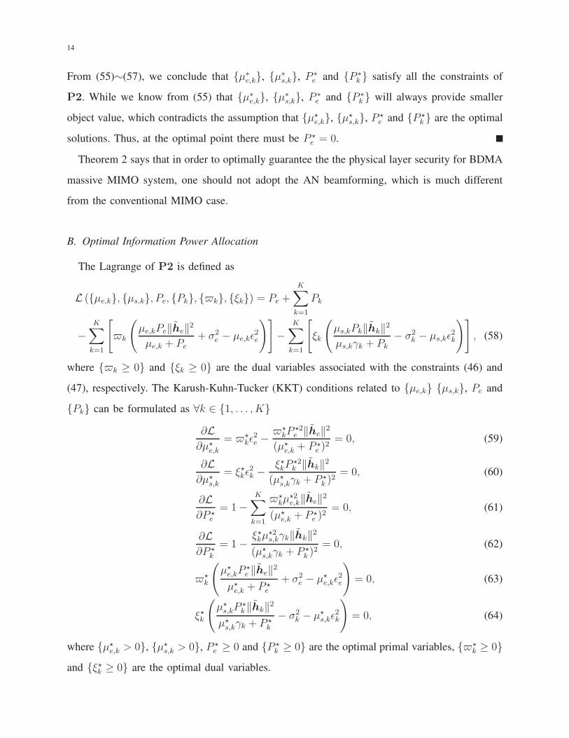
Fig. 2. Average SINR of Eve versus the parameter g with K = 30 and N = 128.

allocation for AN beamforming should be zero, which implies that the received SINR of Eve is

smaller than γe (please cf. Eq. (8) for details) without using AN. These theoretical results can

be reflected in Fig. 2 where it is clear that the average SINRs of Eve obtained by the proposed

method, the AN 6= 0 method and the non-robust method are smaller than 0 dB when g ≤ 0.7.

This phenomenon implies that the constraint in (8) will be strictly satisfied when we set γe > 0

dB. Based on the results of Fig. 2, we could always choose a small γe, i.e., 0 < γe < 1 to

guarantee that (8) is strictly satisfied for the proposed robust design. Moreover, it is obvious in

Fig. 2 that the average SINRs of Eve derived by the three methods will increase with the increase

of g. This is mainly due to the fact that when g becomes large, i.e., the channel estimation errors

grow large, more power will be received at Eve. Nevertheless, we can assume that g is a small

constant which is reasonable since large channel estimate errors usually lead to unacceptable

degradation in performance. It is seen from Fig. 2 that the average SINR of Eve derived by the

proposed method is always bigger than that of the AN 6= 0 method and the non-robust method.

This phenomenon can be explained by the following simulation results, i.e., the proposed method

will obtain a higher secret sum-rate.

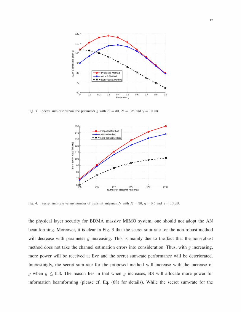
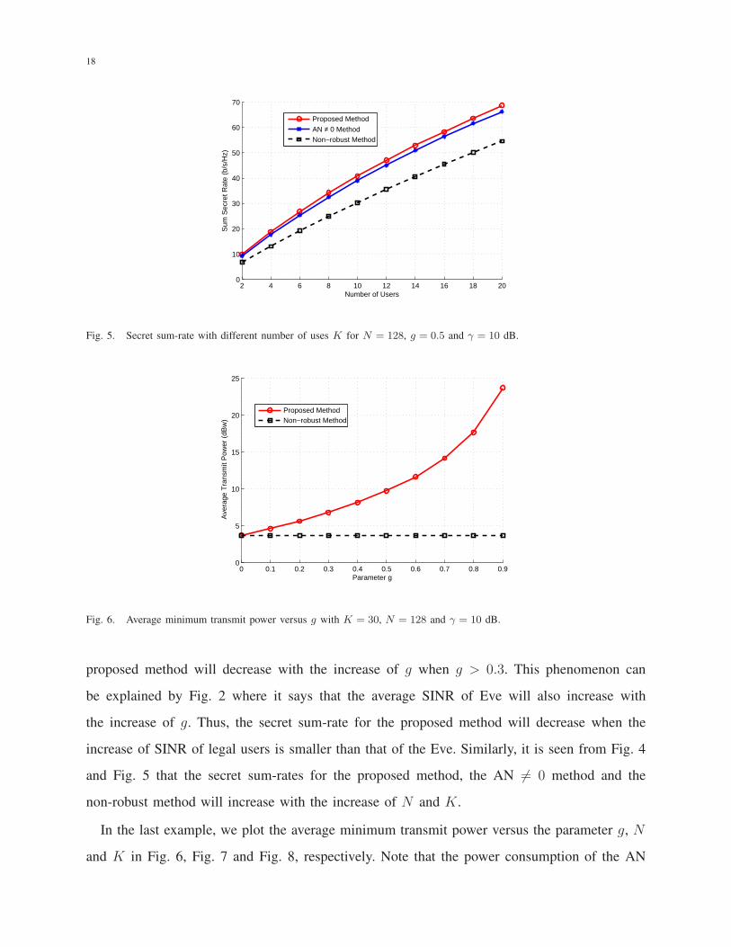
In the second example, we plot the secret sum-rate versus parameter g, N and K, in Fig. 3,

Fig. 4 and Fig. 5, respectively. Note that the secret sum-rate derived by the proposed method

is always bigger than that of the AN 6= 0 method. Thus, in order to optimally guarantee the

17

0 0.1 0.2 0.3 0.4 0.5 0.6 0.7 0.8 0.960

70

80

90

100

110

120

Parameter g

Sum

Sec

ret R

ate

(b/s

/Hz)

Proposed Method

AN ≠ 0 MethodNon−robust Method

Fig. 3. Secret sum-rate versus the parameter g with K = 30, N = 128 and γ = 10 dB.

2^5 2^6 2^7 2^8 2^9 2^1060

70

80

90

100

110

120

130

140

150

Number of Transmit Antennas

Sum

Sec

ret R

ate

(b/s

/Hz)

Proposed Method

AN ≠ 0 MethodNon−robust Method

Fig. 4. Secret sum-rate versus number of transmit antennas N with K = 30, g = 0.5 and γ = 10 dB.

the physical layer security for BDMA massive MIMO system, one should not adopt the AN

beamforming. Moreover, it is clear in Fig. 3 that the secret sum-rate for the non-robust method

will decrease with parameter g increasing. This is mainly due to the fact that the non-robust

method does not take the channel estimation errors into consideration. Thus, with g increasing,

more power will be received at Eve and the secret sum-rate performance will be deteriorated.

Interestingly, the secret sum-rate for the proposed method will increase with the increase of

g when g ≤ 0.3. The reason lies in that when g increases, BS will allocate more power for

information beamforming (please cf. Eq. (68) for details). While the secret sum-rate for the

18

2 4 6 8 10 12 14 16 18 200

10

20

30

40

50

60

70

Number of Users

Sum

Sec

ret R

ate

(b/s

/Hz)

Proposed Method

AN ≠ 0 MethodNon−robust Method

Fig. 5. Secret sum-rate with different number of uses K for N = 128, g = 0.5 and γ = 10 dB.

0 0.1 0.2 0.3 0.4 0.5 0.6 0.7 0.8 0.90

5

10

15

20

25

Parameter g

Ave

rage

Tra

nsm

it P

ower

(dB

w)

Proposed MethodNon−robust Method

Fig. 6. Average minimum transmit power versus g with K = 30, N = 128 and γ = 10 dB.

proposed method will decrease with the increase of g when g > 0.3. This phenomenon can

be explained by Fig. 2 where it says that the average SINR of Eve will also increase with

the increase of g. Thus, the secret sum-rate for the proposed method will decrease when the

increase of SINR of legal users is smaller than that of the Eve. Similarly, it is seen from Fig. 4

and Fig. 5 that the secret sum-rates for the proposed method, the AN 6= 0 method and the

non-robust method will increase with the increase of N and K.

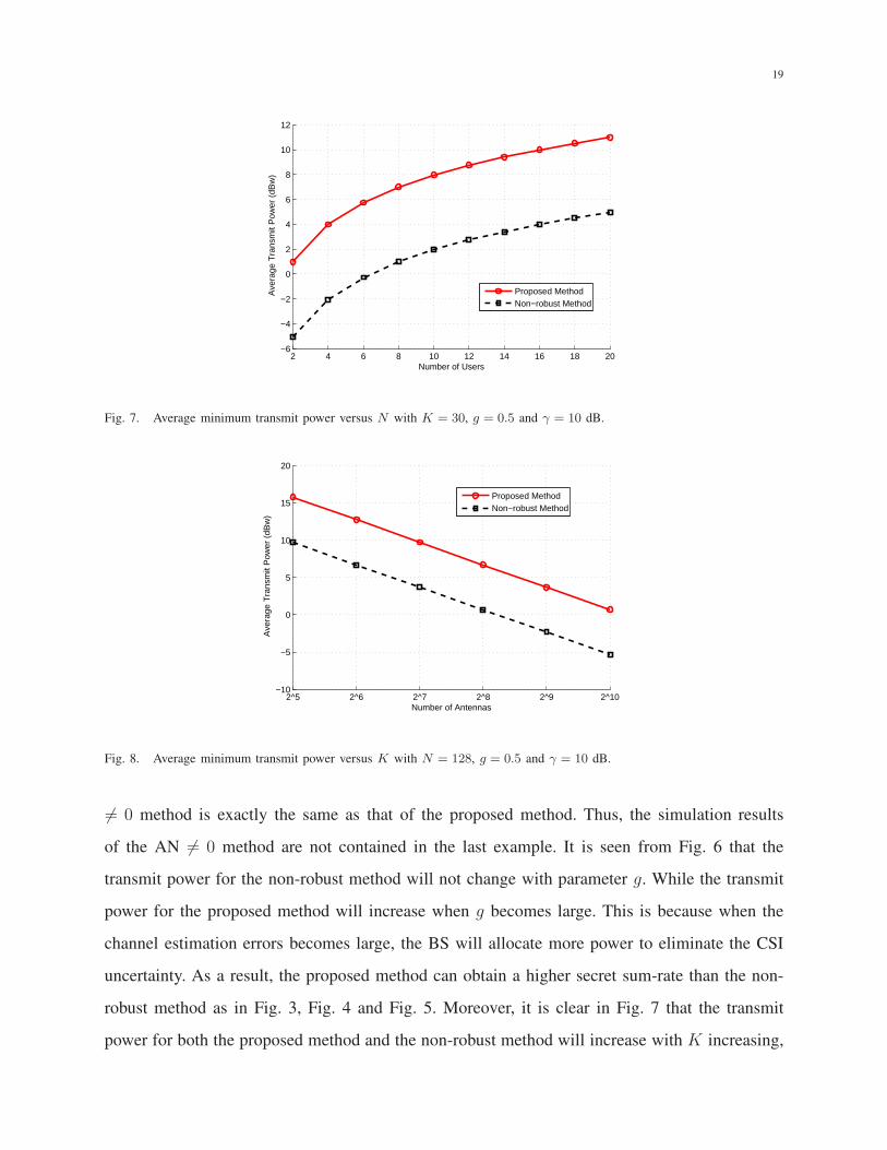
In the last example, we plot the average minimum transmit power versus the parameter g, N

and K in Fig. 6, Fig. 7 and Fig. 8, respectively. Note that the power consumption of the AN

19

2 4 6 8 10 12 14 16 18 20−6

−4

−2

0

2

4

6

8

10

12

Number of Users

Ave

rage

Tra

nsm

it P

ower

(dB

w)

Proposed MethodNon−robust Method

Fig. 7. Average minimum transmit power versus N with K = 30, g = 0.5 and γ = 10 dB.

2^5 2^6 2^7 2^8 2^9 2^10−10

−5

0

5

10

15

20

Number of Antennas

Ave

rage

Tra

nsm

it P

ower

(dB

w)

Proposed MethodNon−robust Method

Fig. 8. Average minimum transmit power versus K with N = 128, g = 0.5 and γ = 10 dB.

6= 0 method is exactly the same as that of the proposed method. Thus, the simulation results

of the AN 6= 0 method are not contained in the last example. It is seen from Fig. 6 that the

transmit power for the non-robust method will not change with parameter g. While the transmit

power for the proposed method will increase when g becomes large. This is because when the

channel estimation errors becomes large, the BS will allocate more power to eliminate the CSI

uncertainty. As a result, the proposed method can obtain a higher secret sum-rate than the non-

robust method as in Fig. 3, Fig. 4 and Fig. 5. Moreover, it is clear in Fig. 7 that the transmit

power for both the proposed method and the non-robust method will increase with K increasing,

20

and in Fig. 8 that the transmit power for both the proposed method and the non-robust method

will decrease with the increase of N .

VI. CONCLUSIONS

In this paper, we design simultaneous information and AN beamforming to guarantee the

physical layer security for multiuser BDMA massive MIMO systems. Taking the the channel

estimation errors into consideration, our target is to minimize the transmit power of BS meanwhile

provide the legal users and the Eve with different SINRs. The original problem is NP-hard and op-

timal solutions are generally unavailable in conventional communication systems. Nevertheless, it

is strictly proved that the initial non-convex optimization can be equivalently reformulated as an

SDP, where rank-one solutions are guaranteed in BDMA multiuser massive MIMO systems. More

importantly, the overall global optimal solutions for the original problem are derived in closed-

form, which will greatly reduce the computational complexity. An interesting phenomenon is

that the AN is not useful for multi-user BDMA massive scenario. Simulation results are provided

to corroborate the proposed studies.

APPENDIX A

PROOF OF PROPOSITION 1

A. Proof of Part (a)

Let us first show that {µ⋆e,k > 0} must hold from contradiction. Assuming µ⋆

e,k = 0 for some

k that k ∈ {1, . . . , K}, it follows from (20) that

Υe,k =

Xe,k Xe,khe

hHe X

He,k hH

e Xe,khe + σ2e

� 0 (A.1)

must be satisfied. Then it is obvious in (A.1) that

Xe,k =∑

i 6=k

Si +We −1

γe,kSk � 0, (A.2)

must be satisfied. Moreover, from (20) and (21) , we can obtain

Xs,k = −Xe,k − (1

γe,k−

1

γk)Sk � 0, (A.3)

where the last “�” holds true due to the fact that Xe,k � 0, Sk � 0 and γe,k < γk.

21

Next, we know from (19) that

hHkXs,khk − σ2

k − µs,kǫ2k ≥ 0, (A.4)

should be strictly satisfied. However, substituting (A.3) into (A.4), we will obtain

0 ≤ hHkXs,khk − σ2

k − µs,kǫ2k ≤ −σ2

k − µs,kǫ2k ≤ −σ2

k, (A.5)

where the last “≤” is satisfied since µs,k ≥ 0 and ǫ2k > 0. Due to the fact that σ2k > 0, we know

from (A.5) can not be true. Thus, at the optimal point, µ⋆e,k > 0, ∀k ∈ {1, . . . , K} must be

satisfied in P1−SDR.

B. Proof of Part (b)

Then, let us show that {µ⋆s,k > 0} must hold from contradiction. Assuming µ⋆

s,k = 0 for some

k that k ∈ {1, . . . , K}, it follows from (21) that

Υs,k =

Xs,k Xs,khk

hHkX

Hs,k hH

kXs,khk − σ2k

� 0, (A.6)

must be satisfied. Left and right multiplying both sides of Υs,k by [−hHk 1] and [−hH

k 1]H,

respectively, yields

[−hHk 1]Υs,k[−hH

k 1]H = −σ2k ≥ 0, (A.7)

which cannot be true due to σ2k > 0. Thus, at the optimal point, µ⋆

s,k > 0, ∀k ∈ {1, . . . , K}

must be satisfied in P1−SDR.

The proof is thus completed.

APPENDIX B

PROOF OF PROPOSITION 2

A. Proof of Part (a)

Let us show that Rank(

X⋆e,k + µ⋆

e,kI)

≥ 1, ∀k ∈ {1, . . . , K} from contradiction. Assume

Rank(

X⋆e,k + µ⋆

e,kI)

= 0 or X⋆e,k + µ⋆

e,kI = 0 at the optimal point, for some k that ∀k ∈

{1, . . . , K}. It is known from (21) that X⋆e,k + µ⋆

e,kI can be re-expressed as

X⋆e,k + µ⋆

e,kI = µ⋆e,kI +

∑

i 6=k

S⋆i +W ⋆

e −1

γe,kS⋆

k = 0. (B.1)

22

From Proposition 1, we know that µ⋆e,k > 0 is strictly satisfied at the optimal point. Moreover,

due to the fact that {S⋆k � 0} and W ⋆

e � 0, there must be

Rank

(

µ⋆e,kI +

∑

i 6=k

S⋆i +W ⋆

e

)

= N, (B.2)

which says that µ⋆e,kI +

∑

i 6=k

S⋆i + W ⋆

e ≻ 0. Then from (B.1) and (B.2) we know that when

X⋆e,k + µ⋆

e,kI = 0, there must be S⋆k ≻ 0 or Rank (S⋆

k) = N .

Define N ×N matrix Q as

Q =

[

he

‖he‖,

h1

‖h1‖, . . . ,

hK

‖hK‖, τ1, . . . , τN−K−1

]

, (B.3)

where τN×1i , ∀i ∈ {1, . . . , N −K − 1} is a unit vector, i.e., ‖τi‖ = 1 which is constrained to

satisfy the following properties:

(a) τi ⊥ τj , ∀i 6= j;

(b) τi ⊥ he, ∀i ∈ {1, . . . , N −K − 1};

(c) τi ⊥ hk, ∀i ∈ {1, . . . , N −K − 1}, ∀k ∈ {1, . . . , K}.

Thanks to (1) under BDMA massive MIMO scheme, we know that the defined matrix Q is

consisted of N orthogonal bases. Thus, Q is invertible, i.e., Q−1 exists. Consequently, there

must be

Rank (QW ⋆e ) = Rank (W ⋆

e ) , (B.4)

Rank (QS⋆k) = Rank (S⋆

k) , ∀k ∈ {1, . . . , K}. (B.5)

From (B.3), (B.4) and (B.5), we know that W ⋆e and S⋆

k , ∀k ∈ {1, . . . , K} can be further expressed

as

W ⋆e = P ⋆

we,he

hehHe

‖he‖2+

K∑

i=1

P ⋆we,hi

hihHi

‖hi‖2+

N−K−1∑

i=1

P ⋆we,τi

τiτHi , (B.6)

S⋆k = P ⋆

sk,he

hehHe

‖he‖2+

K∑

i=1

P ⋆sk,hi

hihHi

‖hi‖2+

N−K−1∑

i=1

P ⋆sk,τi

τiτHi , (B.7)

where P ⋆we,he

≥ 0, {P ⋆we,hi

≥ 0}, {P ⋆we,τi

≥ 0}, P ⋆sk,he

≥ 0, {P ⋆sk,hi

≥ 0} and {P ⋆sk,τi

≥ 0}. Note

that if Rank (S⋆k) = N , then there must be P ⋆

sk,he> 0, {P ⋆

sk,hi> 0} and {P ⋆

sk,τi> 0}. Under the

previous assumption, there is at least one S⋆k that satisfies Rank (S⋆

k) = N , where P ⋆sk,he

> 0,

{P ⋆sk,hi

> 0} and {P ⋆sk,τi

> 0} must hold.

23

Then, letting {P ⋆we,τi

= 0}, {P ⋆sk,τi

= 0}, ∀i ∈ {1, . . . , N −K − 1}, ∀k ∈ {1, . . . , K}, we can

construct the following new solutions

W ∗e = P ⋆

we,he

hehHe

‖he‖2+

K∑

i=1

P ⋆we,hi

hihHi

‖hi‖2,

S∗k = P ⋆

sk,he

hehHe

‖he‖2+

K∑

i=1

P ⋆sk,hi

hihHi

‖hi‖2.

(B.8)

Substituting (B.8) into P1−SDR and using the properties of (B.3), we obtain

Tr(W ⋆e ) +

K∑

k=1

Tr(S⋆k) > Tr(W ∗

e ) +

K∑

k=1

Tr(S∗k) (B.9)

X∗e,k + µ⋆

e,kI X∗e,khe

hHe X

∗He,k hH

e X∗e,khe + σ2

e − µ⋆e,kǫ

2e

� 0, (B.10)

X∗s,k + µ⋆

s,kI X∗s,khk

hHkX

∗Hs,k hH

kX∗s,khk − σ2

k − µ⋆s,kǫ

2k

� 0, (B.11)

X∗e,k =

∑

i 6=k

S∗i +W ∗

e −1

γe,kS∗

k , (B.12)

X∗s,k =

1

γkS∗

k −∑

i 6=k

S∗i −W ∗

e , (B.13)

µ⋆e,k ≥ 0, µ⋆

s,k ≥ 0, W ∗e � 0, S∗

k � 0, k = 1, 2, . . . , K. (B.14)

From (B.10)∼(B.14) we know that W ∗e and {S∗

k} satisfy all constraints of P1−SDR. From

(B.9) we know that W ∗e and {S∗

k} will always provide smaller objective value. Consequently,

W ∗e and {S∗

k} are better solutions than W ⋆e and {S⋆

k}, which contradicts with our first place as-

sumption. Thus, there must be Rank (S⋆k) < N and Rank

(

X⋆e,k + µ⋆

e,kI)

≥ 1, ∀k ∈ {1, . . . , K}.

B. Proof of Part (b)

Let us show that Rank(

X⋆s,k + µ⋆

s,kI)

≥ 1, ∀k ∈ {1, . . . , K} from contradiction. Assume

Rank(

X⋆s,k + µ⋆

s,kI)

= 0 or X⋆s,k + µ⋆

s,kI = 0 at the optimal point, for some k that ∀k ∈

{1, . . . , K}. Due to the fact that µ⋆s,k > 0, ∀k ∈ {1, . . . , K} (please cf. Proposition 1 for details),

there must be

X⋆k = −µ⋆

s,kI � 0. (B.15)

24

Then substituting (B.15) into (19), it is easily known that

0 X⋆s,khk

hHkX

⋆Hs,k hH

k (−µ⋆s,kI)hk − σ2

k − µ⋆s,kǫ

2k

� 0, (B.16)

must be strictly satisfied. which cannot be true due to the fact that hHk (−µ⋆

s,kI)hk−σ2k−µ⋆

s,kǫ2k <

0. Thus there must be Rank(

X⋆s,k + µ⋆

s,kI)

≥ 1, ∀k ∈ {1, . . . , K}.

The proof of Proposition 2 is completed.

APPENDIX C

PROOF OF THEOREM 1

The following lemma is useful in the proof of Theorem 1.

Lemma 3 (Theory of Majorization [33]): Let A and B be two N ×N positive semi-definite

matrices with eigenvalues α1 ≥ . . . ≥ αN and β1 ≥ . . . ≥ βN , respectively. Then there holds

N∑

i=1

αiβN−i+1 ≤ Tr(AB) ≤N∑

i=1

αiβi. (C.1)

Firstly, it follows from (B.8) that at the optimal point, W ⋆e and {S⋆

k} can be expressed as

W ⋆e = P ⋆

we,he

hehHe

‖he‖2+

K∑

i=1

P ⋆we,hi

hihHi

‖hi‖2,

S⋆k = P ⋆

sk,he

hehHe

‖he‖2+

K∑

i=1

P ⋆sk,hi

hihHi

‖hi‖2,

(C.2)

where P ⋆we,he

≥ 0 and {P ⋆we,hi

≥ 0} are the coefficients of W ⋆e , while P ⋆

sk,he≥ 0 and {P ⋆

sk,hi≥ 0}

are the coefficients of S⋆k. Then using (C.2), X⋆

e,k and X⋆s,k can be expressed as

X⋆e,k =

∑

i 6=k

S⋆i +W ⋆

e −1

γe,kS⋆

k (C.3)

=

(

∑

i 6=k

P ⋆si,he

+ P ⋆we,he

−1

γe,kP ⋆sk,he

)

hehHe

‖he‖2+

K∑

j=1

(

∑

i 6=k

P ⋆si,hj

+ P ⋆we,hj

−1

γe,kP ⋆sk,hj

)

hjhHj

‖hj‖2,

X⋆s,k =

1

γkS⋆

k −∑

i 6=k

S⋆i −W ⋆

e (C.4)

=

(

1

γkP ⋆sk,he

−∑

i 6=k

P ⋆si,he

− P ⋆we,he

)

hehHe

‖he‖2+

K∑

j=1

(

1

γkP ⋆sk,hj

−∑

i 6=k

P ⋆si,hj

− P ⋆we,hj

)

hjhHj

‖hj‖2.

With the BDMA massive MIMO regime, the estimated channel vectors satisfy hi ⊥ hk ⊥

he, ∀i 6= k. Thus, we know from (C.2)∼(C.4) that he/‖he‖, h1/‖h1‖, . . . , hK/‖hK‖ ∈ {ue,k,i}

25

and he/‖he‖, h1/‖h1‖, . . . , hK/‖hK‖ ∈ {us,k,i}, where ue,k,i and us,k,i are the ith column of

Ue,k and Us,k respectively. Based on the above discussions, we know from (41) that:

(a) If he/‖he‖ lies in the null space of X⋆e,k+µ⋆

e,kI , i.e., he/‖he‖ = ue,k,i and le,k+1 ≤ i ≤ N ,

there holds

∑

i 6=k

P ⋆si,he

+ P ⋆we,he

−1

γe,kP ⋆sk,he

+ µ⋆e,k = 0; (C.5)

(b) If he/‖he‖ lies in the range space of X⋆e,k+µ⋆

e,kI , i.e., he/‖he‖ = ue,k,i and 1 ≤ i ≤ le,k,

there holds

∑

i 6=k

P ⋆si,he

+ P ⋆we,he

−1

γe,kP ⋆sk,he

+ µ⋆e,k > 0. (C.6)

Similarly, we know from (42) that

(a) If hk/‖hk‖ lies in the null space of X⋆s,k+µ⋆

s,kI i.e., hk/‖hk‖ = us,k,i and ls,k+1 ≤ i ≤ N ,

there holds

1

γkP ⋆sk,hk

−∑

i 6=k

P ⋆si,hk

− P ⋆we,hk

+ µ⋆s,k = 0; (C.7)

(b) If hk/‖hk‖ lies in the range space of X⋆s,k+µ⋆

s,kI , i.e., hk/‖hk‖ = us,k,i and 1 ≤ i ≤ ls,k,

there holds

1

γkP ⋆sk,hk

−∑

i 6=k

P ⋆si,hk

− P ⋆we,hk

+ µ⋆s,k > 0. (C.8)

Next, let the EVD of He be He = Uh,eΛh,eUHh,e

, where Λh,e is diagonal with the eigenvalues

λe,1 ≥ . . . ≥ λe,N . Since He = hehHe has only one nonzero eigenvalue, there must be λe,1 > 0,

λe,2 = . . . = λe,N = 0 and uh,e,1 = he/‖he‖, where uh,e,1 is the first column of Uh,e. Then

according to (41) and Lemma 3, we know that (43) can be further reformulated as

0 ≤ Tr{(

HeXe,k

) [

I − (Xe,k + µe,kI)†Xe,k

]}

+ σ2e − µe,kǫ

2e

=Tr{(

He,kXe,k

) [

I − (Xe,k + µe,kI)† (Xe,k + µe,kI − µe,kI)

]}

+ σ2e − µe,kǫ

2e

=µe,kTr[

HeXe,k (Xe,k + µe,kI)†]

+ σ2e − µe,kǫ

2e

=µe,kTr

Λe,k

Σ−1e,k,+ 0

0 0

UHe,kUh,eΛh,eU

Hh,eUe,k

+ σ2e − µe,kǫ

2e

=µe,kqe,k,iλe,1

µe,k + qe,k,i+ σ2

e − µe,kǫ2e ≤

µe,kqe,k,1λe,1

µe,k + qe,k,1+ σ2

e − µe,kǫ2e, (C.9)

26

where qe,k,i is the ith eigenvalue of Xe,k whose corresponding eigenvector is ue,k,i = uh,e,1 =

he/‖he‖, and qe,k,1 is the maximum eigenvalue of Xe,k. Note that in (C.9), the last “≤” holds

with “=” when ue,k,1 = uh,e,1 = he/‖he‖.

Similarly, let the EVD of Hk be Hk = Uh,kΛh,kUHh,k

where Λh,k is diagonal with the single

non-zero eigenvalue λk,1 > 0 and the first column of Uh,k is uh,k,1 = hk/‖hk‖. According to

(42) and Lemma A, we know that (44) can be reformulated as (the details are omitted here for

brevity)

Tr{(

HkXs,k

) [

I − (Xs,k + µs,kI)†Xs,k

]}

− σ2k − µs,kǫ

2k

=µs,kqs,k,iλk,1

µs,k + qs,k,i− σ2

k − µs,kǫ2k ≤

µs,kqs,k,1λk,1

µs,k + qs,k,1− σ2

k − µs,kǫ2k, (C.10)

where qs,k,i is the ith eigenvalue of Xs,k whose corresponding eigenvector is us,k,i = uh,k,1 =

hk/‖hk‖, and qs,k,1 is the maximum eigenvalue of Xs,k. Note that in (C.10), the last “≤” holds

with “=” when us,k,1 = uh,k,1 = hk/‖hk‖, where us,k,1, uh,k,1 are the first columns of Us,k and

Uh,k respectively.

Lastly, let us show that Rank (W ⋆e ) ≤ 1 and Rank (S⋆

k) ≤ 1, ∀k ∈ {1, . . . , K} from contra-

diction. Assume {µ⋆e,k}, {µ⋆

s,k}, W ⋆e and {S⋆

k} are the optimal solutions of P1−SDR−EQV,

where Rank (W ⋆e ) = Ce > 1 or Rank (S⋆

k) = Ck > 1. Then we provide the following new

solutions

W ∗e =

(

P ⋆we,he

+

K∑

i=1

P ⋆si,he

)

hehHe

‖he‖2, S∗

k =

(

P ⋆sk,hk

−∑

i 6=k

P ⋆si,hk

− P ⋆we,hk

)

hkhHk

‖hk‖2, (C.11)

which satisfies Rank (W ∗e ) ≤ 1 and Rank (S∗

k) ≤ 1, ∀k ∈ {1, . . . , K}. Then it is obvious that

X∗e,k and X∗

s,k can be expressed as

X∗e,k =

∑

i 6=k

S∗i +W ∗

e −1

γe,kS∗

k =∑

i 6=k

(

P ⋆si,hi

−∑

j 6=i

P ⋆sj ,hi

− P ⋆we,hi

)

hihHi

‖hi‖2

+

(

P ⋆we,he

+

K∑

i=1

P ⋆si,he

)

hehHe

‖he‖2−

1

γe,k

(

P ⋆sk,hk

−∑

i 6=k

P ⋆si,hk

− P ⋆we,hk

)

hkhHk

‖hk‖2, (C.12)

X∗s,k =

1

γkS∗

k −∑

i 6=k

S∗i −W ∗

e =1

γk

(

P ⋆sk,hk

−∑

i 6=k

P ⋆si,hk

− P ⋆we,hk

)

hkhHk

‖hk‖2

−∑

i 6=k

(

P ⋆si,hi

−∑

j 6=i

P ⋆sj ,hi

− P ⋆we,hi

)

hihHi

‖hi‖2−

(

P ⋆we,he

+

K∑

i=1

P ⋆si,he

)

hehHe

‖he‖2, (C.13)

27

respectively. From (C.3) and (C.12), we know

∑

i 6=k

P ⋆si,he

+ P ⋆we,he

−1

γe,kP ⋆sk,he

≤ P ⋆we,he

+K∑

i=1

P ⋆si,he

, (C.14)

which implies that W ∗e and {S∗

k} will not violate the constraints in (34) of P1−SDR−EQV

(please cf. Eq. (C.5) and Eq. (C.6) for details). From (C.4) and (C.13), we obtain

1

γkP ⋆sk,hk

−∑

i 6=k

P ⋆si,hk

− P ⋆we,hk

≤1

γk

(

P ⋆sk,hk

−∑

i 6=k

P ⋆si,hk

− P ⋆we,hk

)

, (C.15)

which implies that W ∗e and {S∗

k} will not violate the constraints in (36) of P1−SDR−EQV

(please cf. Eq. (C.7) and Eq. (C.8) for details). Moreover, it is easily known from (C.3), (C.4),

(C.12) and (C.13) that if µ⋆s,k −

(

P ⋆we,he

+∑K

i=1 P⋆si,he

)

≥ 0, there must hold X∗e,k + µ⋆

e,kI � 0

and X∗s,k + µ⋆

s,kI � 0. Interestingly, it is observed from (C.9) that we can always let qe,k,1 =

P ⋆we,he

+∑K

i=1 P⋆si,he

= 0 and µe,k = σ2e/ǫ

2e, which will not violate (C.9). A more rigorous proof

can be found in Theorem 2.

As a result, substituting W ∗e and {S∗

k} into P1−SDR−EQV, we obtain from (32) that

Tr(W ∗e )+

K∑

k=1

Tr(S∗k)=P ⋆

we,he+

K∑

i=1

P ⋆si,he

+K∑

k=1

(

P ⋆sk,hk

−∑

i 6=k

P ⋆si,hk

− P ⋆we,hk

)

≤P ⋆we,he

+

K∑

i=1

P ⋆si,he

+

K∑

k=1

P ⋆sk,hk

+

K∑

j=1

K∑

i=1

P ⋆si,hj

=Tr(W ⋆e )+

K∑

k=1

Tr(S⋆k); (C.16)

from (33) and (34) that

X∗e,k + µ⋆

e,kI � 0, X∗s,k + µ⋆

s,kI � 0; (C.17)[

I −(

X∗e,k + µ⋆

e,kI) (

X∗e,k + µ⋆

e,kI)†]

X∗e,khe = 0; (C.18)

from (35) that

Tr{(

HeX∗e,k

) [

I −(

X∗e,k + µ⋆

e,kI)†X∗

e,k

]}

+ σ2e − µ⋆

e,kǫ2e

=µe,k

(

P ⋆we,he

+∑K

i=1 P⋆si,he

)

λe,1

µe,k + P ⋆we,he

+∑K

i=1 P⋆si,he

+ σ2e − µ⋆

e,kǫ2e

≥

µe,k

(

∑

i 6=k

P ⋆si,he

+ P ⋆we,he

−1

γe,kP ⋆sk,he

)

λe,1

µe,k +∑

i 6=k

P ⋆si,he

+ P ⋆we,he

−1

γe,kP ⋆sk,he

+ σ2e − µ⋆

e,kǫ2e

=Tr{(

HeX⋆e,k

) [

I −(

X⋆e,k + µe,kI

)†X⋆

e,k

]}

+ σ2e − µ⋆

e,kǫ2e > 0; (C.19)

28

from (36) that

[

I −(

X∗s,k + µ⋆

s,kI) (

X∗s,k + µ⋆

s,kI)†]

X∗s,khk = 0; (C.20)

from (37) that

Tr{(

HkX∗s,k

) [

I −(

X∗s,k + µ⋆

s,kI)†X∗

s,k

]}

− σ2k − µ⋆

s,kǫ2k

=µ⋆s,k

(

P ⋆sk,hk

−∑

i 6=k P⋆si,hk

− P ⋆we,hk

)

/γkλk,1

µ⋆s,k +

(

P ⋆sk,hk

−∑

i 6=k P⋆si,hk

− P ⋆we,hk

)

/γk− σ2

k − µ⋆s,kǫ

2k

≥µ⋆s,k

(

P ⋆sk,hk

/γk −∑

i 6=k P⋆si,hk

− P ⋆we,hk

)

λk,1

µ⋆s,k + P ⋆

sk,hk/γk −

∑

i 6=k P⋆si,hk

− P ⋆we,hk

− σ2k − µ⋆

s,kǫ2k

=Tr{(

HkX⋆s,k

) [

I −(

X⋆s,k + µ⋆

s,kI)†X⋆

s,k

]}

− σ2k − µ⋆

s,kǫ2k > 0; (C.21)

from (38), (39) and (40) that

X∗e,k =

∑

i 6=k

S∗i +W ∗

e −1

γe,kS∗

k , X∗s,k =

1

γkS∗

k −∑

i 6=k

S∗i −W ∗

e ; (C.22)

µ⋆e,k ≥ 0, µ⋆

s,k ≥ 0, W ∗e � 0, S∗

k � 0, k = 1, 2, . . . , K. (C.23)

Then it can be inferred from (C.16)∼(C.23) that

(a) If Rank (W ⋆e ) = Ce > 1, we know from (C.2) that there exists at least one P ⋆

we,hi>

0, i ∈ {1, . . . , K}. Thus, from (C.16)∼(C.20), (C.22) and (C.23) we know that W ∗e and

{S∗k} will not change the object value (32) and always satisfy constraints (33)∼(36) and

(38)∼(40). While from (C.21) we know that W ∗e and {S∗

k} will always provide more

freedoms. Thus, W ∗e and {S∗

k} are better solutions than W ⋆e and {S⋆

k}.

(b) If Rank (S⋆k) = Ck > 1, we know from (C.2) that there exists at least one P ⋆

sk,hi6=k>

0, i ∈ {1, . . . , K} or P ⋆sk,he

> 0. Then, if P ⋆sk,hi6=k

> 0, i ∈ {1, . . . , K}, we know from

(C.16) that W ∗e and {S∗

k} will always provide smaller objective value than W ⋆e and {S⋆

k}.

While from (C.17)∼(C.23), we know that W ∗e and {S∗

k} satisfy all the constraints of

P1−SDR−EQV. Thus, W ∗e and {S∗

k} are better solutions. If P ⋆sk,he

> 0, we know

from (C.16)∼(C.18) and (C.20)∼(C.23) that W ∗e and {S∗

k} will not change the object

value (32) and always satisfy constraints (33), (34) and (36)∼(40). While from (C.19) we

conclude that W ∗e and {S∗

k} will always provide more freedoms. Thus, W ∗e and {S∗

k} are

better solutions than W ⋆e and {S⋆

k}.

29

Based on the above discussions, we know that W ∗e and {S∗

k} are always better solutions,

which contradicts the assumption that W ⋆e and {S⋆

k} are optimal solutions. Thus there must

be Rank (W ⋆e ) ≤ 1 and Rank (S⋆

k) ≤ 1, ∀k ∈ {1, . . . , K}. From (C.11), we know W ⋆e and

{S⋆k} can be further expressed as

W ∗e = P ⋆

we

hehHe

‖he‖2, S∗

k = P ⋆sk

hkhHk

‖hk‖2, (C.24)

where P ⋆we

and P ⋆sk

are the optimal power allocation for AN beamforming and information

beamforming, respectively. The proof of Theorem 1 is thus completed.

REFERENCES

[1] T. L. Marzetta, “Noncooperative cellular wireless with unlimited nnumbers of base station antennas,” IEEE Trans. Wireless

Commun., vol. 9, no. 11, pp. 3590–3600, Nov. 2010.

[2] J. G. Andrews, S. Buzzi, W. Choi, S. V. Hanly, A. Lozano, A. C. Soong, and J. C. Zhang, “What will 5G be?” IEEE J.

Sel. Areas Commun., vol. 32, no. 6, pp. 1065–1082, Jun. 2014.

[3] E. G. Larsson, O. Edfors, F. Tufvesson and T. L. Marzetta, “Massive MIMO for next generation wireless systems,” IEEE

Commun. Mag., vol. 52, no. 2, pp. 186–195, Feb. 2014.

[4] L. Lu, G. Y. Li, A. L. Swindlehurst, A. Ashikhmin and R. Zhang, “An overview of massive MIMO: Benefits and challenges,”

IEEE J. Sel Topics Signal Process., vol. 8, no. 5, pp. 742–758, Oct. 2014.

[5] H. Yin, D. Gesbert, M. Filippou, and Y. Liu, “A coordinated approach to channel estimation in large-scale multiple-antenna

systems,” IEEE J. Sel. Areas Commun., vol. 31, no. 2, pp. 264–273, Feb. 2013.

[6] A. Adhikary, J. Nam, J.-Y. Ahn, and G. Caire, “Joint spatial division and multiplexing the large scale array regime,” IEEE

Trans. Inf. Theory, vol. 59, no. 10, pp. 6441–6463, Oct. 2013.

[7] H. Xie, B. Wang, F. Gao, S. Jin, “A full-space spectrum-sharing strategy for massive MIMO cognitive radio systems,”

IEEE J. Sel. Areas Commun., vol. 34, no. 10, pp. 2537-2549, Oct. 2016.

[8] H. Xie, F. Gao, S. Jin, “An overview of low-rank channel estimation for massive MIMO systems,” IEEE Access, vol. 4,

pp. 7313–7321, Nov. 2

[9] H. Xie, F. Gao, S. Zhang, S. Jin, “A unified transmission strategy for TDD/FDD massive MIMO systems with spatial basis

expansion model,” to appear in IEEE Trans. Veh. Technol., early access available online, 2016.

[10] W. Choi, A. Forenza, J. G. Andrews, and J. R. W. Heath, “Opportunistic space-division multiple access with beam selection,”

IEEE Trans. Commun., vol. 55, no. 12, pp. 2371–2380, Dec. 2007.

[11] C. Sun, X. Gao, S. Jin, M. Matthaiou, Z. Ding and C. Xiao, “Beam division multiple access transmission for massive

MIMO communications,” IEEE Trans. Commun., vol. 63, no. 6, pp. 2170-2184, June 2015.

[12] A. D. Wyner, “The wire-tap channel,” Bell Syst. Tech. J., vol. 54, pp. 1355–1387, Oct. 1975.

[13] I. Csiszar and J. Korner, “Broadcast channels with confidential messages,” IEEE Trans. Inf. Theory, vol. 24, no. 3, pp. 339–

348, May 1978.

30

[14] Y. Liang, H. V. Poor, and S. Shamai, “Secure communication over fading channels,” IEEE Trans. Inf. Theory, vol. 54,

no. 6, pp. 2470–2492, June 2008.

[15] Y. Liang and H. V. Poor, “Generalized multiple access channels with confidential messages,” in Proc. IEEE ISIT, Seattle,

WA, USA, July 2006, pp. 952–956.

[16] F. Oggier and B. Hassibi, “The secrecy capacity of the MIMO wiretap channel,” IEEE Trans. Inf. Theory, vol. 57, no. 8,

pp. 4961–4972, Aug. 2011.

[17] J. Zhu, R. Schober, and V. K. Bhargava, “Secure transmission in multicell massive MIMO systems,” IEEE Trans. Wireless

Commun., vol. 13, no. 9, pp. 4766–4781, Sep. 2014.

[18] X. Chen, L. Lei, H. Zhang, and C. Yuen, “Large-scale MIMO relaying techniques for physical layer security: AF or DF?”

IEEE Trans. Wireless Commun., vol. 14, no. 9, pp. 5135C5146, Sep. 2015.

[19] J. Wang, J. Lee, F. Wang and T. Q. S. Quek, “Jamming-aided secure communication in massive MIMO rician channels,”

IEEE Trans. Wireless Commun., vol. 14, no. 12, pp. 6854–6868, Dec. 2015.

[20] H. M. Wang, T. X. Zheng, J. Yuan, D. Towsley, and M. H. Lee, “Physical layer security in heterogeneous cellular networks,”

IEEE Trans. Wireless Commun., vol. 64, no. 3, pp. 1204–1219, Mar. 2016.

[21] J. Zhu, R. Schober, and V. K. Bhargava, “Linear precoding of data and artificial noise in secure massive MIMO systems,”

IEEE Trans. Wireless Commun., vol. 15, no. 3, pp. 2245–2261, Mar. 2016.

[22] Y. Wu, R. Schober, D. W. K. Ng, C. Xiao and G. Caire, “Secure massive MIMO transmission with an active eavesdropper,”

IEEE Trans. Inf. Theory, vol. 62, no. 7, pp. 3880–3900, July 2016.

[23] S. Boyd and L. Vandenberghe, Convex Optimization. Cambridge, U.K.: Cambridge University Press, 2004.

[24] X. Li, T. Jiang, S. Cui, J. An, and Q. Zhang, “Cooperative communications based on rateless network coding in distributed

MIMO systems,” IEEE Trans. Wireless Commun., vol. 17, no. 3, pp. 60–67, June 2010.

[25] Y. Rong, S. A. Vorobyov and A. B. Gershman, “Robust linear receivers for multiaccess space-time block-coded MIMO

systems: A probabilistically constrained approach,” IEEE J. Sel. Areas Commun., vol. 24, no. 8, pp. 1560–1570, Aug.

2006.

[26] J. Wang and D. P. Palomar, “Worst-Case Robust MIMO Transmission With Imperfect Channel Knowledge,” IEEE Trans.

Signal Process., vol. 57, no. 8, pp. 3086–3100, Aug. 2009.

[27] N. Vucic and H. Boche, “Robust QoS-Constrained Optimization of Downlink Multiuser MISO Systems,” IEEE Trans.

Signal Process., vol. 57, no. 2, pp. 714–725, Feb. 2009.

[28] A. Mostafa and L. Lampe, “Optimal and robust beamforming for secure transmission in MISO visible-light communication

links,” IEEE Trans. Signal Process., vol. 64, no. 24, pp. 6501–6516, Dec. 2016.

[29] S. Boyd, L. E. Ghaoui, E. Feron, and V. Balakrishnan, Linear Matrix Inequalities in System and Control Theory.

Philadelphia, PA: SIAM Studies in Applied Mathematics, 1994.

[30] Z. Q. Luo, W. K. Ma, A. M. C. So, Y. Ye, and S. Zhang, “Semidefinite relaxation of quadratic optimization problems,”

IEEE Signal Process. Mag., vol. 27, no. 3, pp. 20–34, May 2010.

[31] R. Penrose, “A generalized inverse for matrices,” in Proc. Cambridge Philos. Soc., 1955, vol. 51, pp. 406–413.

[32] R. A. Horn and C. R. Johnson, Matrix Analysis. New York: Cambridge University Press, 1985.

[33] A. W. Marshall and I. Olkin, Inequalities: Theory of Majorization and Its Applications. New York: Academic, 1979.