1

Robust and practical analog-to-digital conversionwith exponential precision

Ingrid Daubechies andOzgur Yılmaz

Abstract

Beta-encoders with error correction were introduced by Daubechies, DeVore, Gunturk and Vaishampayan as analternative to PCM for analog-to-digital conversion. A beta-encoder quantizes a real number by computing one ofits N -bit truncatedβ-expansions whereβ ∈ (1, 2) determines the base of expansion. These encoders have (almost)optimal rate-distortion properties like PCM; furthermorethey exploit the redundancy of beta-expansions and thusthey are robust with respect to quantizer imperfections. However, these encoders have the shortcoming that thedecoder needs to know the value of the base of expansionβ, a gain factor in the circuit used by the encoder,which is an impractical constraint. We present a method to implement beta-encoders so that they are also robustwith respect to uncertainties of the value ofβ. The method relies upon embedding the value ofβ in the encodedbitstream. We show that this can be done without a priori knowledge ofβ by the transmitting party. Moreover thealgorithm still works if the value ofβ changes (slowly) during the implementation.

Index Terms

A/D conversion, beta-encoders, beta-expansions, quantization, sampling, sigma-delta

I. INTRODUCTION

Analog-to-digital (A/D) conversion consists of two steps:samplingand quantization. We shall assume thatf ,the analog signal of interest, is a bandlimited function, i.e., its Fourier transformf vanishes outside a boundedinterval. In this case, the standard sampling theorem states that we can reconstruct the signal from its sample valueson a sufficiently dense grid. In particular, if the support off is contained in[−Ω,Ω], the sequencef(nπ/Ω)n∈Z

determinesf via

f(t) =∑

n

f(nπ

Ω) sinc (

Ωt

π− n). (1)

In practice, (1) is not very useful because the “sinc kernel”decays slowly, and thus the reconstruction is not local.However, we can overcome this problem by sampling on a densergrid, in which case we can replace the sinc in(1) by a kernel with much faster decay. In particular, if instead of the sample sequencef(nπ/Ω)n∈Z the moreclosely-spaced samplesf(nπ/(λΩ))n∈Z (with λ > 1) are used, (1) can be replaced by

f(t) =1

λ

∑

n

f(nπ

λΩ) ϕ(

Ωt

π−

n

λ), (2)

whereϕ is any function such thatϕ(ξ) = 1 for |ξ| ≤ Ω and ϕ(ξ) = 0 for |ξ| ≥ λΩ. If, in addition, we chooseϕsuch thatϕ is smooth,ϕ will have the desired decay properties.

The second step in A/D conversion isquantization, which will be our focus in this paper. Quantization is thereplacement of the sample valuesf(nπ/(λΩ)) in the reconstruction formula (2) by numbers from a discrete(usuallyfinite) set. Unlike sampling, quantization is not an invertible operation. Therefore, aquantization schemeis usuallydescribed by a pair of mappings, an encoderE and a decoderD. The encoderE maps functions of interest tobitstreams; the decoderD aims to invertE as “closely” as possible. In general, however,D(Ef) 6= f .

Ingrid Daubechies is with the Department of Mathematics andwith the Program in Applied and Computational Mathematics,PrincetonUniversity

Ozgur Yılmaz is with the Department of Mathematics, The University of British Columbia.Ingrid Daubechies was partially suported by NSF Grant DMS-0219233 and by AFOSR Grant F49620-01-0099.Ozgur Yılmaz was partially

supported by the Natural Science and Engineering Research Council of Canada.

2

In this paper, we focus on quantization algorithms for functions in S(Ω,M), the class of functions inL2(R)with L∞-norm bounded byM , and with Fourier transforms supported in[−Ω,Ω]. When considering functions inS(Ω,M) we shall refer to any interval of lengthπ/Ω as aNyquist interval. In what follows we shall consider,without loss of generality, only the caseΩ = π andM = 1, and denoteS(π, 1) by S. For any quantization scheme,or, equivalently, for any encoder-decoder pair(E,D), we define thedistortion d by

d(S;E,D) := supf∈S

‖f − D(Ef)‖ (3)

where‖ · ‖ is the norm of interest. The performance of a quantization scheme onS is typically characterized bythe relation between the distortiond and the numberB of bits per Nyquist interval consumed (on average) bythe encoderE associated with the quantization scheme; we call this number the bit budgetof the quantizationscheme. A typical way of comparing the performances of two quantization schemes is to compare the bit budgetsthey utilize to produce approximations with the same amountof distortion; if no other considerations prevail, thequantization scheme with the smaller bit budget is superior, and is preferable. Equivalently, one might comparethe distortions associated with several quantization schemes for the same fixed bit budget; in this case, the schemewith the smaller distortion is favored.

One widely used quantization scheme ispulse code modulation(PCM). Given a functionf in S, anN -bit PCMalgorithm simply replaces each sample valuef(n/λ) with N bits: one bit for its sign, followed by the firstN − 1bits of the binary expansion of|f(n/λ)|. One can show that for signals inS this algorithm achieves a precisionof order O(2−N ); i.e., for f in S, the distortiond(f ;E,D) ≤ C2−N when (E,D) is the encoder-decoder pairassociated with anN -bit PCM, and when the norm‖ · ‖ to measure the distortion is either theL∞ norm onR, orthe limit, asT → ∞, of the normalizedL2-norm (2T )−1/2‖ · ‖L2(−T,T ). This can also be rephrased in terms of thebit-budget: since the average number of bits per Nyquist interval isB := Nλ, we haved(f,E,D) ≤ Cλ2−B/λ forf ∈ S, whereλ > 1 can be chosen arbitrarily, withCλ ≤ C ′(λ − 1)−1/2 tending to∞ asλ → 1.

On the other hand,sigma-delta modulation, another commonly implemented quantization algorithm forfunctionsin S, achieves a precision that decays like only an inverse polynomial in the bit budgetB. For example, akth-ordersigma-delta scheme produces an approximation where theL∞ approximation error (i.e., distortion) is of orderO(B−k).

Despite their clearly inferior performance in terms of distortion for a given bit budget, sigma-delta modulatorsare oftenpreferredover PCM for A/D conversion of audio signals in practice. This must mean that other factors aremore important. A plausible explanation for the prevalenceof sigma-delta modulators is given by the robustnessproperties of these schemes, when implemented in analog circuits. Every quantization scheme for analog-to-digitalconversion must contain (at least one) nonlinear “decisionelement” that “performs the quantization”, i.e., transformsits real number input into an element of a (finite) alphabet; we shall call this nonlinear element thequantizer,reserving this name for this use only. These quantizers are bound to be imprecise, i.e., the location of their “togglepoint(s)” is typically not known with high precision. Underthese circumstances, PCM performs poorly whereasthe distortion associated with a sigma-delta scheme is hardly affected at all [1]; more precisely, the error made bya PCM quantization scheme with an imprecise quantizer is bounded below by a strictly positive constant (directlyrelated to the measure of imprecision of the quantizer), whereas the error made by akth order sigma-delta schemestill decays likeB−k, and therefore can be made arbitrarily small despite the imprecision in the quantizer.

One of several reasons why sigma-delta schemes are robust isthat they quantize redundant expansions of theoriginal function. Since redundant expansions are not unique, any error caused by an imprecise quantizer can beimplicitly corrected later. This is clearly not the case forPCM, since the binary expansion of almost every realnumber is unique, and therefore a bit flip in the expansion cannot be corrected by changes in the consecutive bits.For a detailed discussion of robustness properties of sigma-delta schemes as well as a comparison with PCM, werefer to [2], [3], [1], [4].

It is natural to wonder whether we can have the best of both worlds. In other words, can we construct aquantization algorithm that utilizes the bit-budget efficiently, like PCM, but that is at the same time robust withrespect to unavoidable imprecision errors in the (analog) circuit implementation, like sigma-delta modulators? In[1] two quantization schemes are discussed that show that the answer to this question is affirmative: a modified,filtered sigma-delta scheme, first proposed in [5], and a scheme that is introduced in [1] for the first time (as far aswe know), called a “beta-encoder with error correction”. These beta-encoders are PCM-like in that they quantize

3

each sample finely and achieve exponential precision for theresulting approximation; moreover they are robust,like sigma-delta schemes, because this fine quantization isdone in a redundant way.

Although the encoders discussed in [1] are robust against quantizer imperfections, they nevertheless still havecertain robustness problems, at least from a practical point of view. Both of them use other parameters (the filterparameters for the scheme of [5], the factorβ used in the beta-encoder) that need to be implemented with highaccuracy. In this paper, we shall discuss this issue furtherfor beta-encoders.

The beta-encoder of [1], which we outline in Section II, computes a “truncatedβ-ary expansion” for each samplevalue, i.e., a series expansion in a baseβ, where1 < β < 2, and with binary coefficients. In order to reconstruct agood approximation to the original signal value from these binary coefficients, it is crucial to know the value ofβ,with a precision comparable to at least the one we hope the quantization scheme to achieve. However, measuring theexact value ofβ as well as ensuring that it stays constant over a long stretchof time is difficult, if not impossible,in an analog setting.

In this paper, we show how this obstacle can be circumvented.We present an algorithm that encodes and transmitsthe value ofβ without in fact physically measuring its value. This is doneby embedding the value ofβ in theencoded bitstream for each sample value separately. Thus weconstruct a beta-encoder that is not only robust toquantizer imperfections, but also robust with respect toβ, as long as the value ofβ remains constant or variessufficiently slowly that it does not change by more than the desired precision range of the quantization schemeover, say, twenty sampling intervals.

In Section II we outline the “beta-encoders with error correction”, introduced in [1]. In Section III we present our“beta-robust” approach and prove that it has the robustnessproperties discussed above. In Section IV we presentnumerical examples and consider some variations to our approach that address other robustness concerns.

II. REVIEW OF BETA-ENCODERS

In this section, we summarize certain properties of beta-encoders with error correction. See [1] for more details.We start again from the observation that any functionf ∈ S can be reconstructed from its sample valuesf(n/λ)via

f(t) = λ−1∑

n

f(n

λ) ϕ(t −

n

λ). (4)

whereλ > 1 andϕ ∈ C∞, such thatϕ(ξ) = 1 for |ξ| ≤ π and ϕ(ξ) = 0 for |ξ| ≥ λπ.

Proposition 1. Let f ∈ S, ǫ > 0 and consider any quantization scheme that producesqn such thatsup |f(n/λ)−qn| ≤ ǫ. Then the approximationf , defined as

f(t) := λ−1∑

n

qn ϕ(t −n

λ) (5)

satisfies|f(t) − f(t)| ≤ λ−1

∑

n

ǫ |ϕ(t −n

λ)| ≤ Cϕ ǫ (6)

whereCϕ := ‖ϕ‖L1 + λ−1‖ϕ′‖L1

Proposition 1 shows, for example, that if theqn are produced by anN -bit PCM algorithm, then the functionfdefined by (5) satisfies

‖f − f‖L∞ ≤ Cϕ2−N+1, (7)

because, by construction, anN -bit PCM generatesqn such that|f(n/λ) − qn| ≤ 2−N+1 for all n.Next, we will consider, instead of truncated binary expansions, truncated 1-bitβ expansions of the sample values.

By a 1-bit β expansionwe mean an expansion with binary coefficients and baseβ ∈ (1, 2). For any real numberx ∈ [0, 1], and given1 < β ≤ 2, there exists a sequence(bj)j∈N, with bj ∈ 0, 1 such that

x =∞∑

j=1

bjβ−j . (8)

4

Clearly, for β = 2, (8) corresponds to the binary expansion ofx; for 1 < β < 2, the expansion is said to be abeta-expansion, and is not unique; in fact, for every1 < β < 2 and for almost everyx in (0, 1], the set of differentβ expansions ofx has the cardinality of the continuum [6].

Given x ∈ [0, 1], one way to compute a binary sequencebj that satisfies (8) is to run the iteration

uj = β(uj−1 − bj−1)

bj = Q(uj) (9)

with u1 = βx, and

Q(u) :=

1 u > 10 u ≤ 1 .

(10)

The nonlinear operationQ in (10) is an idealized quantizer; in practice one has to dealwith quantizers that onlyapproximate this ideal behavior (see below). The samplesf(n/λ) of a functionf ∈ S will be real numbers in(−1, 1)rather than(0, 1); we shall here perform a small “sleight of hand” and considerthe value-shifted and renormalizedfunction g = (f + 1)/2 instead, which does take values in(0, 1) only. Running (9)N times for each sample valueg(n/λ) = [1 + f(n/λ)]/2, wheref ∈ S, will yield an N -bit truncated beta-expansionqn :=

∑Nj=1 bjβ

−j thatwill satisfy

|g(n/λ) − qn| < Cβ−N or |f(n/λ) − (2qn − 1)| < C ′β−N (11)

whereC ′ = 2C = 2/(β − 1). Thus, by Proposition 1, such a quantization scheme will yield an approximation tof ∈ S with distortion of sizeO(β−N ).

Before defining the “beta-encoders with error correction” of [1], we want to repeat the key observation that isused in [1] to construct these encoders.

Proposition 2. Let x ∈ (0, 1) and b1, b2, . . . , bJ be arbitrary such thatbj ∈ 0, 1. If

0 ≤ x −J

∑

j=1

bjβ−j ≤

1

βJ(β − 1)(12)

then there exists an extensionbj∞

j=J+1 such that

x =∞∑

j=1

bjβ−j (13)

This is exactly where redundancy comes into play: Forβ = 2, the only way the bitsb1, . . . , bK can satisfy (12)is by being the firstK bits of the binary expansion ofx. However, for1 < β < 2, this is not the case; one isallowed to “undershoot” (i.e., put to0 some of the bitsbj = 1 in the beta-expansion produced by (9) ) as long as(12) is satisfied. This means that the beta-encoder described by (9) is “semi-robust” in the sense that it can correctquantizer errors that result from underestimating certainbit values in the expansion.

This feature has the following important consequence in practice. When the beta-encoder runs the iterativealgorithm (9) to quantize a real number, the specific form (10) for the quantizerQ is difficult to implementprecisely. A more realistic model is obtained by replacingQ in (9) with Q(· + δ) whereδ is a quantity that isnot known exactly, but over the magnitude of which we have some control, e.g.|δ| < ǫ for a knownǫ. We shallcall a quantization scheme “robust” if the worst approximation error it produces can be made arbitrarily small byallowing a sufficiently large bit budget, even ifǫ > 0 is kept fixed. In the form described above, beta-encoders arerobust only for some rangeδcrit > δ ≥ 0 that is asymmetric with respect to0, which is the reason why we calledthem semi-robust. (More precisely, later bitsbℓ, with ℓ > j, automatically rectify the error made by assigning avalue0 to a bj when the “ideal” value ofbj, according to (9), should have been1. The opposite error, in whichthe value1 was erroneously assigned to abj that should have been0, does not get corrected by this scheme.)In [1] a modified version of the algorithm described by the recursion in (9) is introduced, which remedies thissituation, i.e., it is robust for both positive and negativesmall δ. The basic strategy of [1] is to replaceQ in (9)with Qµ := Q(· − µ), for some appropriateµ. This means that the quantizer prefers assigning 0 to assigning 1, inthose cases when perfect reconstruction with the remainingbits is not only possible but can even be done with acomfortable margin . This way a range forδ can be determined, symmetric with respect to0, as specified below

5

in Theorem 3, so that when the scheme is implemented withQµ(· − δ) instead ofQµ, one still has exponentiallyprecise reconstruction of the original sample value. More precisely,

Theorem 3. Let ǫ > 0 and x ∈ (0, 1). Suppose that in the beta-encoding ofx, the procedure(9) is followed, butthe quantizerQµ(· − δ) is used instead of the idealQ at each occurrence, with the values ofδ possibly varyingfrom onej to the next, but always satisfying|δ| < ǫ. Denote by(bj)j∈N the bit sequence produced by applying thisencoding to the numberx. If ǫ ≤ µ, andβ satisfies

1 < β <2 + µ + ǫ

1 + µ + ǫ, (14)

then for eachN ≥ 1,

|x −

N∑

j=1

bjβ−j | ≤ Cβ−N (15)

with C = 1 + µ + ǫ.

Theorem 3 is a slightly rephrased version of Theorem 4.1 in [1]; it shows that the “beta-encoder with offsetµ”has the desired robustness properties with respect to the quantizer functionQµ. However, there isstill one parameterin the iteration that must be known precisely to implement the “beta-encoder with offsetµ” and to reconstruct theoriginal signal from the encoded bitstream, namely the baseβ of the expansion. If we were to implement theencoder in an analog setting, it seems that we would have two choices: either make sureβ has a precise value,known to the decoding as well as the encoding party, or measure and transmitβ before sending the encoded bits.Neither is feasible in practice: measuring the value ofβ physically and transmitting it separately is another potentialsource for errors; moreover it would be very hard, if not impossible, to measureβ with great precision. On theother hand, implementing the beta-encoder with offsetµ in hardware with aprecise and fixedβ would be as costlyas implementing a high-precision PCM. In the next section wepropose a way to circumvent this problem.

III. T HE APPROACH

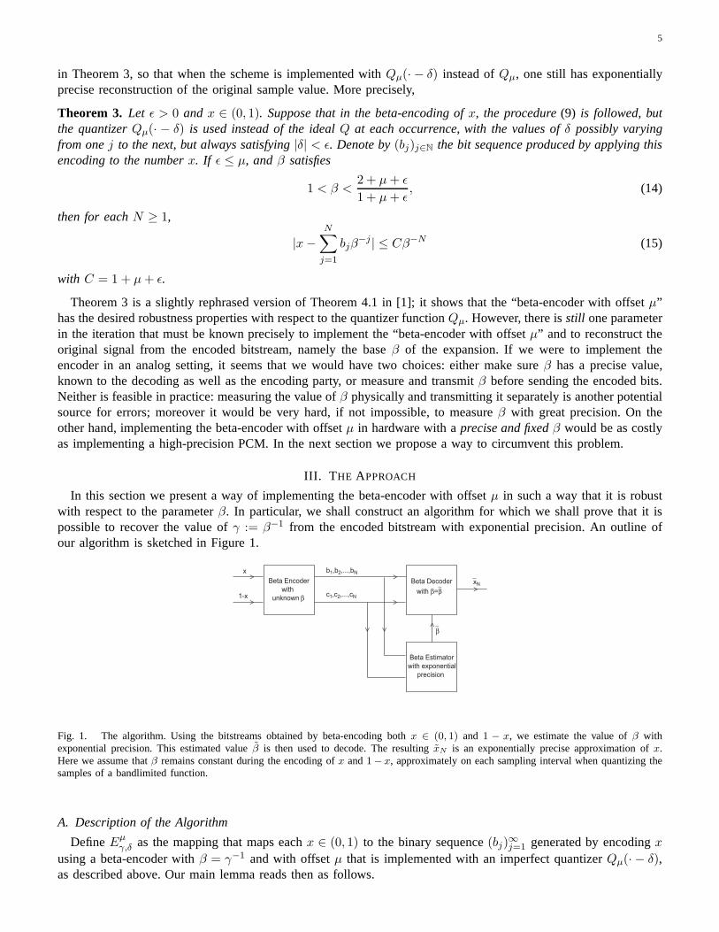
In this section we present a way of implementing the beta-encoder with offsetµ in such a way that it is robustwith respect to the parameterβ. In particular, we shall construct an algorithm for which weshall prove that it ispossible to recover the value ofγ := β−1 from the encoded bitstream with exponential precision. An outline ofour algorithm is sketched in Figure 1.

Beta Encoder

with

unknown β

x

1-x

b1,b2,...,bN

c1,c2,...,cN

Beta Decoder

with β=β∼

Beta Estimator

with exponential

precision

β∼

>

>

>

>

> >

>

∼xN

>

Fig. 1. The algorithm. Using the bitstreams obtained by beta-encoding bothx ∈ (0, 1) and 1 − x, we estimate the value ofβ withexponential precision. This estimated valueβ is then used to decode. The resultingxN is an exponentially precise approximation ofx.Here we assume thatβ remains constant during the encoding ofx and1− x, approximately on each sampling interval when quantizing thesamples of a bandlimited function.

A. Description of the Algorithm

DefineEµγ,δ as the mapping that maps eachx ∈ (0, 1) to the binary sequence(bj)

∞

j=1 generated by encodingxusing a beta-encoder withβ = γ−1 and with offsetµ that is implemented with an imperfect quantizerQµ(· − δ),as described above. Our main lemma reads then as follows.

6

Lemma 4. Let x ∈ (0, 1) and letγ = β−1 ∈ (1/2, 1) be such that(14) is satisfied, with0 < ǫ ≤ µ. Suppose|δ| < ǫ,and define the sequencesb := Eµ

γ,δ(x) and c := Eµγ,δ(1 − x). Let N be such thatmaxbj , cj : j = 1, . . . , N > 0.

Then, for anyγ that satisfies

0 ≤ 1 −N

∑

j=1

(bj + cj) γj ≤ 2 C γN , (16)

with C = 1 + µ + ǫ, we have|γ − γ| ≤ C ′γN , (17)

whereC ′ = max2C, 2C/(k0γ(k0−1)) with k0 =

log( 1−γ

2)

logγ .

We shall prove this lemma in several steps below. Before proceeding, we show that knowing the value ofγ withexponential precision yields exponentially precise approximations.

Theorem 5. Let x ∈ (0, 1), γ ∈ (1/2, 1) and (bj)j∈N ∈ 0, 1 be such thatx =∑

∞

j=1 bjγj. Supposeγ is such that

|γ − γ| ≤ C1γN for some fixedC1 > 0. DefineN0 := log[(1−γ)/C1]

log γ , and η := C1γN0+1. ThenxN :=

∑Nj=1 bj γ

j

satisfies the inequalities

|x − xN | ≤

C1γN 1

1−(γ+η)2 , N ≥ N0 + 1

C1γNN2

0 (γ + C1γ)N0−1, 1 ≤ N ≤ N0.(18)

Proof: We want to estimate

|x − xN | =

∣

∣

∣

∣

∣

∣

N∑

j=1

bj(γj − γj)

∣

∣

∣

∣

∣

∣

≤

N∑

j=1

|γj − γj | (19)

where we have used thatbj ∈ 0, 1. Define nowfj(γ) := γj − γj . Clearly, fj(γ) = 0; moreover the derivativesatisfies|f ′

j(γ)| = |jγj−1| ≤ j(γ + ∆)j−1 for all γ − ∆ ≤ γ ≤ γ + ∆, whereγ ∈ (1/2, 1) and∆ > 0. Therefore,

|fj(γ)| = |γj − γj| ≤ ∆j(γ + ∆)j−1. (20)

We will now estimate the right hand side of (19) separately for the cases whenN is large and whenN is small:1) Setting∆ = C1γ

N , and substituting (20) in (19), we get

|x − xN | ≤ C1γN

N∑

j=1

j(γ + C1γN )j−1 (21)

=C1γN 1 − (γ + C1γ

N )N (1 + N(1 − (γ + C1γN )))

(1 − (γ + C1γN ))2.

(22)

For N ≥ N0 + 1, C1γN ≤ C1γ

N0+1 = η; by its definitionη satisfiesη < 1 − γ, so that(γ + C1γN ) < 1.

We then rewrite (22) as

|x − xN | ≤ C1γN 1

(1 − (γ + C1γN ))2

≤ C1γN 1

(1 − (γ + η))2,

which provides us with the desired bound.2) Suppose that1 ≤ N ≤ N0, which means(γ + C1γ

N ) ≥ 1. Set again∆ = C1γN . For eachj = 1, . . . , N ,

we clearly have

|γj − γj| ≤ C1γNj(γ + C1γ

N )j−1

≤ C1γNN0(γ + C1γ)N0−1 (23)

where the second inequality holds becausej ≤ N ≤ N0 andN ≥ 1. Substituting (23) in (19), and using thatN ≤ N0 yields the desired estimate, i.e.,

|x − xN | ≤ γNC1N20 (γ + C1γ)N0−1.

7

Remarks:1) Combining Lemma 4 and Theorem 5, we see that one can recoverthe encoded numberx ∈ (0, 1) from the

first N bits of Eµγ,δ(x) andEµ

γ,δ(1 − x), with a distortion that decreases exponentially asN increases.2) Given N -bit truncated bitstreamsEµ

γ,δ(x) and Eµγ,δ(1 − x), one way to estimateγ is doing an exhaustive

search. Clearly this is computationally intensive. Note, however, that the search will be done in the digitaldomain, where computational constraints are not heavy, andcomputation speed is high.

3) In Section IV-B we introduce a fast algorithm that can replace exhaustive search; moreover its performanceis as good as exhaustive search.

B. Proof of the Main Lemma

In what follows, we shall present several observations thatlead us to a proof of Lemma 4 at the end of thesection.

Proposition 6. Let β ∈ (1, 2), γ := 1/β, and x ∈ (0, 1). Supposeµ, ǫ, and δ are such that the conditions ofTheorem 3 are satisfied. Letb := Eµ

γ,δ(x) and c := Eµγ,δ(1 − x). Then

0 ≤ 1 −N

∑

j=1

(bj + cj)γj ≤ 2CγN , (24)

whereC = 1 + µ + ǫ with |δ| < ǫ ≤ µ.

Proof: By Theorem 3, we know that

0 ≤ x −N

∑

j=1

bjγj ≤ CγN , (25)

and

0 ≤ 1 − x −

N∑

j=1

cjγj ≤ CγN (26)

hold. Combining (25) and (26) yields the result.

Note thatdj := bj +cj ∈ 0, 1, 2. Moreover, the index of the first non-zero entry ofdj∞

j=1 cannot be arbitrarilylarge; more precisely

Proposition 7. Let k := minj : j ∈ N and dj 6= 0. Then

k ≤log(1−γ

2 )

log γ. (27)

Proof: Let k be as defined above. Clearly, withdj = bj + cj as above,∞∑

j=k

djγj = 1. On the other hand, since

dj ∈ 0, 1, 2,∞∑

j=k

djγj ≤ 2

∞∑

j=k

γj =2γk

1 − γ. (28)

Therefore, we have2γk

1 − γ≥ 1, (29)

which yields the desired result.

8

−0.5 −0.4 −0.3 −0.2 −0.1 0 0.1 0.2 0.3 0.4−0.5

0

0.5

1

Fn

Gn

−t1

t0

t

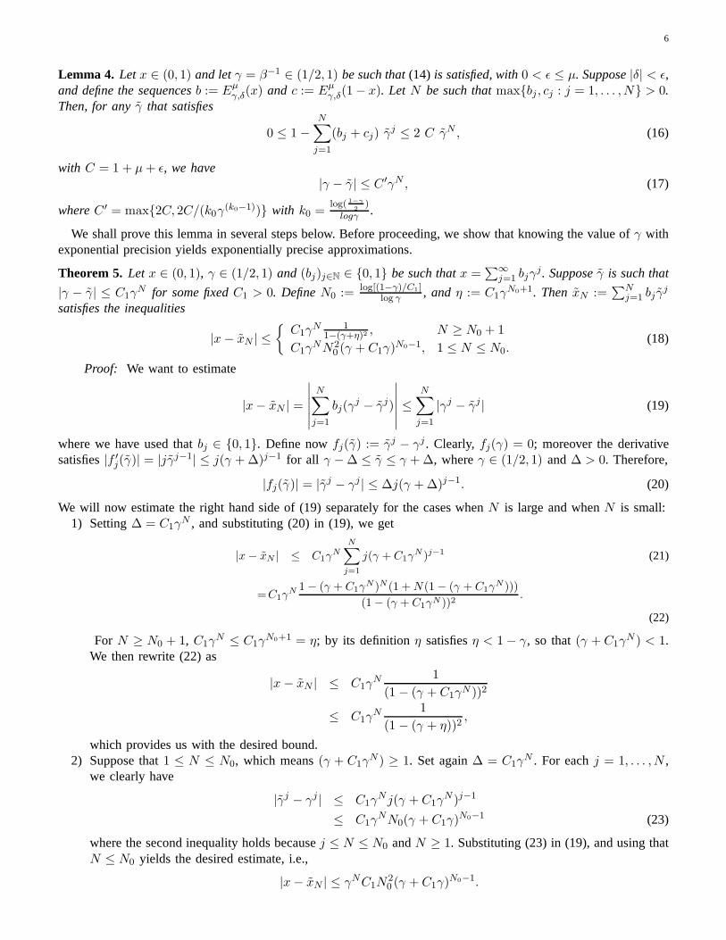
Fig. 2. A sketch of the graph ofFn along withGn(t) = 2C(γ + t)n. Heren = 5, andFn was computed via (30) from the firstn bits ofthe sequenceEµ

γ,δ(x) with x = 0.7, γ = 0.75, µ = 0.2, and |δ| < 0.1.

We now define

Fn(t) := 1 −

n∑

j=k

dj(γ + t)j (30)

on [−γ,∞) for n = k, k + 1, . . . .

Proposition 8. Fn has the following properties:

(i) 0 ≤ Fn(0) ≤ 2Cγn.(ii) Fn is monotonically decreasing. Moreover, the graph ofFn is concave for alln ∈ 2, 3, . . . .

Proof:

(i) This is Proposition 6 restated.

(ii) First, note thatF ′

n(t) = −

n∑

j=k

jdj(γ + t)j−1. Thus, sincedj ≥ 0 for all j, F ′

n(t) < 0 for t > −γ. Moreover,

a similar calculation shows that the second derivative ofFn is also negative. Therefore the graph ofFn isconcave.

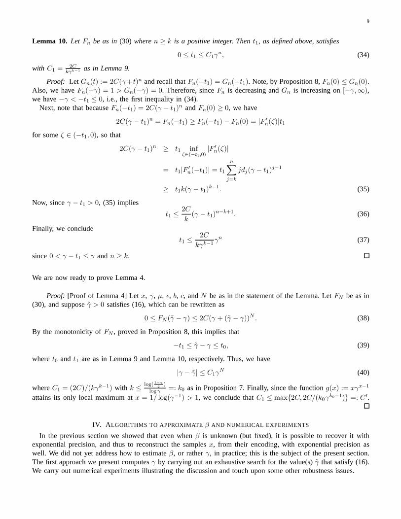
Figure 2 shows a sketch of the graph ofFn. Define, as shown in Figure 2,t0 as the point at whichFn(t0) = 0.Similarly, let t1 be such thatF (−t1) = 2C(γ − t1)

n. We will show that botht0 andt1 are at most of sizeO(γn),which will lead us to our main result.

Lemma 9. Let Fn be as in (30) wheren ≥ k is a positive integer. Thent0, as defined above, satisfies

0 ≤ t0 ≤ C1γn, (31)

with C1 = 2Ckγk−1 whereC is as in Theorem3 and k is as in Proposition7.

Proof: SinceFn is deceasing andFn(0) ≥ 0, it follows that t0 ≥ 0. MoreoverFn(0) = Fn(0) − Fn(t0) =|F ′

n(ξ)|t0 for someξ ∈ (0, t0), so that

t0 ≤ Fn(0)

[

infξ∈(0,t0)

|F ′

n(ξ)|

]

−1

≤ 2Cγn|F ′

n(0)|−1 . (32)

Finally, sinceF ′

n(0) = −

n∑

j=k

jdjγj−1 and sincedj ≥ 0, we have

|F ′

n(0)| ≥ kγk−1, (33)

wherek is as in Proposition 7. Combining (33) with (32) above yieldsthe result.

9

Lemma 10. Let Fn be as in(30) wheren ≥ k is a positive integer. Thent1, as defined above, satisfies

0 ≤ t1 ≤ C1γn, (34)

with C1 = 2Ckγk−1 as in Lemma 9.

Proof: Let Gn(t) := 2C(γ+ t)n and recall thatFn(−t1) = Gn(−t1). Note, by Proposition 8,Fn(0) ≤ Gn(0).Also, we haveFn(−γ) = 1 > Gn(−γ) = 0. Therefore, sinceFn is decreasing andGn is increasing on[−γ,∞),we have−γ < −t1 ≤ 0, i.e., the first inequality in (34).

Next, note that becauseFn(−t1) = 2C(γ − t1)n andFn(0) ≥ 0, we have

2C(γ − t1)n = Fn(−t1) ≥ Fn(−t1) − Fn(0) = |F ′

n(ζ)|t1

for someζ ∈ (−t1, 0), so that

2C(γ − t1)n ≥ t1 inf

ζ∈(−t1,0)|F ′

n(ζ)|

= t1|F′

n(−t1)| = t1

n∑

j=k

jdj(γ − t1)j−1

≥ t1k(γ − t1)k−1. (35)

Now, sinceγ − t1 > 0, (35) implies

t1 ≤2C

k(γ − t1)

n−k+1. (36)

Finally, we conclude

t1 ≤2C

kγk−1γn (37)

since0 < γ − t1 ≤ γ andn ≥ k.

We are now ready to prove Lemma 4.

Proof: [Proof of Lemma 4] Letx, γ, µ, ǫ, b, c, andN be as in the statement of the Lemma. LetFN be as in(30), and supposeγ > 0 satisfies (16), which can be rewritten as

0 ≤ FN (γ − γ) ≤ 2C(γ + (γ − γ))N . (38)

By the monotonicity ofFN , proved in Proposition 8, this implies that

−t1 ≤ γ − γ ≤ t0, (39)

wheret0 and t1 are as in Lemma 9 and Lemma 10, respectively. Thus, we have

|γ − γ| ≤ C1γN (40)

whereC1 = (2C)/(kγk−1) with k ≤log( 1−γ

2)

log γ =: k0 as in Proposition 7. Finally, since the functiong(x) := xγx−1

attains its only local maximum atx = 1/ log(γ−1) > 1, we conclude thatC1 ≤ max2C, 2C/(k0γk0−1) =: C ′.

IV. A LGORITHMS TO APPROXIMATEβ AND NUMERICAL EXPERIMENTS

In the previous section we showed that even whenβ is unknown (but fixed), it is possible to recover it withexponential precision, and thus to reconstruct the samplesx, from their encoding, with exponential precision aswell. We did not yet address how to estimateβ, or ratherγ, in practice; this is the subject of the present section.The first approach we present computesγ by carrying out an exhaustive search for the value(s)γ that satisfy (16).We carry out numerical experiments illustrating the discussion and touch upon some other robustness issues.

10

0 10 20 30

10−5

10−3

10−1

101

N

|γ−γN

| ~

(a)

0 10 20 30

10−5

10−3

10−1

101

N

|x−xN

| ~

(b)

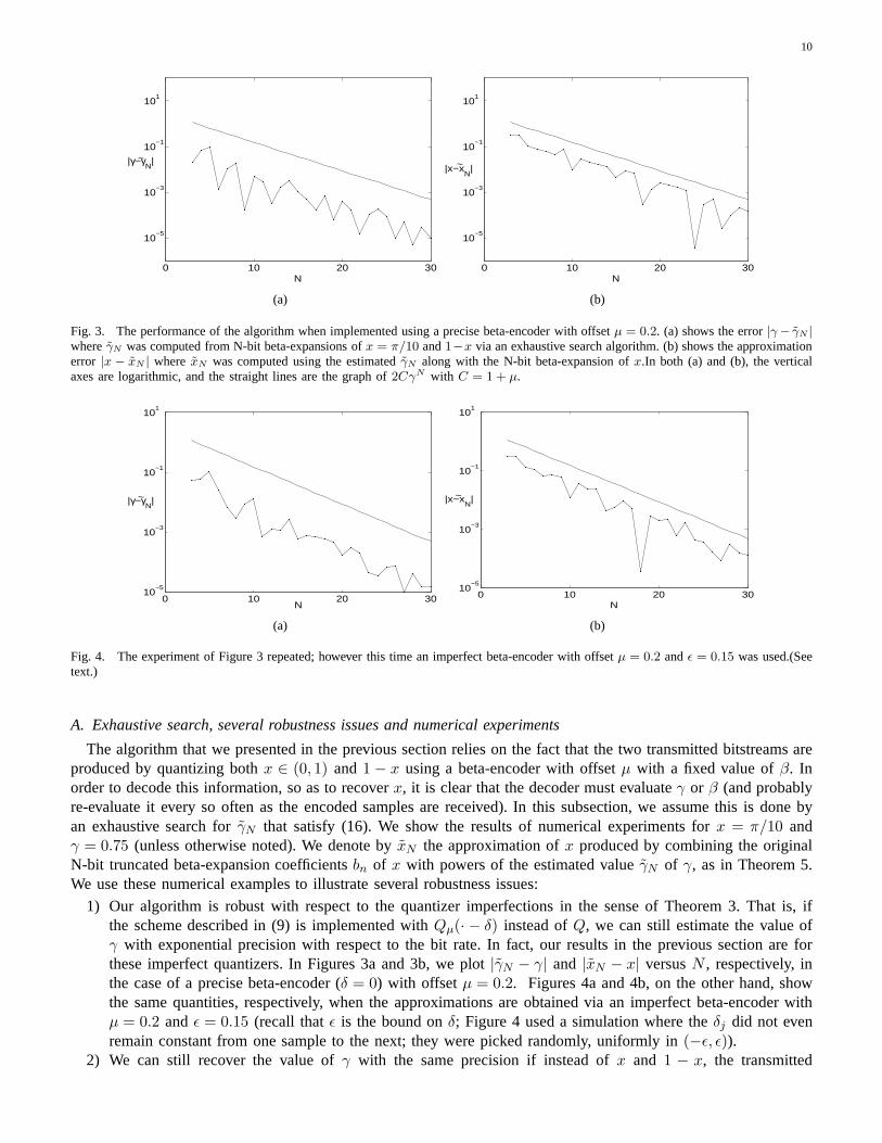
Fig. 3. The performance of the algorithm when implemented using a precise beta-encoder with offsetµ = 0.2. (a) shows the error|γ− γN |whereγN was computed from N-bit beta-expansions ofx = π/10 and1−x via an exhaustive search algorithm. (b) shows the approximationerror |x − xN | where xN was computed using the estimatedγN along with the N-bit beta-expansion ofx.In both (a) and (b), the verticalaxes are logarithmic, and the straight lines are the graph of2CγN with C = 1 + µ.

0 10 20 3010

−5

10−3

10−1

101

N

|γ−γN

|~

(a)

0 10 20 3010

−5

10−3

10−1

101

N

~ |x−xN

|

(b)

Fig. 4. The experiment of Figure 3 repeated; however this time an imperfect beta-encoder with offsetµ = 0.2 andǫ = 0.15 was used.(Seetext.)

A. Exhaustive search, several robustness issues and numerical experiments

The algorithm that we presented in the previous section relies on the fact that the two transmitted bitstreams areproduced by quantizing bothx ∈ (0, 1) and1 − x using a beta-encoder with offsetµ with a fixed value ofβ. Inorder to decode this information, so as to recoverx, it is clear that the decoder must evaluateγ or β (and probablyre-evaluate it every so often as the encoded samples are received). In this subsection, we assume this is done byan exhaustive search forγN that satisfy (16). We show the results of numerical experiments for x = π/10 andγ = 0.75 (unless otherwise noted). We denote byxN the approximation ofx produced by combining the originalN-bit truncated beta-expansion coefficientsbn of x with powers of the estimated valueγN of γ, as in Theorem 5.We use these numerical examples to illustrate several robustness issues:

1) Our algorithm is robust with respect to the quantizer imperfections in the sense of Theorem 3. That is, ifthe scheme described in (9) is implemented withQµ(· − δ) instead ofQ, we can still estimate the value ofγ with exponential precision with respect to the bit rate. In fact, our results in the previous section are forthese imperfect quantizers. In Figures 3a and 3b, we plot|γN − γ| and |xN − x| versusN , respectively, inthe case of a precise beta-encoder (δ = 0) with offset µ = 0.2. Figures 4a and 4b, on the other hand, showthe same quantities, respectively, when the approximations are obtained via an imperfect beta-encoder withµ = 0.2 andǫ = 0.15 (recall thatǫ is the bound onδ; Figure 4 used a simulation where theδj did not evenremain constant from one sample to the next; they were pickedrandomly, uniformly in(−ǫ, ǫ)).

2) We can still recover the value ofγ with the same precision if instead ofx and 1 − x, the transmitted

11

0 10 20 30

10−5

10−3

10−1

101

N

~ |γ−γN

|

(a)

0 10 20 30

10−3

10−1

101

N

|x−xN

| ~

(b)

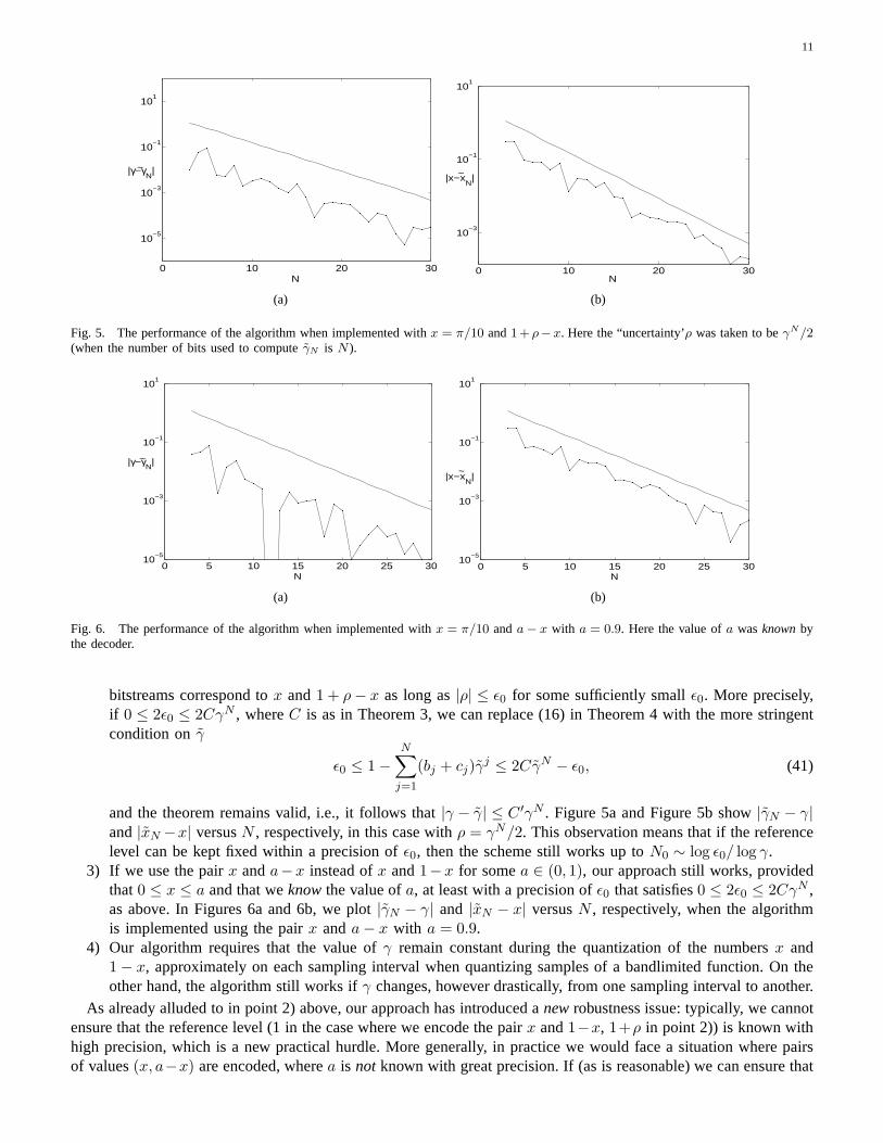
Fig. 5. The performance of the algorithm when implemented with x = π/10 and1+ ρ−x. Here the “uncertainty’ρ was taken to beγN/2(when the number of bits used to computeγN is N ).

0 5 10 15 20 25 3010

−5

10−3

10−1

101

N

|γ−γN

| ~

(a)

0 5 10 15 20 25 3010

−5

10−3

10−1

101

N

~ |x−x

N|

(b)

Fig. 6. The performance of the algorithm when implemented with x = π/10 anda − x with a = 0.9. Here the value ofa wasknownbythe decoder.

bitstreams correspond tox and1 + ρ − x as long as|ρ| ≤ ǫ0 for some sufficiently smallǫ0. More precisely,if 0 ≤ 2ǫ0 ≤ 2CγN , whereC is as in Theorem 3, we can replace (16) in Theorem 4 with the more stringentcondition onγ

ǫ0 ≤ 1 −N

∑

j=1

(bj + cj)γj ≤ 2CγN − ǫ0, (41)

and the theorem remains valid, i.e., it follows that|γ − γ| ≤ C ′γN . Figure 5a and Figure 5b show|γN − γ|and|xN −x| versusN , respectively, in this case withρ = γN/2. This observation means that if the referencelevel can be kept fixed within a precision ofǫ0, then the scheme still works up toN0 ∼ log ǫ0/ log γ.

3) If we use the pairx anda−x instead ofx and1−x for somea ∈ (0, 1), our approach still works, providedthat0 ≤ x ≤ a and that weknowthe value ofa, at least with a precision ofǫ0 that satisfies0 ≤ 2ǫ0 ≤ 2CγN ,as above. In Figures 6a and 6b, we plot|γN − γ| and |xN − x| versusN , respectively, when the algorithmis implemented using the pairx anda − x with a = 0.9.

4) Our algorithm requires that the value ofγ remain constant during the quantization of the numbersx and1 − x, approximately on each sampling interval when quantizing samples of a bandlimited function. On theother hand, the algorithm still works ifγ changes, however drastically, from one sampling interval to another.

As already alluded to in point 2) above, our approach has introduced anewrobustness issue: typically, we cannotensure that the reference level (1 in the case where we encodethe pairx and1−x, 1+ρ in point 2)) is known withhigh precision, which is a new practical hurdle. More generally, in practice we would face a situation where pairsof values(x, a−x) are encoded, wherea is not known with great precision. If (as is reasonable) we can ensure that

12

0.6 0.7 0.8 0.9

−0.8

−0.6

−0.4

−0.2

0

0.2

0.4

0.6

0.8

1

λ

p30

(x)

(a)

0.6 0.65 0.7 0.75 0.8−0.1

−0.05

0

0.05

0.1

λ

p30

(x)

(b)

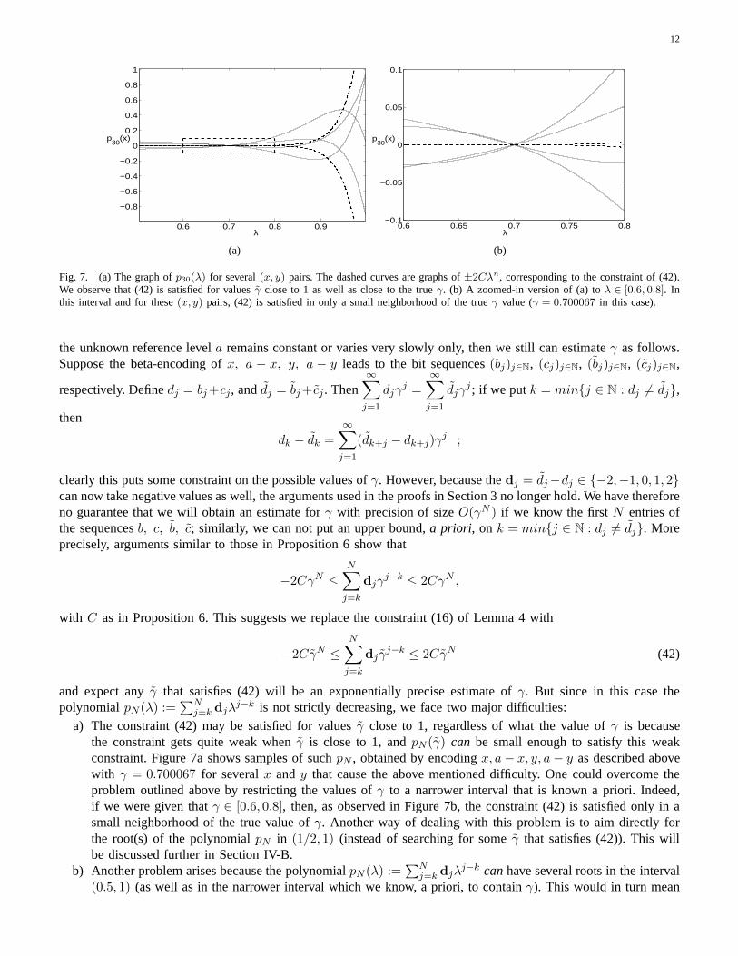
Fig. 7. (a) The graph ofp30(λ) for several(x, y) pairs. The dashed curves are graphs of±2Cλn, corresponding to the constraint of (42).We observe that (42) is satisfied for valuesγ close to 1 as well as close to the trueγ. (b) A zoomed-in version of (a) toλ ∈ [0.6, 0.8]. Inthis interval and for these(x, y) pairs, (42) is satisfied in only a small neighborhood of the true γ value (γ = 0.700067 in this case).

the unknown reference levela remains constant or varies very slowly only, then we still can estimateγ as follows.Suppose the beta-encoding ofx, a − x, y, a − y leads to the bit sequences(bj)j∈N, (cj)j∈N, (bj)j∈N, (cj)j∈N,

respectively. Definedj = bj +cj, anddj = bj + cj . Then∞∑

j=1

djγj =

∞∑

j=1

djγj ; if we putk = minj ∈ N : dj 6= dj,

then

dk − dk =

∞∑

j=1

(dk+j − dk+j)γj ;

clearly this puts some constraint on the possible values ofγ. However, because thedj = dj−dj ∈ −2,−1, 0, 1, 2can now take negative values as well, the arguments used in the proofs in Section 3 no longer hold. We have thereforeno guarantee that we will obtain an estimate forγ with precision of sizeO(γN ) if we know the firstN entries ofthe sequencesb, c, b, c; similarly, we can not put an upper bound,a priori, on k = minj ∈ N : dj 6= dj. Moreprecisely, arguments similar to those in Proposition 6 showthat

−2CγN ≤

N∑

j=k

djγj−k ≤ 2CγN ,

with C as in Proposition 6. This suggests we replace the constraint(16) of Lemma 4 with

−2CγN ≤

N∑

j=k

dj γj−k ≤ 2CγN (42)

and expect anyγ that satisfies (42) will be an exponentially precise estimate of γ. But since in this case thepolynomialpN (λ) :=

∑Nj=k djλ

j−k is not strictly decreasing, we face two major difficulties:

a) The constraint (42) may be satisfied for valuesγ close to 1, regardless of what the value ofγ is becausethe constraint gets quite weak whenγ is close to 1, andpN (γ) can be small enough to satisfy this weakconstraint. Figure 7a shows samples of suchpN , obtained by encodingx, a − x, y, a − y as described abovewith γ = 0.700067 for severalx andy that cause the above mentioned difficulty. One could overcome theproblem outlined above by restricting the values ofγ to a narrower interval that is known a priori. Indeed,if we were given thatγ ∈ [0.6, 0.8], then, as observed in Figure 7b, the constraint (42) is satisfied only in asmall neighborhood of the true value ofγ. Another way of dealing with this problem is to aim directly forthe root(s) of the polynomialpN in (1/2, 1) (instead of searching for someγ that satisfies (42)). This willbe discussed further in Section IV-B.

b) Another problem arises because the polynomialpN (λ) :=∑N

j=k djλj−k canhave several roots in the interval

(0.5, 1) (as well as in the narrower interval which we know, a priori, to containγ). This would in turn mean

13

0.6 0.65 0.7 0.75 0.8−0.04

0

0.04

0.08

λ

p30

(x)

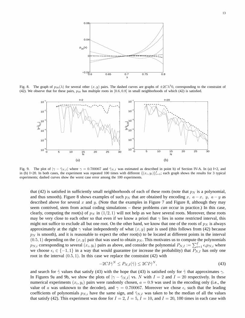
Fig. 8. The graph ofp30(λ) for several other(x, y) pairs. The dashed curves are graphs of±2Cλ30, corresponding to the constraint of(42). We observe that for these pairs,p30 has multiple roots in[0.6, 0.8] in small neighborhoods of which (42) is satisfied.

0 5 10 15 20 25 3010

−6

10−5

10−4

10−3

10−2

10−1

N

|γ−γ N

,2|

~

I=2

(a)

0 5 10 15 20 25 3010

−6

10−5

10−4

10−3

10−2

10−1

N

|γ−γ N

,20|

~

I=20

(b)

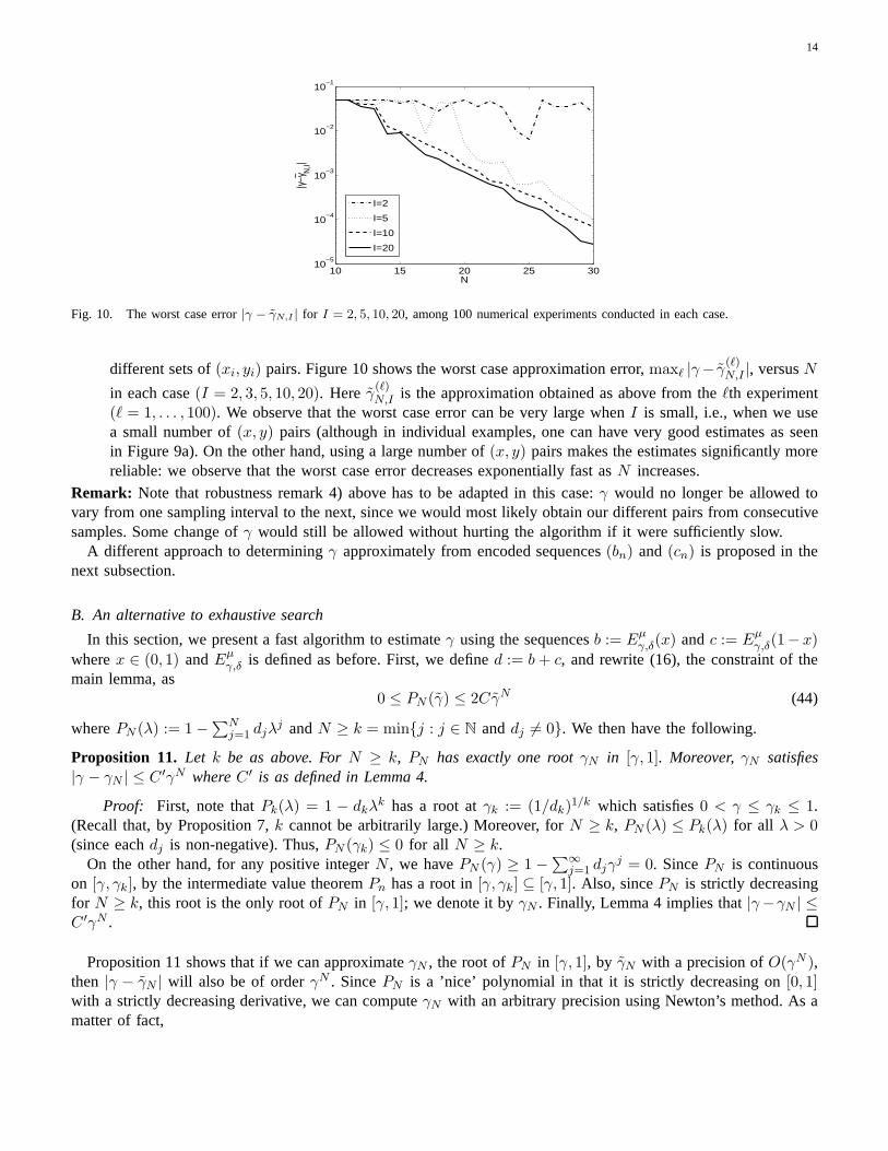
Fig. 9. The plot of|γ − γN,I | whereγ = 0.700067 and γN,I was estimated as described in point b) of Section IV-A. In (a)I=2, andin (b) I=20. In both cases, the experiment was repeated 100 times with different(xi, yi)

Ii=1; each graph shows the results for 3 typical

experiments; dashed curves show the worst case error among the 100 experiments.

that (42) is satisfied in sufficiently small neighborhoods ofeach of these roots (note thatpN is a polynomial,and thus smooth). Figure 8 shows examples of suchpN that are obtained by encodingx, a−x, y, a− y asdescribed above for severalx andy. (Note that the examples in Figure 7 and Figure 8, although they mayseem contrived, stem from actual coding simulations – theseproblemscan occur in practice.) In this case,clearly, computing the root(s) ofpN in (1/2, 1) will not help as we have several roots. Moreover, these rootsmay be very close to each other so that even if we know a priori that γ lies in some restricted interval, thismight not suffice to exclude all but one root. On the other hand, we know that one of the roots ofpN is alwaysapproximately at the rightγ value independently of what(x, y) pair is used (this follows from (42) becausepN is smooth), and it is reasonable to expect the other root(s) to be located at different points in the interval(0.5, 1) depending on the(x, y) pair that was used to obtainpN . This motivates us to compute the polynomialspN,i corresponding to several(xi, yi) pairs as above, and consider the polynomialPN,I :=

∑Ii=1 ǫipN,i where

we chooseǫi ∈ −1, 1 in a way that would guarantee (or increase the probability) that PN,I has only oneroot in the interval(0.5, 1). In this case we replace the constraint (42) with

−2CIγN ≤ PN,I(γ) ≤ 2CIγN , (43)

and search forγ values that satisfy (43) with the hope that (43) is satisfied only for γ that approximatesγ.In Figures 9a and 9b, we show the plots of|γ − γN,I | vs. N with I = 2 and I = 20 respectively. In thesenumerical experiments(xi, yi) pairs were randomly chosen,a = 0.9 was used in the encoding only (i.e., thevalue of a was unknown to the decoder), andγ = 0.700067. Moreover we choseǫi such that the leadingcoefficients of polynomialspN,i have the same sign, andγN,I was taken to be the median of all the valuesthat satisfy (42). This experiment was done forI = 2, I = 5, I = 10, andI = 20, 100 times in each case with

14

10 15 20 25 3010

−5

10−4

10−3

10−2

10−1

N

|γ−γ N

,I|~

I=2

I=5

I=10

I=20

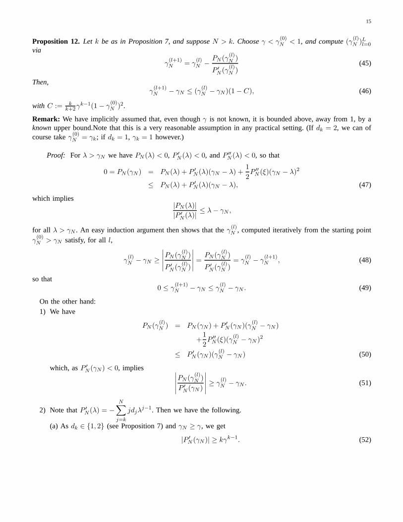
Fig. 10. The worst case error|γ − γN,I | for I = 2, 5, 10, 20, among 100 numerical experiments conducted in each case.

different sets of(xi, yi) pairs. Figure 10 shows the worst case approximation error,maxℓ |γ− γ(ℓ)N,I |, versusN

in each case(I = 2, 3, 5, 10, 20). Here γ(ℓ)N,I is the approximation obtained as above from theℓth experiment

(ℓ = 1, . . . , 100). We observe that the worst case error can be very large whenI is small, i.e., when we usea small number of(x, y) pairs (although in individual examples, one can have very good estimates as seenin Figure 9a). On the other hand, using a large number of(x, y) pairs makes the estimates significantly morereliable: we observe that the worst case error decreases exponentially fast asN increases.

Remark: Note that robustness remark 4) above has to be adapted in thiscase:γ would no longer be allowed tovary from one sampling interval to the next, since we would most likely obtain our different pairs from consecutivesamples. Some change ofγ would still be allowed without hurting the algorithm if it were sufficiently slow.

A different approach to determiningγ approximately from encoded sequences(bn) and (cn) is proposed in thenext subsection.

B. An alternative to exhaustive search

In this section, we present a fast algorithm to estimateγ using the sequencesb := Eµγ,δ(x) andc := Eµ

γ,δ(1− x)

wherex ∈ (0, 1) andEµγ,δ is defined as before. First, we defined := b + c, and rewrite (16), the constraint of the

main lemma, as0 ≤ PN (γ) ≤ 2CγN (44)

wherePN (λ) := 1 −∑N

j=1 djλj andN ≥ k = minj : j ∈ N anddj 6= 0. We then have the following.

Proposition 11. Let k be as above. ForN ≥ k, PN has exactly one rootγN in [γ, 1]. Moreover,γN satisfies|γ − γN | ≤ C ′γN whereC ′ is as defined in Lemma 4.

Proof: First, note thatPk(λ) = 1 − dkλk has a root atγk := (1/dk)1/k which satisfies0 < γ ≤ γk ≤ 1.

(Recall that, by Proposition 7,k cannot be arbitrarily large.) Moreover, forN ≥ k, PN (λ) ≤ Pk(λ) for all λ > 0(since eachdj is non-negative). Thus,PN (γk) ≤ 0 for all N ≥ k.

On the other hand, for any positive integerN , we havePN (γ) ≥ 1 −∑

∞

j=1 djγj = 0. SincePN is continuous

on [γ, γk], by the intermediate value theoremPn has a root in[γ, γk] ⊆ [γ, 1]. Also, sincePN is strictly decreasingfor N ≥ k, this root is the only root ofPN in [γ, 1]; we denote it byγN . Finally, Lemma 4 implies that|γ−γN | ≤C ′γN .

Proposition 11 shows that if we can approximateγN , the root ofPN in [γ, 1], by γN with a precision ofO(γN ),then |γ − γN | will also be of orderγN . SincePN is a ’nice’ polynomial in that it is strictly decreasing on[0, 1]with a strictly decreasing derivative, we can computeγN with an arbitrary precision using Newton’s method. As amatter of fact,

15

Proposition 12. Let k be as in Proposition 7, and supposeN > k. Chooseγ < γ(0)N < 1, and compute(γ(l)

N )Ll=0via

γ(l+1)N = γ

(l)N −

PN (γ(l)N )

P ′

N (γ(l)N )

(45)

Then,γ

(l+1)N − γN ≤ (γ

(l)N − γN )(1 − C), (46)

with C := kk+2γk−1(1 − γ

(0)N )2.

Remark: We have implicitly assumed that, even thoughγ is not known, it is bounded above, away from 1, by aknownupper bound.Note that this is a very reasonable assumption in any practical setting. (Ifdk = 2, we can ofcourse takeγ(0)

N = γk; if dk = 1, γk = 1 however.)

Proof: For λ > γN we havePN (λ) < 0, P ′

N (λ) < 0, andP ′′

N (λ) < 0, so that

0 = PN (γN ) = PN (λ) + P ′

N (λ)(γN − λ) +1

2P ′′

N (ξ)(γN − λ)2

≤ PN (λ) + P ′

N (λ)(γN − λ), (47)

which implies|PN (λ)|

|P ′

N (λ)|≤ λ − γN ,

for all λ > γN . An easy induction argument then shows that theγ(l)N , computed iteratively from the starting point

γ(0)N > γN satisfy, for all l,

γ(l)N − γN ≥

∣

∣

∣

∣

∣

PN (γ(l)N )

P ′

N (γ(l)N )

∣

∣

∣

∣

∣

=PN (γ

(l)N )

P ′

N (γ(l)N )

= γ(l)N − γ

(l+1)N , (48)

so that0 ≤ γ

(l+1)N − γN ≤ γ

(l)N − γN . (49)

On the other hand:

1) We have

PN (γ(l)N ) = PN (γN ) + P ′

N (γN )(γ(l)N − γN )

+1

2P ′′

N (ξ)(γ(l)N − γN )2

≤ P ′

N (γN )(γ(l)N − γN ) (50)

which, asP ′

N (γN ) < 0, implies∣

∣

∣

∣

∣

PN (γ(l)N )

P ′

N (γN )

∣

∣

∣

∣

∣

≥ γ(l)N − γN . (51)

2) Note thatP ′

N (λ) = −

N∑

j=k

jdjλj−1. Then we have the following.

(a) As dk ∈ 1, 2 (see Proposition 7) andγN ≥ γ, we get

|P ′

N (γN )| ≥ kγk−1. (52)

16

(b) Noting thatdj ∈ 0, 1, 2 for all j, we obtain

|P ′

N (γ(l)N )| ≤ 2

N∑

j=k

jλj−1 ≤ 2∞∑

j=k

jλj−1

= 2d

dλ(λk

∞∑

j=0

λj)

= 2λk−1 k(1 − λ) + 1

(1 − λ)2

for all 1 > λ ≥ γ(l)N . In particular, as1 > γ

(0)N ≥ γ

(l)N > 1

2 , we get

|P ′

N (γ(l)N )| ≤ 2

12k + 1

(1 − γ(0)N )2

(53)

Combining (51), (52), and (53), we conclude∣

∣

∣

∣

∣

PN (γ(l)N )

P ′

N (γ(l)N )

∣

∣

∣

∣

∣

=PN (γ

(l)N )

P ′

N (γ(l)N )

≥ C(γ(l)N − γN ), (54)

whereC := kk+2γk−1(1 − γ

(0)N )2. Then (45) implies

γ(l+1)N − γN = γ

(l)N − γN −

PN (γ(l)N )

P ′

N (γ(l)N )

≤ (γ(l)N − γN )(1 − C). (55)

Corollary 13. Let γN , γ(l)N , andC be as in Proposition 12. Then

γ(l)N − γN ≤ (1 − C)l(γ

(0)N − γN ). (56)

Therefore, forl ≥ 1log(1−C)(N log γ + log(γ

(0)N − γN )−1), we have

0 ≤ γ(l)N − γN ≤ γN . (57)

Remark: Corollary 13 shows that Newton’s method will compute an approximation with the desired precisionafter O(N) iterations. In practice, however, we observe that the convergence is much faster. Figure 11 summarizesthe outcome of a numerical experiment we conducted: We chosex ∈ (0, 1) randomly, and computedγN byapproximating the root of the polynomialPN via Newton’s method with 10 iterations. We repeated this for100different x values. In Figure 11, we plot|γ − γN | versusN . As one observes from the figure, the estimates aresatisfactory. Moreover, the computation is much faster compared to exhaustive search.

The case of unknowna

Finally, we return to the case when the value ofa is unknown to the decoder. We define the polynomialPN,I asin point b) of Section IV-A, and try to approximateγ by finding a root in(0.5, 1). Recall that, our goal in definingPN,I was the expectation that it has a single root in[0.5, 1], and this root is located at approximately the rightvalue. Clearly, this is not guaranteed, however our numerical experiments suggest thatPN,I indeed satisfies thisexpectation whenI is large (e.g. 20 in our numerical examples outlined in pointb) of Section IV-A. Also, notethatPN,I satisfies the constraint (43) at any of its roots. So, computing its root(s) shall not give us any estimate ofγ that is worse off than the estimate that we would have obtained via exhaustive search using the constraint (43).

17

0 20 40 60 80 10010

−20

10−15

10−10

10−5

100

N

|γ−γ N

|~

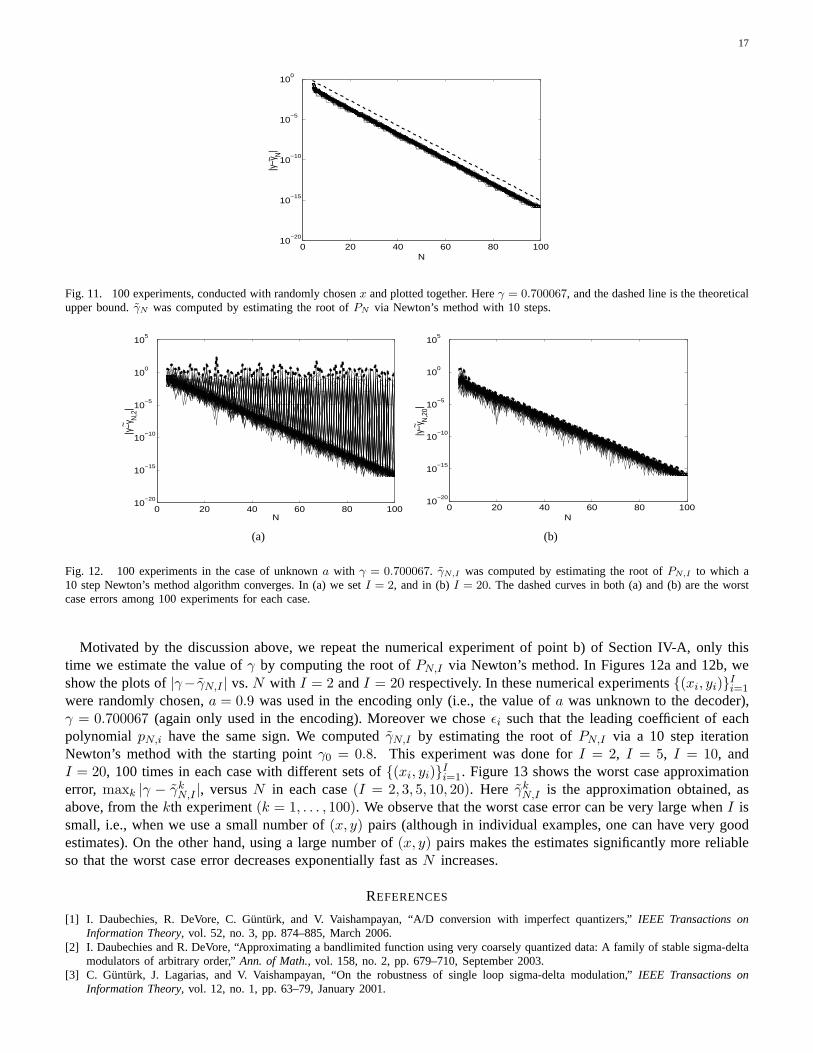
Fig. 11. 100 experiments, conducted with randomly chosenx and plotted together. Hereγ = 0.700067, and the dashed line is the theoreticalupper bound.γN was computed by estimating the root ofPN via Newton’s method with 10 steps.

0 20 40 60 80 10010

−20

10−15

10−10

10−5

100

105

N

|γ−γ N

,2|

~

(a)

0 20 40 60 80 10010

−20

10−15

10−10

10−5

100

105

N

|γ−γ N

,20|

~

(b)

Fig. 12. 100 experiments in the case of unknowna with γ = 0.700067. γN,I was computed by estimating the root ofPN,I to which a10 step Newton’s method algorithm converges. In (a) we setI = 2, and in (b)I = 20. The dashed curves in both (a) and (b) are the worstcase errors among 100 experiments for each case.

Motivated by the discussion above, we repeat the numerical experiment of point b) of Section IV-A, only thistime we estimate the value ofγ by computing the root ofPN,I via Newton’s method. In Figures 12a and 12b, weshow the plots of|γ− γN,I | vs.N with I = 2 andI = 20 respectively. In these numerical experiments(xi, yi)

Ii=1

were randomly chosen,a = 0.9 was used in the encoding only (i.e., the value ofa was unknown to the decoder),γ = 0.700067 (again only used in the encoding). Moreover we choseǫi such that the leading coefficient of eachpolynomial pN,i have the same sign. We computedγN,I by estimating the root ofPN,I via a 10 step iterationNewton’s method with the starting pointγ0 = 0.8. This experiment was done forI = 2, I = 5, I = 10, andI = 20, 100 times in each case with different sets of(xi, yi)

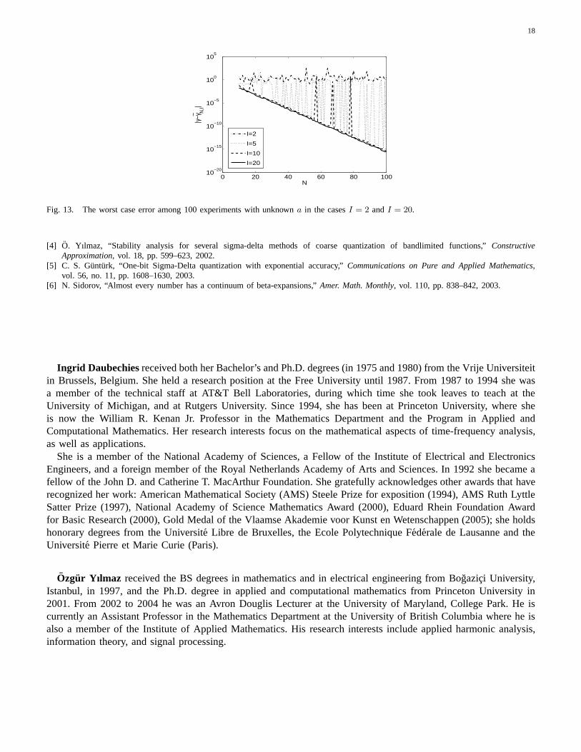
Ii=1. Figure 13 shows the worst case approximation

error, maxk |γ − γkN,I |, versusN in each case(I = 2, 3, 5, 10, 20). Here γk

N,I is the approximation obtained, asabove, from thekth experiment(k = 1, . . . , 100). We observe that the worst case error can be very large whenI issmall, i.e., when we use a small number of(x, y) pairs (although in individual examples, one can have very goodestimates). On the other hand, using a large number of(x, y) pairs makes the estimates significantly more reliableso that the worst case error decreases exponentially fast asN increases.

REFERENCES

[1] I. Daubechies, R. DeVore, C. Gunturk, and V. Vaishampayan, “A/D conversion with imperfect quantizers,”IEEE Transactions onInformation Theory, vol. 52, no. 3, pp. 874–885, March 2006.

[2] I. Daubechies and R. DeVore, “Approximating a bandlimited function using very coarsely quantized data: A family of stable sigma-deltamodulators of arbitrary order,”Ann. of Math., vol. 158, no. 2, pp. 679–710, September 2003.

[3] C. Gunturk, J. Lagarias, and V. Vaishampayan, “On the robustness of single loop sigma-delta modulation,”IEEE Transactions onInformation Theory, vol. 12, no. 1, pp. 63–79, January 2001.

18

0 20 40 60 80 10010

−20

10−15

10−10

10−5

100

105

N

|γ−γ N

,I|~

I=2

I=5

I=10

I=20

Fig. 13. The worst case error among 100 experiments with unknown a in the casesI = 2 andI = 20.

[4] O. Yılmaz, “Stability analysis for several sigma-delta methods of coarse quantization of bandlimited functions,”ConstructiveApproximation, vol. 18, pp. 599–623, 2002.

[5] C. S. Gunturk, “One-bit Sigma-Delta quantization with exponential accuracy,”Communications on Pure and Applied Mathematics,vol. 56, no. 11, pp. 1608–1630, 2003.

[6] N. Sidorov, “Almost every number has a continuum of beta-expansions,”Amer. Math. Monthly, vol. 110, pp. 838–842, 2003.

Ingrid Daubechiesreceived both her Bachelor’s and Ph.D. degrees (in 1975 and 1980) from the Vrije Universiteitin Brussels, Belgium. She held a research position at the Free University until 1987. From 1987 to 1994 she wasa member of the technical staff at AT&T Bell Laboratories, during which time she took leaves to teach at theUniversity of Michigan, and at Rutgers University. Since 1994, she has been at Princeton University, where sheis now the William R. Kenan Jr. Professor in the Mathematics Department and the Program in Applied andComputational Mathematics. Her research interests focus on the mathematical aspects of time-frequency analysis,as well as applications.

She is a member of the National Academy of Sciences, a Fellow of the Institute of Electrical and ElectronicsEngineers, and a foreign member of the Royal Netherlands Academy of Arts and Sciences. In 1992 she became afellow of the John D. and Catherine T. MacArthur Foundation.She gratefully acknowledges other awards that haverecognized her work: American Mathematical Society (AMS) Steele Prize for exposition (1994), AMS Ruth LyttleSatter Prize (1997), National Academy of Science Mathematics Award (2000), Eduard Rhein Foundation Awardfor Basic Research (2000), Gold Medal of the Vlaamse Akademie voor Kunst en Wetenschappen (2005); she holdshonorary degrees from the Universite Libre de Bruxelles, the Ecole Polytechnique Federale de Lausanne and theUniversite Pierre et Marie Curie (Paris).

Ozgur Yılmaz received the BS degrees in mathematics and in electrical engineering from Bogazici University,Istanbul, in 1997, and the Ph.D. degree in applied and computational mathematics from Princeton University in2001. From 2002 to 2004 he was an Avron Douglis Lecturer at theUniversity of Maryland, College Park. He iscurrently an Assistant Professor in the Mathematics Department at the University of British Columbia where he isalso a member of the Institute of Applied Mathematics. His research interests include applied harmonic analysis,information theory, and signal processing.