1. Report No. 2. Government Accession No. SWUTC/13 ... knowledge of speed and headway distributions is essential in microscopic traffic flow studies because speed and headway are both

1. Report No. SWUTC/13/600451-00020-1

2. Government Accession No.

3. Recipient's Catalog No.

4. Title and Subtitle A MULTIVARIATE ANALYSIS OF FREEWAY SPEED AND HEADWAY DATA

5. Report Date December 2013 6. Performing Organization Code

7. Author(s) Yajie Zou

8. Performing Organization Report No. Report 600451-00020-1

9. Performing Organization Name and Address Texas A&M Transportation Institute The Texas A&M University System College Station, Texas 77843-3135

10. Work Unit No. (TRAIS) 11. Contract or Grant No. DTRT 12-G-UTC06

12. Sponsoring Agency Name and Address Southwest Region University Transportation Center Texas A&M Transportation Institute The Texas A&M University System College Station, Texas 77843-3135

13. Type of Report and Period Covered 14. Sponsoring Agency Code

15. Supplementary Notes Partly supported by a grant from the U.S. Department of Transportation University Transportation Centers Program. 16. Abstract

The knowledge of speed and headway distributions is essential in microscopic traffic flow studies because speed and headway are both fundamental microscopic characteristics of traffic flow. For microscopic simulation models, one key process is the generation of entry vehicle speeds and vehicle arrival times. It is helpful to find desirable mathematical distributions to model individual speed and headway values, because the individual vehicle speed and arrival time in microscopic simulations are usually generated based on some form of mathematical models. Traditionally, distributions for speed and headway are investigated separately and independent of each other. However, this traditional approach ignores the possible dependence between speed and headway. To address this issue, the research presents a methodology to construct bivariate distributions to describe the characteristics of speed and headway. Based on the investigation of freeway speed and headway data measured from the loop detector data on IH-35 in Austin, it is shown that there exists a weak dependence between speed and headway.

The research first proposes skew-t mixture models to capture the heterogeneity in speed distribution. Finite mixture of skew-t distributions can significantly improve the goodness of fit of speed data. To develop a bivariate distribution to capture the dependence and describe the characteristics of speed and headway, this study proposes a Farlie-Gumbel-Morgenstern (FGM) approach to construct a bivariate distribution to simultaneously describe the characteristics of speed and headway. The bivariate model can provide a satisfactory fit to the multimodal speed and headway distribution. Overall, the proposed methodologies in this research can be used to generate more accurate vehicle speeds and vehicle arrival times by considering their dependence on each other when developing microscopic traffic simulation models.

17. Key Words Speed, headway, correlation, heterogeneity

18. Distribution Statement No restrictions. This document is available to the public through NTIS: National Technical Information Service 5285 Port Royal Road Springfield, Virginia 22161

19. Security Classif.(of this report) Unclassified

20. Security Classif.(of this page) Unclassified

21. No. of Pages 70

22. Price

Form DOT F 1700.7 (8-72) Reproduction of completed page authorized

A MULTIVARIATE ANALYSIS OF FREEWAY SPEED

AND HEADWAY DATA

By

Yajie Zou

Research assistant

Texas A&M Transportation Institute

December, 2013

i

DISCLAIMER

The contents of this report reflect the views of the author, who is responsible for the facts and the

accuracy of the information presented herein. This document is disseminated under the

sponsorship of the Department of Transportation, University Transportation Centers Program in

the interest of information exchange. The U.S. Government assumes no liability for the contents

or use thereof.

ACKNOWLEDGEMENT

The author recognizes that support for this dissertation was provided by a grant from the U.S.

Department of Transportation, University Transportation Centers Program to the Southwest

Region University Transportation Center.

ABSTRACT

The knowledge of speed and head way distributions is essent ial in m icroscopic traffic

flow studies because speed an d headway are both fundamental microscopic

characteristics of traffic flow. For microscopic simulation models, one key process is the

generation of entry vehicle speeds and vehicle arrival times. It is helpful to find desirable

mathematical distributions to m odel individual speed and headway values, because the

individual vehicle speed and arrival tim e in microscopic simulations are usu ally

generated based on som e form of mathematical models. Traditionally, distributions for

speed and headway are investigated separately and independent of each other. However,

this traditional approach ignores the possible dependence between speed and headway.

To address this issue, the research pr esents a m ethodology to construct bivariate

distributions to describe the characteri stics of speed and headway. Based on the

investigation of freeway speed and headway da ta measured from the loop detector data

on IH-35 in Austin, it is shown that there exists a weak dependence betw een speed and

headway.

The research first proposes skew-t m ixture models to capture the he terogeneity in speed

distribution. Finite m ixture of skew-t distributions can significantly im prove the

goodness of fit of speed data. To develop a bivariate distribut ion to capture the

dependence and describe the characteristics of speed and headway, this study proposes a

ii

Farlie-Gumbel-Morgenstern (FGM) approach to construct a bivariate distribution to

simultaneously describe the characteristics of speed and headway. The bivariate m odel

can provide a satisfactory fit to the multim odal speed and headway distribution. Overall,

the proposed m ethodologies in th is research can be used to generate m ore accurate

vehicle speeds and veh icle arrival times by considering th eir dependence on each other

when developing microscopic traffic simulation models.

iii

TABLE OF CONTENTS

Page

ABSTRACT ...................................................................................................................... II

TABLE OF CONTENTS ................................................................................................. IV

LIST OF FIGURES .......................................................................................................... VI

LIST OF TABLES ......................................................................................................... VII

CHAPTER I INTRODUCTION ....................................................................................... 1

1.1 Statement of the Problem ......................................................................................... 2 1.2 Research Objectives ................................................................................................. 3 1.3 Outline of the Research ............................................................................................ 4

CHAPTER II LITERATURE REVIEW ............................................................................ 6

2.1 Introduction .............................................................................................................. 6 2.2 Speed Distributions .................................................................................................. 6 2.3 Headway Distributions ............................................................................................. 7 2.4 Dependence between Speed and Headway .............................................................. 8 2.5 Summary .................................................................................................................. 8

CHAPTER III DATA INTRODUCTION AND PRELIMINARY ANALYSIS ............. 10

3.1 Introduction ............................................................................................................ 10 3.2 Data Description ..................................................................................................... 10 3.3 Preliminary Analysis .............................................................................................. 11 3.4 Summary ................................................................................................................ 18

CHAPTER IV METHODOLOGY I: MIXTURE MODELING OF FREEWAY SPEED DATA .................................................................................................................. 19

4.1 Introduction ............................................................................................................ 19 4.2 Finite Mixture Models ............................................................................................ 19 4.3 Model Estimation Method ...................................................................................... 22 4.4 Modeling Results ................................................................................................... 23 4.5 Summary ................................................................................................................ 33

iv

CHAPTER V METHODOLOGY II: MULTIVARIATE MIXTURE MODELING OF FREEWAY SPEED AND HEADWAY DATA ........................................................ 34

5.1 Introduction ............................................................................................................ 34 5.2 Methodology .......................................................................................................... 34 5.3 Results and discussions .......................................................................................... 41 5.4 Conclusions ............................................................................................................ 55

CHAPTER VI SUMMARY AND CONCLUSIONS ...................................................... 56

6.1 Summary ................................................................................................................ 56 6.2 Conclusions ............................................................................................................ 56 6.3 Future Research ...................................................................................................... 57

REFERENCES ................................................................................................................. 59

v

LIST OF FIGURES

Page

Figure 3.1 (a) speed scatter plots by time of day; (b) headway scatter plots by time of day; (c) vehicle length scatter plots by time of day; (d) hourly percentage of long vehicles by time of day. ............................................................................ 12

Figure 3.2 Scatter plot of speed and headway for peak period (T1). ............................... 18

Figure 4.1 The fitted mixture model for 2-component skew-t distribution. .................... 32

Figure 4.2 The mixture model for 4-component normal distribution. ............................. 33

Figure 5.1 24-hour speed and headway histograms (a) speed (b) headway. .................... 43

Figure 5.2 Bivariate speed and headway histogram and fitted distribution: (a) bivariate speed and headway histogram; (b) fitted bivariate distribution. ........ 52

vi

vii

LIST OF TABLES

Page Table 3.1 Summary statistics of speed and headway for different time periods .............. 15

Table 4.1 Computed AIC, BIC and ICL values for three mixture models ...................... 26

Table 4.2 The K-S test results for three mixture models ................................................. 28

Table 4.3 Parameter estimation results for the Skew-t mixture distribution .................... 30

Table 5.1 Parameter Estimation Results, R2 and RMSE Values for Speed Models ........ 42

Table 5.2 Parameter Estimation Results, R2 and RMSE Values for Headway Models ... 44

Table 5.3 Maximum Correlation Coefficients for Each Marginal Distribution ............... 45

Table 5.4 Summary Statistics of Headway for Each Speed Group .................................. 46

Table 5.5 Seemingly Unrelated Regression Model of Individual Vehicle Speed ........... 49

Table 5.6 Seemingly Unrelated Regression Model of Individual Vehicle Headway ..... 50

Table 5.7 R2 and RMSE Values for Bivariate Distributions ............................................ 51

CHAPTER I

INTRODUCTION

Speed is a funda mental measure of traffi c performance of a highway system (May,

1990). Most analytical and sim ulation models of traffic either produce speed as an

output or use speed as an input for travel ti me, delay, and level of service determ ination

(Park et al., 2010). It is desi rable to find an appropriate mathematical distribution to

describe the measured speeds, because in some microscopic simulations the individual

vehicle speed needs to be de termined according to some form of mathematical model

during vehicle generation (Park et al., 2010).

Headway is an important flow characteristic and headway distribut ion has applications

in capacity estim ation, driver behavior st udies and safety analysis (May, 1990). The

distribution of headway determ ines the re quirement and t he opportunity for passing,

merging, and crossing (May, 1990). The headway distribution under capacity-flow

conditions is also a primarily factor in determining the capacity of systems. Moreover, a

key component in m any microscopic simulation models is to gene rate entry vehicle

headway in the sim ulation process. To generate accura te vehicle arrival tim es to the

simulated network, it is necessary to use appropriate mathematical distributions to model

headway.

1

As described above, th e knowledge of speed and headway is necessary because these

variables are funda mental measures of tr affic performance of a hi ghway system.

Therefore, developing reliable and innovative analytical techniques for analyzing these

variables is very im portant. The primary goal of this research is to develop som e new

methodologies for the analysis of microscopic freeway speed and headway data.

1.1 Statement of the Problem

This research consists of two parts. The firs t part concerns the heterogeneity problem i n

freeway vehicle speed data. If the characteristics of speed data are homogeneous, speed

can be generally m odeled by normal, log-normal and gamma distributions. However, if

the speed data exhibit excess skewness and bimodality (or h eterogeneity), unimodal

distribution function does not give a satisfactory fit. Thus, the mixture model (composite

model) has been considered by May (1990) for traffic stream that consists of two classes

of vehicles or drivers. So far, the mixture models used in previous studies to fit bimodal

distribution of speed data c onsidered normal density as the specified com ponent;

therefore, it is useful to investigate other types of com ponent density for the finite

mixture model.

The second parts concern the dependence between freeway speed and headway data.

Traditionally, the dependence between speed and headway is ignored in the m icroscopic

simulation models. As a result, th e same headway distribution m ay be assum ed for

different speed levels and this assu mption neglects the pos sible variability of headway

2

distribution across speed values. Moreove r, a num ber of developed m icroscopic

simulation models generate vehicle speeds and vehicle arrival tim es as independent

inputs to the sim ulation process. Up to date , only a few st udies have been directed at

exploring the dependence between speed and headway. Considering the potential

dependence between speed and headway, it is us eful to construct bi variate distribution

models to describ e the characteris tics of speed and headway. Compared with o ne

dimensional statistical models representi ng speed or headway separately, bivariate

distributions have the advantage that the possible correlation between speed and

headway is taken in to consideration. Given th is advantage, it is neces sary to cons truct

bivariate distributions to improve the accuracy or validity of microscopic simulation

models.

1.2 Research Objectives

The primary goal of this research is to develop new m ethodologies for analyzing the

characteristics of speed and headway. To acco mplish this goal, following objectives are

planned to be addressed in this research.

1. To address the heterogeneity problem in freeway vehicle sp eed data, we apply

skew-normal and skew -t mixture models to capture excess skewness, kurtos is and

bimodality present in speed distribution. Sk ew-normal and skew-t distributions are

known for their flexibility, allowing for hea vy tails, high degree of kurtosis and

asymmetry. To investigate the applicability of mixture models with skew-norm al and

3

skew-t component density, we fit a 24-hour speed data collected on IH-35 using skew-

normal and skew-t mixture models with the Expectation Maximization type algorithm.

2. To construct bivariate distribution of speed and headway, we exam ine the

dependence structure between th e two variables. Three correlation coefficients (i.e.,

Pearson correlation coefficient, Spearman’s rho and Kendall’s tau) are used to evaluate

the dependence between speed and headway.

3. To develop a bivariate di stribution for capturing the dependence and describing

the characteristics of speed an d headway simultaneously, the Farlie-Gumbel -

Morgenstern (FGM) approach is proposed.

1.3 Outline of the Research

The rest of this research is organized as follows:

Chapter II overviews various mathematical models that have been used for describing

speed and headway distributions. S ome studies that focused on the dependence between

speed and headway are also discussed.

Chapter III provides the charac teristics of the traffic dataset used throughout in the

research. A preliminary analysis is conducte d to investigate the dependence structure

between speed and headway.

4

Chapter IV applies skew-t mixture models to fit freeway sp eed data. This chapter shows

that finite mixture of skew-t distributions can significantly improve the goodness of fit of

speed data and better account for heterogeneity in the data.

Chapter V explores the applicability of the FGM approach to address the heterogeneity

problem in speed and headway data. This ch apter shows that the bivariate m odel can

provide a satisfactory fit to the speed and headway data.

Chapter VI summarizes the major results of in this research. General conclusions and

recommendations for future research are presented.

5

CHAPTER II

LITERATURE REVIEW

2.1 Introduction

This chapter first provides a review of mathematical models for speed and headway.

Specifically, different speed and headway dist ributions proposed in the past studies are

introduced. Then, we discuss som e research focused on the dependence between speed

and headway.

2.2 Speed Distributions

Previously, normal, log-normal and other form s of distribution have been used to fit

freeway speed data. L eong (1968) and McL ean (1979) proposed that speed data

approximately follow a norm al distribution when flow rate is light. Haight and Mosher

(1962) showed that the log-norm al distribution is proper for speed data. Gerlough and

Huber (1976) and Haight (1965) have used nor mal, log-normal and gamma distributions

to model vehicular speed. Compared with normal distribution, log-normal and gamma

distributions have the capacity to accommodate the rig ht skewness and elim inate

negative speed values generated by norm al distribution. If the speed data exhibit excess

skewness and bimodality, unimodal distribution function does not give a satisfactory fit;

thus, several researchers used the m ixture model to fit the distribution of speed. W hen

the traffic stream consists of two vehicle types, the com posite distribution has been

proposed by May (1990). He also suggested that the vehicle sp eeds for subpopulations

6

follow normal or lognormal distributions. Dey et al. (2006) introduced a new param eter,

spread ratio to predict the shape of the speed curve. He stated that the bim odal speed

distribution curve consists of a mixture of two-speed fractions, lower fraction and upper

fraction. Ko and Guensler (2005) did a si milar study by characterizing the speed data

with two different norm al components, one for congested and the other for non-

congested speeds. The congestion characteri stics can be identified based on the speed

distribution. Recently, Park et al. (2010) explored the distribution of 24-hour speed data

with a g-component norm al mixture model. Jun (2010) investigated traffic congestion

trends by speed patterns during holiday travel periods using the normal mixture model.

2.3 Headway Distributions

Many headway models have been proposed and these models can be classified into two

types: single distribution m odels and m ixed models. For single distribution m odels,

exponential (Cowan, 1975), norm al, gamma, lognormal and l og-logistic distributions

(Yin et al., 2009) have been studied to m odel headway. The representatives of m ixed

models are Cowan M3 model (Luttine n, 1999), M4 m odel (Hoogendoorn and Bovy,

1998), the generalized queuing model and the semi-Poisson model (Wasielewski, 1979).

Zhang et al. (2007) perfor med a c omprehensive study of the perform ance of typical

headway models using the headway data recorded from general-purpose lanes.

7

2.4 Dependence between Speed and Headway

There have been som e studies that focu sed on the dependence between speed and

headway. Luttinen (1992) found out that speed limit and road category have a

considerable effect on the sta tistical properties of vehicle h eadways. WINSUM and

Heino (1996) investigated the time headway and braking response during car-following.

Taieb-Maimon and Shinar (2001) conducted a study to investigate drivers’ following

headways in car -following situation and th e results showed that drivers adjusted the

distance headways in relation to speed. Dey and Chandra (2009) proposed two statistical

distributions for m odeling the gap and h eadway in the steady car-following state.

Brackstone et al. (2009) found th at there is a limited depe ndence of following headway

on speed and the m ost successful relationship fit of headway and speed is an inverse

relationship. Yin et al. (2009) also studied the dependence of headway distributions on

the traffic condition (speed pattern) and concluded that different headway models should

be used for distinct traffic conditions (speed patterns).

2.5 Summary

From the above discussion, th ere are several current issu es existing in m odeling the

speed and headway data. First, when modeling multimodal distribution of speed data, the

mixture models used in previous studies ex tensively considered normal density as the

specified component; therefore, other type s of com ponent density were not fully

investigated. Second, considering the possi ble dependence between speed and headway,

8

there were very few studies focusing on cons tructing bivariate distribution m odels to

describe speed and headway simultaneously.

9

CHAPTER III

DATA INTRODUCTION AND PRELIMINARY ANALYSIS

3.1 Introduction

As discussed in Chap ter I, the main objective of this r esearch is to develop new

methodologies for analyzing the characteristics of freeway speed and headway data. The

traffic data analyzed in this research are the microscopic traffic variables (i.e., individual

speed and headway observations) measured from the loop detector data. The study site is

on IH-35 in Austin, Texas. This c hapter introduces the c haracteristics of the tra ffic

dataset which is used throughout in the resear ch. A preliminary analysis is conducted to

investigate the dependence structure between observed speed and headway data.

3.2 Data Description

The dataset was collected at a location on IH -35. IH-35 has four lanes in the southbound

direction and the free flow speed is 60 m ile/hour (or 96.56 kilometer/hour) for all types

of vehicles. Due to the heavy traffic dem and and a large volum e of heavy vehicles, the

data collection site is typi cally congested during the m orning and afternoon peak hours.

The detector records vehicle arrival time, presence time, speed, length, and classification

for each individual vehicle (Ye et al., 2006). This dataset was analyzed in some previous

studies (Ye and Zhang, 2009). The data have 27920 vehicles with recorded speed values,

arrival times and vehicle lengths in a 24-hour period (from 00:00 to 24:00, December 11,

2004), including 24011 (86%) passenger vehicl es and 3909 (14%) heavy vehicles. For

10

this dataset, the headwa y value be tween two consecutive vehicles is the elaps ed time

between the arrivals of a pair of vehicles. Th e arrival times were recorded in second (s);

the observed speeds w ere recorded in m eter/second; and the vehicle lengths were

recorded in meter (m). To compare the result of this work with som e previous studies,

we convert the m eter/second to kilom eter/hour (kph). W e also assume that 24-hour

period (T) consists of two time periods: the p eak time period (T1) which contains two

sub-periods 07:10-08:20 and 15:22-19:33; whil e the off peak period (T2) includes two

sub-periods 08:20-15:22 and 19:33-07:10.

3.3 Preliminary Analysis

Figure 3.1 (a), (b) and (c) display the scatte r plots of speed, headway and vehicle length

by time of day for each tim e period. Because of large samples in th e dataset, sem i-

transparent points are used to alleviate som e of the over-plotting in Figure 3.1. Figure

3.1 (c) indicates that the observed vehicles seem to consist of two sub-populations: one

at about 5 m eters, representing passenger ve hicles, and the other at about 22 m eters,

representing trucks and buses. Previously, Zhang et al. (2008) estimated large truck

volume using loop detector data collected from IH-35, and they classified vehicles into

two categories: short vehicles (smaller than 12.2 m (40 feet)) and long vehicles (larger

than or equal to 12.2 m (40 feet)). In orde r to see the changing pattern of vehicle

composition over the tim e, we calculate the hour ly percentage of long vehicles (greater

than or equal to 12.2 m ), which is shown in Figure 3.1 (d). It can be observed that the

11

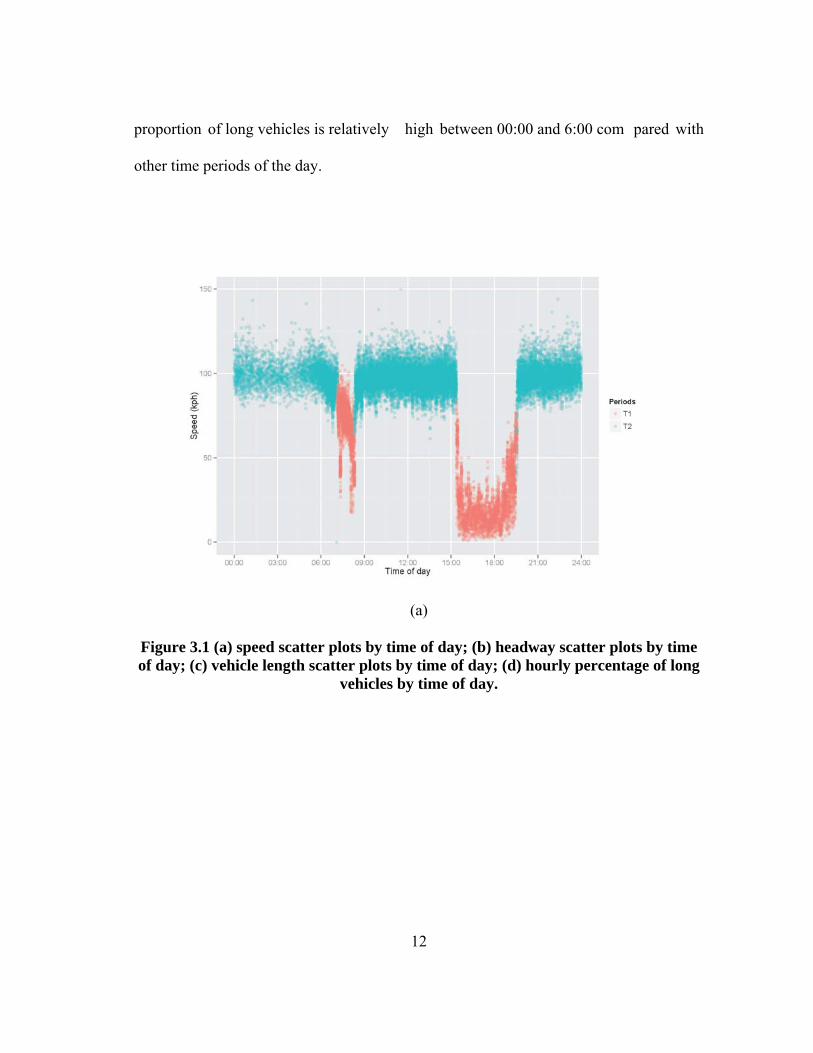
proportion of long vehicles is relatively high between 00:00 and 6:00 com pared with

other time periods of the day.

(a)

Figure 3.1 (a) speed scatter plots by time of day; (b) headway scatter plots by time of day; (c) vehicle length scatter plots by time of day; (d) hourly percentage of long

vehicles by time of day.

12

(b)

(c)

Figure 3.1 Continued

13

(d)

Figure 3.1 Continued

14

From Figure 3.1 (a), we can see that the speed data exhibit hetero geneity and the m ain

cause for this heterog eneity is different traffic flow conditions over the 2 4-hour period.

Since the characteristics of speed data are heterogeneous, the mixture models are used to

capture bimodality present in speed dist ribution. Then, we exam ine the correlation

between speed and headway. Since the 24-hour traffic data in the study consist of

distinct traffic flow conditions, it is useful to evaluate the dependence between vehicle

speed and headway under different traffic conditions. As discussed above, we divided

the 24-hour traffic data into two tim e periods (i.e., the peak period T1 and the off-peak

period T2) based on correspond ing traffic conditions. For each tim e period, three

correlation coefficients are used to evaluate the dependence. These three m easures of

dependence are Pearson correlation coeffi cient (PCC), Spearm an’s tau (SCC), and

Kendall’s pho (KCC). The summ ary statistics of speed and headway for different tim e

periods are given in Table 3.1.

Table 3.1 Summary statistics of speed and headway for different time periods

T (24 hours)

T1 (07:10-08:20 and

15:22-19:33)

T2 (08:20-15:22 and

19:33-07:10)

Speed Headway Speed Headway Speed Headway

Min. 0 0 a 1.01 0 0 0

1st Quantile 84.74 1 18.22 2 92.38 1

Median 94.57 2 37.76 2 97.09 2

Mean 85.3 3.1 42.71 3.15 97.24 3.08

3rd Quantile 100.4 3 68.57 4 101.95 3

Max. 149.69 76 104.72 48 149.69 76

Number of

vehicles 27919 6114 21805

PCC -0.054 -0.469 0.116

KCC 0.003 -0.488 0.135

SCC 0.011 -0.635 0.186

Note: a Headway values are less than 0.5s.

15

PCC measures the linear relationship between tw o continuous variables. It is defined as

the ratio of the covariance of the two variables to the product of their respective standard

deviations:

( , )PCCx y

Cov x yσ σ

= (3.1)

where xσ and yσ are the standard deviations of variables x and y.

SCC is a rank-based version of the PCC and it can be computed as:

1

2 2

1 1

( ( ) ( ))( ( ) ( ))SCC

( ( ) ( )) ( ( ) ( ))

n

i ii

n n

i ii i

rank x rank x rank y rank y

rank x rank x rank y rank y

=

= =

− −=

− −

∑

∑ ∑ (3.2)

where and ( )irank x ( )irank y are the ranks of the observation ix and iy in the sample.

Similar to SCC, KCC is designed to cap ture the asso ciation between two m easured

quantities. KCC quantifies th e discrepancy between the nu mber of concordant and

discordant pairs. Its estimate can be expressed as follows:

1 1sgn( )sgn( )

KCC= 1 ( 1)2

n n

i j i ji j

x x y y

n n

= =

− −

−

∑∑ (3.3)

where 1 if ( ) 0

sgn( ) 0 if ( ) 01 if ( ) 0

i j

i j i j

i j

x xx x x x

x x

⎧ − >⎪− = − =⎨⎪− −⎩ <

and 1 if ( ) 0

sgn( ) 0 if ( ) 01 if ( ) 0

i j

i j i j

i j

y yy y y y

y y

⎧ − >⎪− = −⎨⎪

=− − <⎩

.

16

Note that the PCC, KCC, and SCC are -0 .469, -0.488 and -0.635 between speed and

headway for peak perio d T1, suggesting a moderate inverse relationship between these

two traffic variables. Since speed and headway values in peak period T 1 were observed

under congested traffic conditi ons, it is reason able to con sider most of the headway

values in time period T1 as following headwa ys. From Figure 3.2, it is observed that

headway increases as speed decreases, and the relationship can be split into two regimes.

The time headway is approxim ately stable when speed is above 20 kph in the first

regime. In the second regim e when speed is b elow 20 kph, the tim e headway increases

significantly as sp eed decreases. The findings from Figure 3.2 are c onsistent with the

results reported in a study conducted by Brackstone et al. (2009 ). In their study, it is

shown that there is a lim ited dependence of following headway on speed: the m ost

successful relationship fit of headway and speed is an inverse relationship. Interestingly,

KCC is 0.135 between speed and headway fo r off-peak period T2, indicating a positive

dependence. This is reasonable because as h eadway values become larger during the off

peak period, fewer vehicles are on th e road and it is expected to see that vehicle speeds

increase accordingly.

17

Figure 3.2 Scatter plot of speed and headway for peak period (T1).

3.4 Summary

This chapter described the characteristics of traffic data collected on IH-35. As shown in

Figure 3.1 (a), the speed data are heterogeneous and to capture the bimodality present in

the speed distribution, Chapter IV proposes skew-t mixture models to fit freeway speed

data. Besides, the d ata analysis in dicates that the two m icroscopic traffic variables

(speed and headway) are correlated under di fferent traffic conditi ons and to construct

bivariate distribution of speed and headwa y, the FGM approach is p roposed in the

Chapter V.

18

CHAPTER IV

METHODOLOGY I: MIXTURE MODELING OF FREEWAY SPEED DATA1

4.1 Introduction

An appropriate mathematical distribution can help describing speed characteristics and is

also useful for developing and validating microscopic traffic simulation models. To

accommodate the hetero geneity in speed data , the m ixture models used in previo us

studies extensively considered normal density as the specified com ponent; therefore,

other types of com ponent density were not fully investigated. To capture ex cess

skewness, kurtosis and bimodality present in speed dis tribution, we propose sk ew-

normal and skew-t m ixture models to fit fr eeway speed data. This chapter shows that

finite mixture of skew-t distribution s can significantly im prove the goodness of fit of

speed data and better account for heterogeneity in the data.

4.2 Finite Mixture Models

In this chapter, it is assumed that the speed data are indepe ndent and identically

distributed (i.i.d.) realizations from a random variable which follows either a m ixture of

g-component normal, skew-normal or skew-t mixture model. The m ixture model is

19

1 Reprinted with perm ission from “ Use of skew-normal and skew-t distributions for mixture modeling of freeway speed da ta” by ZOU, Y. , & ZHANG, Y., 2011. Transportation Research Record, 2260, 67-75, Copyright [2011] by the Transportation Research Board.

widely used in m odeling bimodal speed dist ribution to account for the heterogeneity.

The normal, skew-normal and skew-t m ixture models are briefly introduced in this

section:

The normal mixture model for the vehicle sp eed has the following probability density

function:

2 2

1

( | , , ) ( | , )N

k k k k k kk

f x w w NL xξ σ ξ=

=∑ σ

(4.1)

22

22

( )1( | , ) exp( )22

kk k

kk

xNL x ξξ σσπσ

−= −

(4.2)

The expectation and variance of a normal distribution can be written as:

( ) kE x ξ= (4.3)

2( ) kVar x σ= (4.4)

where is the num ber of com ponents, is the weight of com ponent k , with

and ,

N

1 0>

kw

kw>1

1N

kk

w=

=∑ kξ is the location pa rameter, 2kσ is the sca le parameter, and

2 )k( | ,NL x kξ σ is the normal density function with mean kξ and variance 2kσ .

The skew-normal distribution was first developed by Azzalini (1985). The probability

density function for the skew-normal mixture model is given by:

20

2 2

1

( | , , , ) ( | , , )N

k k k k k k k kk

f x w w SN xξ σ λ ξ σ λ=

=∑

(4.5)

2 2( | , , ) k kk k k k

k k k

x xSN x ξ ξξ σ λ φ λσ σ σ

⎛ ⎞ ⎛− −= Φ⎜ ⎟ ⎜

⎝ ⎠ ⎝

⎞⎟⎠

(4.6)

The expectation and variance of a skew-normal distribution are given by

2( ) k kE x ξ σδπ

= + (4.7)

22 2( ) 1 kkVar x δσ

π⎛ ⎞

= −⎜ ⎟⎝ ⎠

(4.8)

where 21

kk

k

λδλ

=+

, kλ is the skewness parameter, ( )φ ⋅ and ( )Φ ⋅

2( | ,k k

are, the standard

normal density and cum ulative distribution function, and , )kxSN ξ σ λ

( | , )kx

is the skew-

normal density function. The m ean and variance of 2,k kSN ξ σ λ are given in

equations (4.7) and (4.8), respectively.

It can be shown that the excess kurtosis of a skew-normal distribution is limited to the

interval [0, 0.8692]. Late r, the skew-t distribu tion was introduced by Azzalini and

Capitanio (2003) to allow for a higher degree of kurto sis. The skew-t mixture model can

be written as follows:

2 2

1

( | , , , , ) ( | , , , )N

k k k k k k k kk

f y w v w ST y vξ σ λ ξ σ λ=

=∑

(4.9)

21

21 2

2 1( | , , , ) ( )k k k y k yk y

ST y t x T xxν ν

νξ σ λ ν λσ ν+

⎛ ⎞+= ⎜ ⎟⎜ ⎟+⎝ ⎠

(4.10)

where ν is the degrees o f freedom, ( ) /y kx y kξ σ= − , tν and Tν represent the stan dard

Student-t density and cum ulative function with ν degrees of fr eedom, and

2( | , , , )k k kST y ξ σ λ ν is the skew-t density function. Al so, it can be shown that the skew-t

distribution converges to a skew-normal distribution when ν →∝ (ν tends to infinity).

4.3 Model Estimation Method

There are various m ethods available for es timating a m ixture model. The m ethod of

moments was first used by Pearson in th e early days of mixture modeling. The

maximum likelihood estim ation with Expect ation Maximization (EM) algorithm and

Bayesian estimation become the most widely applied methods when large calculations

can be easily done by powerful computers. Assuming the num ber of com ponents is

known, Bayesian approach can be im plemented with data augm entation and Markov

Chain Monte Carlo (MCMC) estim ation procedure using Gibbs sam pling techniques

(Zou et al, 2012). However, one of the m ain drawbacks of MCMC pr ocedures is that

they are generally computationally de manding, and it can be diffic ult to diagnose

convergence (Zou et al, 2012). Furthermore, the label switching is another difficulty and

has to be addressed ex plicitly when using a Bayesian app roach to co nduct parameter

estimation and clustering (Frühwirth-Schnatter, 2006).

22

Since the label switching is of no con cern for m aximum likelihood estim ation, the

maximum likelihood method is adopted for estim ation of finite mixture of skew-normal

and skew-t distributions in this study. The EM algorithm was introduced by Dempster et

al. (1977) and there are two extensions of it: the Expectation/Conditional Maximization

Either (ECME) and the Expectation/Condi tional Maximization (ECM) algorithms.

Among the three algorithm s, the ECM algorith m converges more slowly than the EM

algorithm, but consumes less processing time in computer. The ECME algorithm has the

greatest speed of convergence as well as the least processing tim e; moreover, it

preserves the stability with monotone convergence. Thus, the ECME algorithm is chosen

for the estimation of the parameters here.

4.4 Modeling Results

We apply normal, skew-normal and skew-t mixture models with an increasing number

of components (g =2,…,6) to the 24-hour sp eed data described in Chapter III. The

ECME algorithm is coded and run until th e convergence maximum error 0.0000001 is

satisfied or until the m aximum number of it erations 3000 is reach ed. A common

problem with this m ethod is that the EM type algorithm may lead to a local m aximum

and one feasible solution to find the global m aximum is to try m any different initial

values. Therefore, the procedure described by Basso et al. (2010) is adopted to ensure

that initial values are not far from the real parameter values.

23

4.4.1 Determination of optimal model

To select th e most appropriate model from normal, skew-normal and skew-t m ixture

models, the Akaike Inform ation Criterion (A IC), the Bayesian Inform ation Criterion

(BIC), and the Integ rated Completed Likelihood Criterion (ICL) ar e computed for each

mixture model. AIC and BIC have the sam e form 2 nLL cγ− + , where LL is the log-

likelihood value, γ is the number of f ree parameters to be estim ated and is the

penalty term with a positive value.

nc

The value o f is defined depending on the select ed criterion. For AIC and BIC,

equals 2 and l respectively, where n is the number of observations. The ICL

criterion approximated from a BIC- like approximation is defined as

nc nc

)

og( )n

*2 log(LL nγ− + ,

where is the integrated log-likelihood. It is known that BIC is m ore conservative

than AIC. In the density estimation context, BIC is a reliable tool for comparing mixture

models. When choosing the form of the model, using BIC as the criterion usually results

in a good fit of data. If the finite m ixture model is correctly specifi ed, BIC is known to

be consistent. On the other hand, if the con cern of mixture modeling is cluster analysis,

ICL criterion is preferred over BIC when selecting the optimal number of components g,

because BIC may overestimate the number of components (

*LL

Biernacki et al., 2000 ). In

particular, BIC is likely to be imprecise in id entifying the correct size of the clusters

when component densities of m ixture model are not specified correctly. The ICL

24

criterion includes an additional entropy term which favors well-separated clusters

(Biernacki et al., 2000).

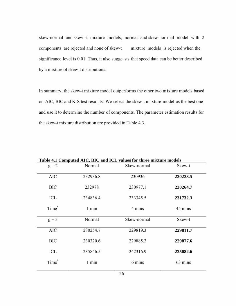
Bold values in Table 4.1 report the sm allest AIC, BIC a mong three m ixture models.

Smaller AIC and BIC values indicate a better overall fit. Based on the results, the skew-t

mixture model is selected as the best one for g = 2, 3, 5, 6. For g = 4, the skew-norm al

mixture model is slightly better than the skew-t mixture model in terms of AIC and BIC

values. Upon com parison of three m ixture models, we find that the skew-norm al and

skew-t mixture models both show a m uch better fitting result than the normal mixture

model; the skew-t m ixture model has the smallest AIC and BIC values except when g

equals 4. The computation times for each model are shown in Table 4.1. Compared with

the normal mixture model, the skew-normal mixture model can significantly improve the

goodness of fit of speed data while the increase in com putational effort is not

remarkable. Given this advantage, the skew -normal mixture model can be used as an

alternative to the skew-t mixture model if the computation time is limited. And the skew-

t mixture model can achieve the best fitting result at the cost of more computation time.

Another important criterion considered fo r model assessm ent is the Kol mogorov-

Smirnov’s (K-S) goodness of fit test ( Lin et al., 2007 ). We perfor med K-S tests to

validate the above three m ixture models. The statistics D and p-valu e for K-S tests are

summarized in Tab le 4.2. Note that in a K-S te st, given a sufficiently large sample, a

small and non-notable statistics D can be found to be statistically significant. For normal,

25

skew-normal and skew -t mixture models, normal and skew-nor mal model with 2

components are rejected and none of skew-t mixture models is rejected when the

significance level is 0.01. Thus, it also sugge sts that speed data can be better described

by a mixture of skew-t distributions.

In summary, the skew-t mixture model outperforms the other two mixture models based

on AIC, BIC and K-S test resu lts. We select the skew-t m ixture model as the best one

and use it to determ ine the number of components. The parameter estimation results for

the skew-t mixture distribution are provided in Table 4.3.

Table 4.1 Computed AIC, BIC and ICL values for three mixture models

26

g = 2 Normal Skew-normal Skew-t

AIC 232936.8 230936 230223.5

BIC 232978 230977.1 230264.7

ICL 234836.4 233345.5 231732.3

Time* 1 min 4 mins 45 mins


AIC 230254.7 229819.3 229811.7

BIC 230320.6 229885.2 229877.6

ICL 235846.5 242316.9 235082.6

Time* 1 min 6 mins 63 mins

Table 4.1 Continued


AIC 229921.4 229801.9 229802

BIC 230012 229892.5 229892.6

ICL 239894 256410.1 250663.8

Time* 4 mins 8 mins 363 mins


AIC 229836.3 229745 229740.6

BIC 229951.6 229860.4 229855.9

ICL 251178.7 247112.5 251844.7



AIC 229809.1 229786.7 229746

BIC 229949.2 229926.7 229886

ICL 257663.9 243317.1 245020.3


∗ These experiments were performed on a desktop with Core 2 Duo processor E8500 running at 3.16 GHz and 4 GB RAM.

27

Table 4.2 The K-S test results for three mixture models No. of components Normal Skew-normal Skew-t

D p-value D p-value D p-value

g = 2 0.0275 0.0000 0.0220 0.0000 0.0146 0.0109

g = 3 0.0117 0.04242 0.0074 0.4796 0.0074 0.4825

g = 4 0.009 0.2055 0.0072 0.5016 0.0071 0.5141

g = 5 0.007 0.5038 0.0069 0.5444 0.0070 0.5256

g = 6 0.0067 0.5583 0.0073 0.4894 0.0067 0.5764

4.4.2 Selecting the number of components

It is quite a challenge to de termine the optimal number of components in finite mixture

models. Currently, available methods include reversible jump MCMC and model choice

criteria. For skew-t mixture models, the implementation of reversible jump MCMC turns

out to be very com plicated and computation of marginal likelihoods remains an i ssue.

Thus, we adopted the m odel choice criteria. As mentioned before, AIC tends to select

too many components and BIC overrates the nu mber of components if the com ponent

densities are misspecified. ICL criterion seems to provide a reliable estimate of g for real

data (Biernacki et al., 2000 ). Thus, ICL values reported in Table 4.1 are used to

determine the optimal number of components. Based on ICL criterion, g = 2 is chosen

for the skew-t m ixture model. Previously, Park et al. (20 10) explored the da ta with a

normal mixture model and selected the optimal number of components g = 4. To provide

28

further insight into the pattern of m ixture, we f it the speed dis tribution with a 2-

component skew-t mixture model and a 4-component normal mixture model.

The mixture density as well as each component-wise density for the 2-component skew-t

and 4-component normal mixture distributions are displayed in Figure 4.1 and Figure

4.2, respectively. Based on the graphical vi sualization, both 2-component skew-t and 4-

component normal mixture models fit th e 24-hour speed distribution very well.

However, as shown in these figures, the bimodality of the speed distribution suggests the

presence of 2 different speed groups. One skew -t distribution can adequately capture the

skewness and kurtosis present in one cluster; by contrast , two normal m ixtures are

needed to accommodate the skewness and kurto sis of one speed group. It is observed in

Figure 4.1 that cluster 1 is composed of speed data from group 1 and cluster 2 consists of

speed data from group 2. Since group 1 and group 2 represent distinct traffic flow

characteristics, this verifies that traffic flow condition is the main cause for heterogeneity

in this 24-hour speed data. On the other hand, no clear interpretation can be m ade

regarding different flow conditions if a 4-component normal mixture model is used.

To summarize, th e skew-t m ixture model classified veh icle speed into 2 clu sters.

Component 1 (high speed cluster) includes vehicles in uncongested traffic condition and

a large portion of vehicles in transition flow condition. Component 2 (low speed cluster)

has a large variance and repres ents vehicles in congested traffic condition and a sm all

portion of vehicles in transition flow condition.

29

Table 4.3 Parameter estimation results for the Skew-t mixture distribution Component Parameters 1 2 3 4 5 6

g=2 ξ 101.71 6.96

2σ 79.01 491.72

λ -1.07 8.06

nu* 3.59 3.59

η 0.85 0.15

g=3 ξ 88.21 93.92 7.27

2σ 298.74 55.04 363.48

λ -1.08 0.72 6.09

nu* 9.33 9.33 9.33

η 0.14 0.73 0.13

g=4 ξ 78.36 93.66 7.23 99.78

2σ 254.36 85.60 375.22 90.90

λ -2.33 1.92 6.09 -1.52

nu* 15.05 15.05 15.05 15.05

η 0.07 0.39 0.13 0.41

30

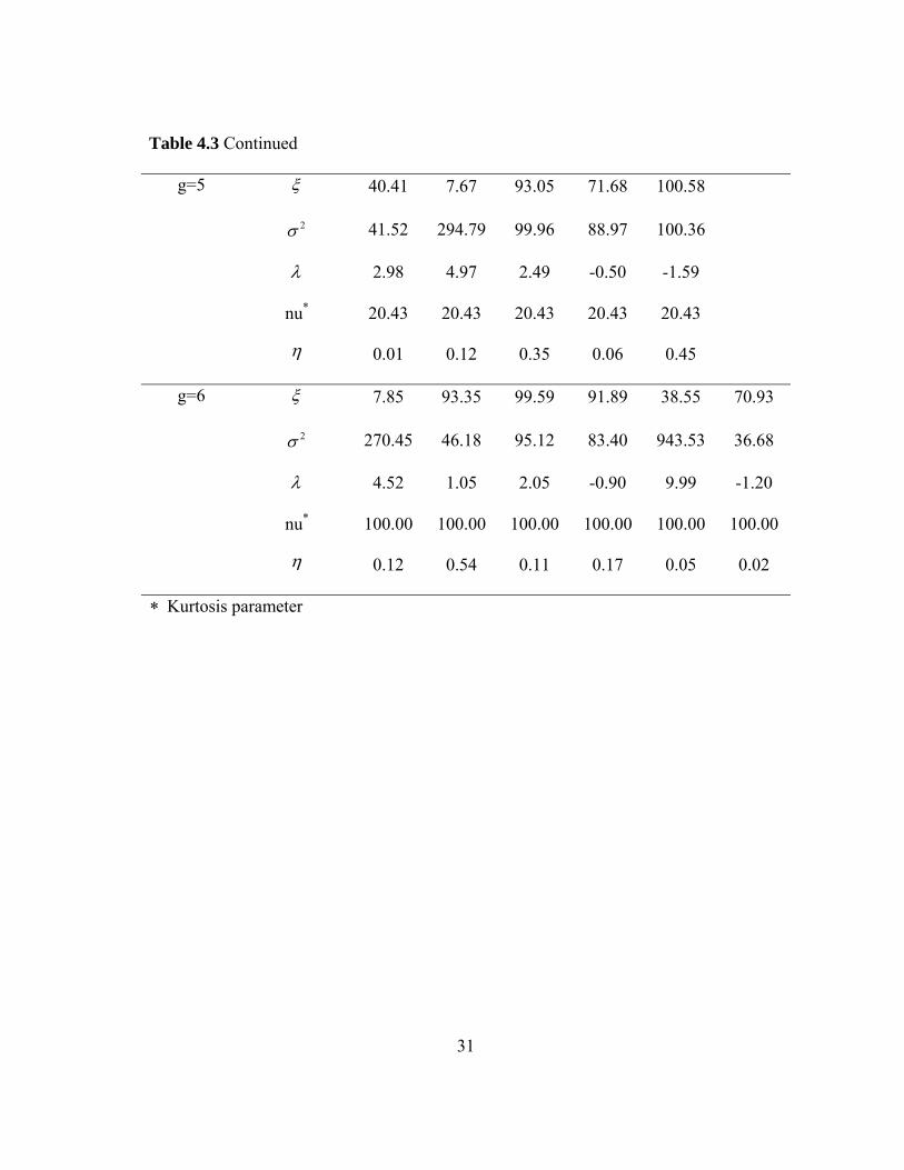
Table 4.3 Continued

g=5 ξ 40.41 7.67 93.05 71.68 100.58

2σ 41.52 294.79 99.96 88.97 100.36

λ 2.98 4.97 2.49 -0.50 -1.59

nu* 20.43 20.43 20.43 20.43 20.43

η 0.01 0.12 0.35 0.06 0.45

g=6 ξ 7.85 93.35 99.59 91.89 38.55 70.93

2σ 270.45 46.18 95.12 83.40 943.53 36.68

λ 4.52 1.05 2.05 -0.90 9.99 -1.20

nu* 100.00 100.00 100.00 100.00 100.00 100.00

η 0.12 0.54 0.11 0.17 0.05 0.02

∗ Kurtosis parameter

31

Speed (kph)

coun

t

0

500

1000

1500

2000

2500

0 20 40 60 80 100 120 140

Group

G1

G2

Figure 4.1 The fitted mixture model for 2-component skew-t distribution.

32

Speed (kph)

coun

t

0

500

1000

1500

2000

2500

0 20 40 60 80 100 120 140

Group

G1

G2

Figure 4.2 The mixture model for 4-component normal distribution.

4.5 Summary

This chapter has shown that skew-t distr ibutions are useful for fitting the distribution of

speed data. It is observed that for heterogeneous traffic flow condition, the flexibility of

bimodal distribution causes problems when normal mixture models are used. The skew-t

distributions are preferred component densities because they can capture skewness and

excess kurtosis themselves. The finite m ixture of skew-t distributions can significantly

improve the goodness of fit of speed data.

33

CHAPTER V

METHODOLOGY II: MULTIVARIATE MIXTURE MODELING OF FREEWAY

SPEED AND HEADWAY DATA

5.1 Introduction

The Farlie-Gumbel-Morgenstern (FGM) approach is app lied to construct a b ivariate

distribution for describing the characteristics of speed and headway sim ultaneously. The

FGM approach is classic and s traightforward to use and its perform ance relies on the

description accuracy of speed and h eadway distributions, called marginal distributions,

as well as the correlation between speed and headway. In selecting the m arginal

distributions, we m odel the speed distribution using norm al, skew-normal and skew-t

mixture models and the headway distributi on using gamma, lognormal and log-logistic

models. This chapte r shows that the constr ucted bivariate distri bution can provide a

satisfactory fit to the speed and headway distribution.

5.2 Methodology

5.2.1 Farlie-Gumbel-Morgenstern Approach

There are m any methods of c onstructing bivariate distributi ons (see Bhat and Eluru's

paper (2009) for an ove rview of the copula a pproaches). The FGM is a n intuitive and

natural way to construct the joint distribution function based on the marginal cumulative

distribution functions (CDF) (Erdem and Shi, 2011). The joint CDF of a bivariate

distribution constructed by the FGM approach can be described as follows:

34

( , ) ( ) ( )[1 (1 ( ))(1 ( ))]H x y F x G y a F x G y= + − − (5.1)

where H( represents the CDF of a bivariate distribution, F(x is the marginal CDF

of the first variab le (i.e., the vehicle speed), G( denotes the m arginal CDF of the

second variable (i.e., the headway), and a is an associa tion parameter. For absolu tely

continuous marginal distributions, we need | |

x,y) )

y)

1a ≤ (Schucany et al., 1978).

The joint probability density function (PDF) of a bivariate distribution can be obtained

by a direct differentiation of H( and the joint density is: x,y)

( , ) ( ) ( )[1 (2 ( ) 1)(2 ( ) 1)]h x y f x g y a F x G y= + − − (5.2)

where h( represents the PDF of a bivariate distribution, f( is the marginal PDF of

the first v ariable (i.e., the vehicle s peed), and g( denotes the m arginal PDF of the

second variable (i.e., the headway).

x,y) x)

y)

The FGM was origin ally introduced by Morgenstern for Cauchy m arginals and

investigated by Gumbe l for exponential m arginals, and later generalized to arbitrary

functions by Farlie. This approach has the limitation that only if the correlation of two

variables is weak, the FGM can pro vide an effective way for constructing a bivariate

distribution. The correlati on structure of F GM bivariate distributions has been

investigated for various c ontinuous marginals such as unifor m, normal, exponential,

gamma and Laplace distribu tions. Schucany et al. (1978) showed that the correlation

coefficient between X and Y can never excee d 1/3. Moreover, Sc hucany et al. (1978)

35

also indicated that reg ardless of the valu es of the pa rameters of the m arginal

distributions, the maximum correlation coefficient for identical normal marginals is 1π

,

14

for identical exponential m arginals and 0.281 for the identical Laplace and ga mma

marginals (with shape param eter equal to 2). The weak dependence generated by the

FGM family prompted some researchers to investigate the modifications of the FGM

family. Kotz and Johnson (1977) and Huang a nd Kotz (1999) have proposed iterated

FGM distributions to accomm odate higher dependence. Although th e iterated F GM

distributions can allow a higher dependence, considering the weak dependence between

speed and headway and the complexity of iterated FGM distributions, the FGM

approach is used to generate bivariate distributions in this study.

To validate the applicability of the propos ed approach, we exa mine the correlation

structures of the bivariate FGM fam ily with marginal distributions specified in the

following section. The basic m easure of dependence between two variables is the

covariance. From equation (5.2), the covariance function can be obtained as: ( , )Cov x y

( , ) [2 ( ) 1] ( ) [2 ( ) 1] ( )Cov x y a x F x f x dx y G y g y dy= − −∫ ∫ (5.3)

The Pearson’s product-moment correlation coefficient ρ is defined as:

( , )

x y

Cov x yρσ σ

=

(5.4)

where xσ and yσ are the standard deviations of variables x and y.

36

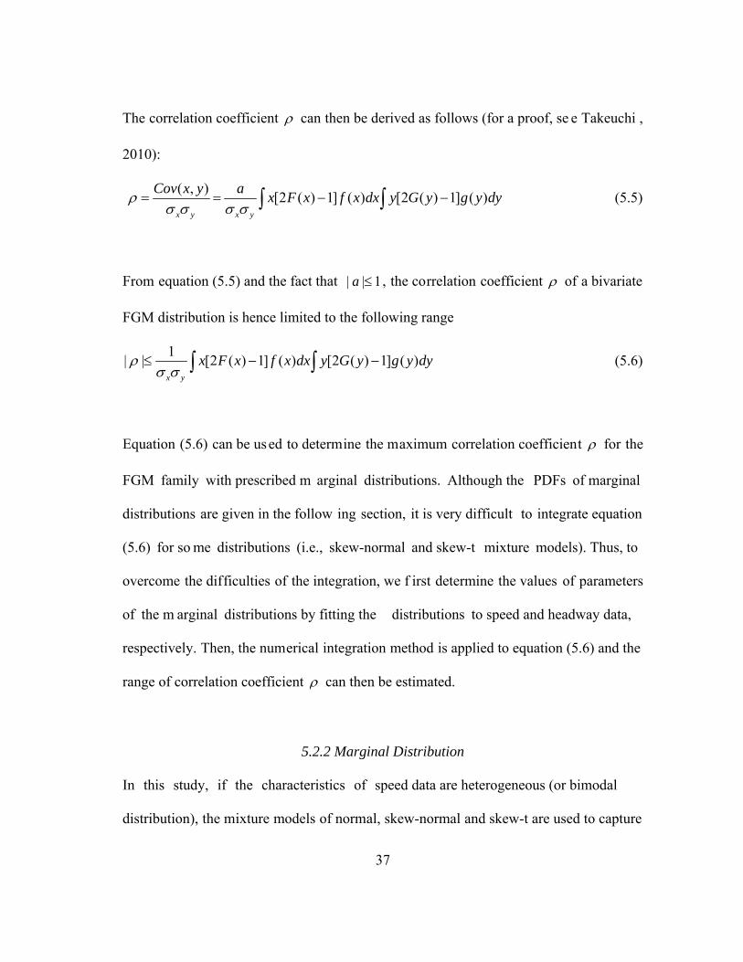
The correlation coefficient ρ can then be derived as follows (for a proof, se e Takeuchi ,

2010):

( , ) [2 ( ) 1] ( ) [2 ( ) 1] ( )x y x y

Cov x y a x F x f x dx y G y g y dyρσ σ σ σ

= = − −∫ ∫

(5.5)

From equation (5.5) and the fact that | | 1a ≤ , the correlation coefficient ρ of a bivariate

FGM distribution is hence limited to the following range

1| | [2 ( ) 1] ( ) [2 ( ) 1] ( )x y

x F x f x dx y G y g y dyρσ σ

≤ − −∫ ∫

(5.6)

Equation (5.6) can be used to determine the maximum correlation coefficient ρ for the

FGM family with prescribed m arginal distributions. Although the PDFs of marginal

distributions are given in the follow ing section, it is very difficult to integrate equation

(5.6) for so me distributions (i.e., skew-normal and skew-t mixture models). Thus, to

overcome the difficulties of the integration, we f irst determine the values of parameters

of the m arginal distributions by fitting the distributions to speed and headway data,

respectively. Then, the numerical integration method is applied to equation (5.6) and the

range of correlation coefficient ρ can then be estimated.

5.2.2 Marginal Distribution

In this study, if the characteristics of speed data are heterogeneous (or bimodal

distribution), the mixture models of normal, skew-normal and skew-t are used to capture

37

excess skewness, kurtosis and bim odality present in spe ed distribution. The m ixture

model is widely used in m odeling bimodal speed distribution to account for the

heterogeneity. To identify the va lues of parameters in the s elected distributions, the

Expectation/Conditional Maximization Either (ECME) algor ithm is chosen to estimate

the parameters of nor mal, skew-normal and ske w-t mixture models in this study. For

more details about the param eter estimation, interested readers could consult Zou and

Zhang (2011). All statistical analyses were carried out in Software R (2006).

For the headway m odel, three commonly used single distribution m odels are

investigated: gamma, lognormal and log-logi stic distributions. After determ ining the

statistical distribution governing headway, the next step is to estimate the parameters of

three proposed models. We also used the maximum likelihood estimation approach to

estimate the parameters. The three headway models are briefly introduced as follows.

The density function of a gamma distribution for headway can be written as:

1 ( / )

( | , )( )

xx ef xα β

αα βα β

− −

=Γ

(5.7)

( )E x αβ= (5.8)

2( )Var x αβ= (5.9)

where α is the shape param eter, β is the scale param eter, and ( )xΓ is the gamma

function.

38

The lognormal distribution has the following probability density function:

2

2(ln )

2 22

1( | , )2

x

f x ex

μσμ σ

πσ

−−

=

(5.10)

2

( ) exp( )2

E x σμ= +

(5.11)

2 2( ) (exp( ) 1) exp(2 )Var x σ μ σ= − + (5.12)

where μ and σ are the mean and stand ard deviation, respectively, of the variab le’s

natural logarithm.

The density function of a log-logistic distribution can be formulated as follows:

1

2

( / )( / )( | , )[1 ( / ) ]

xf xx

α

α

α β βα ββ

−

=+

(5.13)

/( )sin( / )

E x βπ απ α

=

for

1α >

(5.14)

2 2( ) (2( / ) / sin(2 / ) ( / ) / sin ( / ))Var x 2β π α π α π α π α= −

for

2α >

(5.15)

where α is the shape parameter, and β is the scale param eter and also th e median of

the distribution.

5.2.3 Goodness of Fit Statistics

To evaluate the goodness of fit of the select ed distributions for speed and headway data

as well as the bivariate distribution, the R2 and RMSE statistics are used in this study. R 2

statistic is a bin-specific test and measures the strength of linear relationship between the

expected and observed frequencies of the bins. The common definition of the R2 is 39

2 1 err

tot

SSRSS

= −

(5.16)

where represents the sum of squares of the residu als and measures the to tal

difference between the observed and expect ed frequency for all of the bins, and

denotes the total sum of squares and assess es the total difference between the observ ed

and average frequencies for all bins. R 2 statistic ranges from 0 to 1 and higher R 2 values

indicate a better fit.

errSS

totSS

The RMSE statistic is also bin-specific and has the following form:

err

T

SSRMSEN

=

(5.17)

where represents the sum of squares of residuals, and is the total number of

bins. Unlike the R 2 statistic, higher RMSE valu es indicate a poorer fit. R 2 can be

considered to be a m ore precise goodness of fit metric, because it uses the num ber of

non-empty bins in the equation, where the RMSE value makes use of the total number of

bins as a param eter in the equation. Note that when calculating the R 2 and RMSE

statistics for the bivariate distribution, reflects the total d ifference between th e

observed and expected frequency for all of the two-dimensional bins, and is the total

number of two-dimensional bins. For speed, the bin size of R 2 metric is fixed at 2 kph,

whereas for headway, the bin size is specified as 1 second. The RMSE m etric uses the

same bin size.

errSS TN

errSS

TN

40

5.3 Results and discussions

5.3.1 Marginal Models for Speed and Headway

Table 5.1 reports the estim ated parameters, R2 and RMS E values of different speed

models. Higher R2 and lower RMSE values ind icate a better overall fit. It can be seen

that all speed models have high R2 values. For the 24 hour sp eed data, the 4-component

normal mixture model is slightly better than the 2-component skew-t mixture model in

term of goodness of fit index. However, previous studies (Zou and Zhang, 2011) showed

that the 2-component skew-t mixture model can better account for heterogeneity in the

speed data. The histogram of speed data is gi ven in Figure 2 (a). Based on the graphical

visualization, all speed mode ls fit the 24-hour speed data well. In the m eantime, the

headway data were exam ined using gamm a, lognormal and log-logistic m odels. The

performance of headway m odels is not consistent. The estim ated parameters, R2 and

RMSE values are show n in Table 5.2. Based on the results, the log-logistic m odel has

the highest R 2 and low est RMSE values and the gamma m odel provides the least

satisfactory fitting performance. It is speculated that the gamma model may not be able

to capture the sharp peak present in the headway histogram. The histogram of headway

data is shown in Figure 2 (b). Note that speed and headway histograms have different

total number of bins ( ), respectively. And this e xplains that although the 4-

component normal mixture model for speed and the lognormal model for headway have

almost the same R2 values, the corresponding RMSE values differ significantly.

TN

41

Table 5.1 Parameter Estimation Results, R2 and RMSE Values for Speed Models Speed model Parameter group1 group2 group3 group4 R2 RMSE

4-component normal

mu 15.37 33.60 86.39 97.36

0.982 81.90 sigma 6.00 11.39 17.28 6.59

w 0.07 0.06 0.22 0.65

2-component skew-normal

mu 5.46 102.92

0.969 106.90 sigma 48.50 10.39

shape 20.15 -1.26

w 0.21 0.79

2-component skew-t

mu 6.95 101.71

0.979 87.65

sigma 22.22 8.89

shape 8.09 -1.07

nu 3.59 3.59

w 0.15 0.85

42

Figure 5.1 24-hour speed and headway histograms (a) speed (b) headway. 43

Table 5.2 Parameter Estimation Results, R2 and RMSE Values for Headway Models

Headway model Parameter R2 RMSE

gamma shape 1.34

0.853 528.53 scale 2.31

lognormal mu 0.71

0.981 191.71 sigma 0.93

log-logistic shape 2.05

0.999 40.47 scale 2.07

5.3.2 Correlation between Speed and Headway

As mentioned in the previous section, th e FGM approach has the limitation that the

correlation coefficients between the two variables should not exceed 1/3. For each

combination of marginal distributions of speed and headway, the m aximum correlation

coefficient is determ ined by num erically integrating equation (5.6) and the resu lts are

provided in Table 5.3. The Pearson correlation coefficient is calculated in this study to

verify the condition that it is sm aller than the maximum correlation c oefficients. The

Pearson correlation coefficien t is -0.0541. Since the Pears on correlation coefficient is

well below the maximum correlation coefficients provided in Table 5.3, the results show

that the weak correlation coefficient be tween speed and headway renders th e FGM

models suitable for our research on bivariate distributions.

44

Table 5.3 Maximum Correlation Coefficients for Each Marginal Distribution

gamma lognormal log-logistic

4-component normal 0.246 0.197 0.105

2-component skew-normal 0.248 0.199 0.106

2-component skew-t 0.240 0.193 0.103

45

One perspective to ass ess the co rrelation between speed and headway is to s tudy the

headway variation at different speed levels. In the study of Br ackstone et al. (2009), it is

revealed that there is a lim ited dependence of following headway on speed; the most

successful relationship fit of headway and sp eed is inverse relation ship. They also

suggested that drive r response can be split in to two regim es. The following tim e

headway is approxim ately constant when sp eed is above 15 m /s (54 kph) in the f irst

regime. In the second regim e when speed is below 15 m /s (54 kph), the following time

headway increases as the speed decreases. Following th e same procedure used in

Brackstone et al.’s st udy (2009), we divide the speed da ta (kph) into seven groups, and

the average headway for each speed group is given in Table 5.4. From Figure 1 (a), since

speed values in speed groups 1 through 4 ar e under 72 kph, it can be seen that speed

groups 1 through 4 consist of 4944 vehicles wi th recorded speed values observed under

congested traffic conditions. Thus , it is rea sonable to consider headway values

corresponding to those speed data in speed groups 1 through 4 as following headways. It

is observed that within these four speed groups, the mean of following headway

increases as the speed decrea ses, which is consistent with the f indings in the study by

Brackstone et al. (2009). On the othe r hand, for speed groups 5 through 7, 22975

vehicles are observed in off peak periods (uncongested traffic condition). Considering

few vehicles on the ro ad, vehicles can eas ily reach the free flow speed. As the s peed

grows higher, fewer vehicles are on the road and it is exp ected to see th at the headway

increases accordingly.

Table 5.4 Summary Statistics of Headway for Each Speed Group

Speed group

(kph)

Group

1

0-18

Group

2

18-36

Group

3

36-54

Group

4

54-72

Group

5

72-90

Group

6

90-108

Group

7

108+

Mean (s) 5.67 3.17 2.27 1.9 2.19 3.13 4.05

Min. (s) 1 0 0 0 0 0 0

Max. (s) 48 17 12 11 42 68 76

No. of vehicles 1501 1484 757 1202 4548 16698 1729

In order to further exa mine the co rrelation between speed and he adway on IH-35, we

study the determ inants of the individual vehicle speed and the individual vehicle

headway over a 24-hour period. It is im portant for us to note that the vehicle speed and

the vehicle headway will affect eac h other as well. Because of this interrela tionship,

formulating separate ordinary least square s regression m odels of speed and headway

would result in inef ficient parameter estimates. To addr ess this issue, Seemingly

Unrelated Regressions (SUR) es timation is u sed to a ccount for the direct correlation

46

between speed and headway. Adopting a sim ilar equation system used by Martchouk et

al. (2011), the speed and headway are determ ined in a simultaneous equation syste m

formalized as follows:

47

j S12

n

S jj

Speed C Headway Xβ β ε=

= + × + +∑

(5.18)

12

m

H i i Hi

Headway C Speed Yα α ε=

= + × + +∑

(5.19)

where Speed is the individual vehicle speed collected over a 24-hour period, Headway

represents the corresponding individual vehicle headway, jβ , for j=1,…,n, are estimated

parameters for speed equation, iα , for i=1,…,m, are estimated parameters for headway

equation, jX and are independent variables, and iY SC HC are constants, and Sε and

Hε are error terms. For the par ameter estimation, the SUR model is estimated using

systemfit package in the software R.

The SUR estimation results for speed and head way are provided in Tables 5.5 and 5.6,

respectively. In general, the speed and headw ay models fit the data w ell and the

coefficient estimates have plaus ible sign and are all statistical si gnificant at the 95%

level. The adjusted 2R for the vehicle speed m odel is 0.8387 and 0.2638 for the m odel

of vehicle headway.

In the model of individual vehicle speed (Table 5.5), the coefficient of variable headway

is -0.0727 which indicates that higher vehicl e headway slightly decreases vehicle speed.

This finding is consistent with the calculated Pearson correlation coefficient which is -

0.0541. For other variables, the increase of vari able vehicle length also results in slower

vehicle operating speed. The AM and PM p eak-hour variables can reduce the vehicle

speed. Since IH-35 experiences worst traffic congestion condition during afternoon peak

period, the vehicle speed drops significantly in the PM peak-hour. At night, drivers tend

to drive faster because fewer vehicles are on the road. In the model of individual vehicle

headway (Table 5.6), the coefficient of variable speed is -0.0058, which is also

consistent with the Pearson correlation coe fficient and shows that higher vehicle speed

slightly decreases vehicle headway. As e xpected, longer vehicle length and preceding

vehicle length result in larger veh icle headway, which is consistent with the finding by

Ye and Zhang (2009). The reason is th at trucks and buses generally accelerate and

decelerate more slowly than passenger cars. During the PM peak hours, vehicle headway

increases because most vehicles drove at 10-30 kph. Meanwhile, during the AM peak

hours, vehicle headway decreases because the flow almost reaches the capacity of th e

road and vehicles keep a m inimum following headway. For the variable night tim e, it

leads to higher vehicle headway. Note that based on the provided t-statistic values, the

effects of variables headway (in Table 5.5) and speed (in Table 5.6) are found to be

significant at the 95% level. The m odeling results from the SUR m odel suggest that

there is an inverse relationship between speed and headway. Overall, based on the

Pearson correlation coefficient, it can be seen that there is a weak dependence between

speed and headway, and this weak dependence renders the FGM models suitable for

constructing the joint distribution.

48

Table 5.5 Seemingly Unrelated Regression Model of Individual Vehicle Speed (in kph)

Variable Coefficient

Estimate

Standard

Error t-statistic

Constant 97.9186 0.1207 811.0385

Headway (second) -0.0727 0.0190 -3.8383

Vehicle length (ft) -0.1827 0.0139 -13.1477

AM peak-hour indicator (1 if time between

07:00-08:30, 0 otherwise) -22.5995 0.2103

-

107.4438

PM peak-hour indicator (1 if time between

15:30-19:30, 0 otherwise) -73.0294 0.1992

-

366.6260

Night-time indicator (1 if time between 00:00-

05:00, 0 otherwise)* 4.2229 0.3088 13.6765

Number of Observations 27919

Adjusted R-Squared 0.8387

* Due to the consistently heavy traffic on IH-35, the night time interval was selected

from 00:00 to 05:00.

49

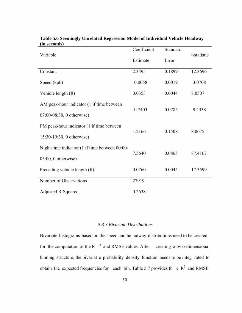
Table 5.6 Seemingly Unrelated Regression Model of Individual Vehicle Headway (in seconds)

Variable Coefficient

Estimate

Standard

Error t-statistic

Constant 2.3495 0.1899 12.3696

Speed (kph) -0.0058 0.0019 -3.0708

Vehicle length (ft) 0.0353 0.0044 8.0507

AM peak-hour indicator (1 if time between

07:00-08:30, 0 otherwise) -0.7403 0.0785 -9.4338

PM peak-hour indicator (1 if time between

15:30-19:30, 0 otherwise) 1.2166 0.1508 8.0675

Night-time indicator (1 if time between 00:00-

05:00, 0 otherwise) 7.5640 0.0865 87.4167

Preceding vehicle length (ft) 0.0760 0.0044 17.3599

Number of Observations 27919

Adjusted R-Squared 0.2638

5.3.3 Bivariate Distributions

Bivariate histograms based on the speed and he adway distributions need to be created

for the computation of the R 2 and RMSE values. After creating a tw o-dimensional

binning structure, the bivariat e probability density function needs to be integ rated to

obtain the expected frequencies for each bin. Table 5.7 provides th e R2 and RMSE

50

values based on the bivariate dist ributions. In Table 5.7, nine R 2 and RMSE values are

given for nine combinations of marginal distributions between speed and headway. The

combination of the 4-component norm al mixture distribution for speed and log-logistic

distribution for headway yields the highest R 2 and lowest RMSE values. The

combination of 2-com ponent skew-normal mixture distribution for speed and gamm a

distribution for headway gives the smallest R2 and largest RMSE values. For the purpose

of brevity, we only give the bivar iate histogram and the best f itted joint distribution in

Figure 3 (a) and (b). It can be observed that the trend of the bivariate histogram profile is

well captured by the FGM bivariate distribution.

Table 5.7 R2 and RMSE Values for Bivariate Distributions R2 gamma lognormal log-logistic



2-component skew-t 0.796 0.922 0.947

RMSE gamma lognormal log-logistic



2-component skew-t 16.901 10.425 8.59

51

Figure 5.2 Bivariate speed and headway histogram and fitted distribution: (a) bivariate speed and headway histogram; (b) fitted bivariate distribution.

52

5.3.4 Discussion

The modeling results are very interesting and deserve further discussion. Although the

bivariate distribution has been successfully c onstructed in this study, if we com pare the

R2 values in Tables 5.1 and 5.2 with those in Table 5.7, it can be found that the goodness

of fit index deteriorates slightly for bivari ate distributions as com pared with the one-

dimensional counterpart. The accu racy of marginal distributions is critical when using

the FGM approach to constr uct bivariate dist ributions, and satisfactory fitting

performance of bivariate distribution can be only achieved when appropriate m arginal

distributions are selected. Note that the R2 values for marginal distributions of speed and

headway are always higher than the R 2 values for corresponding bivariate distributions.

For example, the R2 value of gamma distribution for headway is 0.853, and any bivariate

distribution that includes the gamma distribution for headway has a R 2 value less than

0.8. Gamma distribution is the least perfor ming marginal distribution for headway, and

having gamma distribution as the m arginal distribution for headway lead to the least

performing bivariate distribution model. Therefore, it is necessary to provide the m ost

appropriate marginal distributions for sp eed and headway in order to construct a

satisfactory bivariate distribution using the FGM approach.

Traditionally, speed and headway are often not studied jointly in microscopic simulation

models. As a result, the sam e headway distribution may be assumed for different speed

levels and this assum ption neglects the pos sible variability of headway distribution

across speed values. To overcom e this potential problem associated with the traditional

53

approach, the constructed bivariate distribution in this study can be used to determine the

headway distribution for given speed values , and vice versa. For exam ple, given a

specific value of speed, the headway distribut ion corresponding to that speed value can

be derived based on equation (5.2). Thus, th e proposed method can be used to generate

vehicle speeds and v ehicle arrival times simultaneously by considering the dependence


There are several avenues for further work. First, since the applicability of the FGM

approach is affected by the correlation of the two variables, some other existing methods

to construct joint distributions such as m arginal transformation method, the mixing and

compounding methods and conditionally specified distributions (Balakrishnan and Lai,

2009) can be investigated. It would also be interesting to see the comparison of modeling

results by using different bi variate distribution constr uction approaches. Second,

realizing the effect of vehicle type o n the dependence between speed and headway, it is

useful to classify the traffic data base d on vehicle types and construct bivariate

distributions of speed and headway for each vehicle type separately (i.e., trucks and

passenger cars). Third, since the speed and headway data are site dependent and different

sites may have distinct traffic characteristics, more sites should be investigated to fully

explore the relationship between speed and headway.

54

5.4 Conclusions

In this stud y, the FG M approach is suc cessfully applied to cons truct the bivariate

distribution for speed and headway. The important findings and recommendations can be

summarized as follows. First, the modeling results based on empirical data indicate that

there is a weak inverse re lationship between the 24-hour speed and headway data, and

the weak dependence renders the FGM appro ach suitable for constructing bivariate

distributions. Second, the FGM is an eff ective approach to construct bivariate

distributions and when using the F GM, it is necessary to provide the most appropriate

marginal distributions for speed and head way in order to construct a satisfactory

bivariate distribution. Overa ll, as m entioned in the disc ussion section, the proposed

FGM approach can consider the dependence between speed and headway which is often

neglected in traditional m icroscopic simulation models. Thus, this study provides a

framework for developing microscopic simulation models to generate vehicle speeds and

vehicle arrival times simultaneously. In addition, the statistical methods used to establish

the relationship between speed an d headway can be further applied to speed and

headway data from multiple areas and locations.

55

CHAPTER VI

SUMMARY AND CONCLUSIONS

6.1 Summary

Traditionally, traffic variab les (speed and headway) are often not studied jointly in

microscopic simulation models. One im portant flaw asso ciated with the traditional

approach is that the sim ulated samples based on the independence assum ption usually

fail to consider the em pirical dependence between traffic variab les. To overcome this

potential problem associated with the trad itional approach, it is n ecessary to cons truct

bivariate distributions to model vehicle speed and headway simultaneously.

The research first examined the dependence structure between speed and headway using

three measures of dependence (i.e., Pearson correlation coefficient, Spearman’s rho and

Kendall’s tau). The research proposed th e skew-t mixture m odels to cap ture

heterogeneity present in speed distribution. To develop a bivari ate distribution for

capturing the dependence, the FGM m ethod was applied to the 24-hour speed and

headway data.

6.2 Conclusions

Based on the modeling results from this rese arch, we drew some important conclusions,

which are listed as follows:

56

1. The proposed skew-t m ixture models can reasonable account for heterogeneity

problem in freeway vehicle speed data. Fini te mixture of skew-t distributions can

significantly improve the goodness of fit of speed data. The m ethodology developed in

this research can be used in analyzing the characteristics of freeway speed data.

Considering that many traffic analytical and simulation models use speed as an input for

travel time and level of service determ ination, the developed models can generate more

accurate speed value as the input and help improving the reliability of the analysis output.

2. There exists weak dependence between speed and headw ay. The dep endence

between speed and headway is strongest under the most congested traffic condition. The

bivariate model can provide a satisfactory fit to th e multimodal speed and headway

distribution. The proposed m ethodology can overcome the correlation problem

associated with the traditional approach.

6.3 Future Research

This research proposes the FGM approach to construct bivariate distributions to describe

the characteristics of speed and headway, and there are some avenues for future work.

1. A better understanding of speed and headway distributions and its dependence

structure can help operational analysis of a f reeway facility. In future, since the s peed

and headway data are site dependent and di fferent sites m ay have distinct traffic

characteristics, multiple locations should be investigated to fully explore the relationship


57

2. Traffic headway includes time headway and distance headway, which are closely

related to each other and bot h vary depending on speed an d traffic condition. Distance

headway is also an im portant microscopic traffic variable and one in fluential factor in

the car following model. Some studies have shown that there exists positive dependence

between distance headway and speed. Thus, if the distance h eadway data is available in

this study, we can further investigate the dependence struct ure between distance

headway and speed. The findings from further analysis may contribute to the existing car

following theory.

3. In some popular traffic sim ulation models (i.e., CORSIM, Sim Traffic and

VISSIM), vehicles are usually generated on the basis of a ce rtain headway distribution.

CORSIM considers three types of vehicle entry headway generation distributions:

uniform, normal and Erlang distributions. The negative exponential di stribution is used

in VISSIM and SimTraffic. The current simulation protocols in these microscopic traffic

simulation models fail to consider the dependence between speed and headway. Thus, in

the future, the bivariate distributions can be used in these traffic simulation models to

generate more accurate speed and headway of entry vehicle.

58

REFERENCES

AZZALINI, A. 1985. A Class of Distributions Which Includes the Normal Ones.

Scandinavian Journal of Statistics, 12, 171-178. AZZALINI, A. & CAPITANIO, A. 2003. Distributions generated by perturbation of

symmetry with emphasis on a multivariate skew t-distribution. Journal of the Royal Statistical Society Series B-Statistical Methodology, 65, 367-389.

BASSO, R. M., LACHOS, V. H., CABRAL, C. R. B. & GHOSH, P. 2010. Robust mixture modeling based on scale mixtures of skew-normal distributions. Computational Statistics & Data Analysis, 54, 2926-2941.

BHAT, C. R. & ELURU, N. 2009. A copula-based approach to accommodate residential self-selection effects in travel behavior modeling. Transportation Research Part B-Methodological, 43, 749-765.

BIERNACKI, C., CELEUX, G. & GOVAERT, G. 2000. Assessing a mixture model for clustering with the integrated completed likelihood. Pattern Analysis and Machine Intelligence, IEEE Transactions on, 22, 719-725.

BRACKSTONE, M., WATERSON, B. & MCDONALD, M. 2009. Determinants of following headway in congested traffic. Transportation Research Part F-Traffic Psychology and Behaviour, 12, 131-142.

COWAN, R. J. 1975. Useful Headway Models. Transportation Research, 9, 371-375. DEMPSTER, A. P., LAIRD, N. M. & RUBIN, D. B. 1977. Maximum Likelihood from

Incomplete Data Via Em Algorithm. Journal of the Royal Statistical Society Series B-Methodological, 39, 1-38.

DEY, P. P. & CHANDRA, S. 2009. Desired Time Gap and Time Headway in Steady-State Car-Following on Two-Lane Roads. Journal of Transportation Engineering-Asce, 135, 687-693.

DEY, P. P., CHANDRA, S. & GANGOPADHAYA, S. 2006. Speed distribution curves under mixed traffic conditions. Journal of Transportation Engineering-Asce, 132, 475-481.

ERDEM, E. & SHI, J. 2011. Comparison of bivariate distribution construction approaches for analysing wind speed and direction data. Wind Energy, 14, 27-41.

FR HWIRTH-SCHNATTER, S. 2006. Finite mixture and Markov switching models. GERLOUGH, D. L. & HUBER, M. J. 1976. Traffic flow theory. HAIGHT, F. A. 1965. Mathematical theories of traffic flow. HAIGHT, F. A. & MOSHER, W. W. 1962. A practical method for improving the

accuracy of vehicular speed distribution measurements. Highway Research Board Bulletin.

HOOGENDOORN, S. P. & BOVY, P. H. 1998. New estimation technique for vehicle-type-specific headway distributions. Transportation Research Record: Journal of the Transportation Research Board, 1646, 18-28.

HUANG, J. & KOTZ, S. 1999. Modifications of the Farlie-Gumbel-Morgenstern distributions. A tough hill to climb. Metrika, 49, 135-145.

59

JOHNSON, N. L. & KOTZ, S. 1977. On some generalized farlie-gumbel-morgenstern distributions-II regression, correlation and further generalizations. Communications in Statistics-Theory and Methods, 6, 485-496.

JUN, J. 2010. Understanding the variability of speed distributions under mixed traffic conditions caused by holiday traffic. Transportation Research Part C-Emerging Technologies, 18, 599-610.

KO, J. & GUENSLER, R. L. Characterization of congestion based on speed distribution: a statistical approach using Gaussian mixture model. Transportation Research Board Annual Meeting, 2005. Citeseer.

LEONG, H. The distribution and trend of free speeds on two lane two way rural highways in New South Wales. Australian Road Research Board (ARRB) Conference, 4th, 1968, Melbourne, 1968.

LIN, T. I., LEE, J. C. & HSIEH, W. J. 2007. Robust mixture modeling using the skew t distribution. Statistics and Computing, 17, 81-92.

LUTTINEN, R. 1992. Statistical properties of vehicle time headways. Transportation research record.

LUTTINEN, R. T. 1999. Properties of Cowan's M3 headway distribution. Transportation Research Record: Journal of the Transportation Research Board, 1678, 189-196.

MARTCHOUK, M., MANNERING, F. & BULLOCK, D. 2010. Analysis of freeway travel time variability using Bluetooth detection. Journal of Transportation Engineering, 137, 697-704.

MCLEAN, J. Observed speed distributions and rural road traffic operations. Australian Road Research Board Conference Proc, 1979.

PARK, B. J., ZHANG, Y. L. & LORD, D. 2010. Bayesian mixture modeling approach to account for heterogeneity in speed data. Transportation Research Part B-Methodological, 44, 662-673.

SCHUCANY, W. R., PARR, W. C. & BOYER, J. E. 1978. Correlation Structure in Farlie-Gumbel-Morgenstern Distributions. Biometrika, 65, 650-653.

TAIEB-MAIMON, M. & SHINAR, D. 2001. Minimum and comfortable driving headways: Reality versus perception. Human Factors: The Journal of the Human Factors and Ergonomics Society, 43, 159-172.

TAKEUCHI, T. T. 2010. Constructing a bivariate distribution function with given marginals and correlation: application to the galaxy luminosity function. Monthly Notices of the Royal Astronomical Society, 406, 1830-1840.

WASIELEWSKI, P. 1979. Car-following headways on freeways interpreted by the semi-Poisson headway distribution model. Transportation Science, 13, 36-55.

WINSUM, W. V. & HEINO, A. 1996. Choice of time-headway in car-following and the role of time-to-collision information in braking. Ergonomics, 39, 579-592.

YE, F. & ZHANG, Y. 2009. Vehicle type-specific headway analysis using freeway traffic data. Transportation Research Record: Journal of the Transportation Research Board, 2124, 222-230.

60

61

YE, Z., ZHANG, Y. & MIDDLETON, D. R. 2006. Unscented Kalman filter method for speed estimation using single loop detector data. Transportation Research Record: Journal of the Transportation Research Board, 1968, 117-125.

YIN, S. C., LI, Z. H., ZHANG, Y., YAO, D., SU, Y. L. & LI, L. 2009. Headway Distribution Modeling with Regard to Traffic Status. 2009 Ieee Intelligent Vehicles Symposium, Vols 1 and 2, 1057-1062.

ZHANG, G., WANG, Y., WEI, H. & CHEN, Y. 2007. Examining headway distribution models with urban freeway loop event data. Transportation Research Record: Journal of the Transportation Research Board, 1999, 141-149.

ZHANG, Y., XIE, Y. & YE, Z. Estimation of large truck volume using single loop detector data. Transportation Research Board 87th Annual Meeting, 2008.

ZOU, Y. & ZHANG, Y. 2011. Use of skew-normal and skew-t distributions for mixture modeling of freeway speed data. Transportation Research Record: Journal of the Transportation Research Board, 2260, 67-75.

Documents

1. Report No. 2. Government Accession No. SWUTC/13 ... knowledge of speed and headway distributions is essential in microscopic traffic flow studies because speed and headway are both