1

Rational Consumer Choice

APEC 3001

Summer 2007Readings: Chapter 3 & Appendix in Frank

2

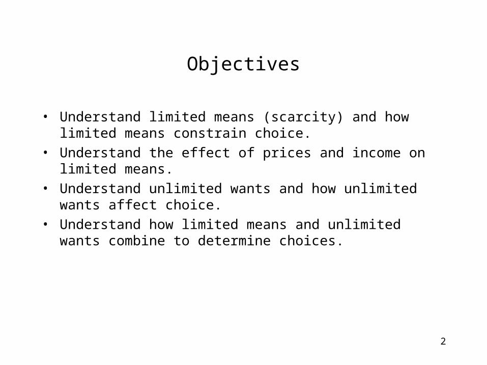
Objectives

• Understand limited means (scarcity) and how limited means constrain choice.

• Understand the effect of prices and income on limited means.

• Understand unlimited wants and how unlimited wants affect choice.

• Understand how limited means and unlimited wants combine to determine choices.

3

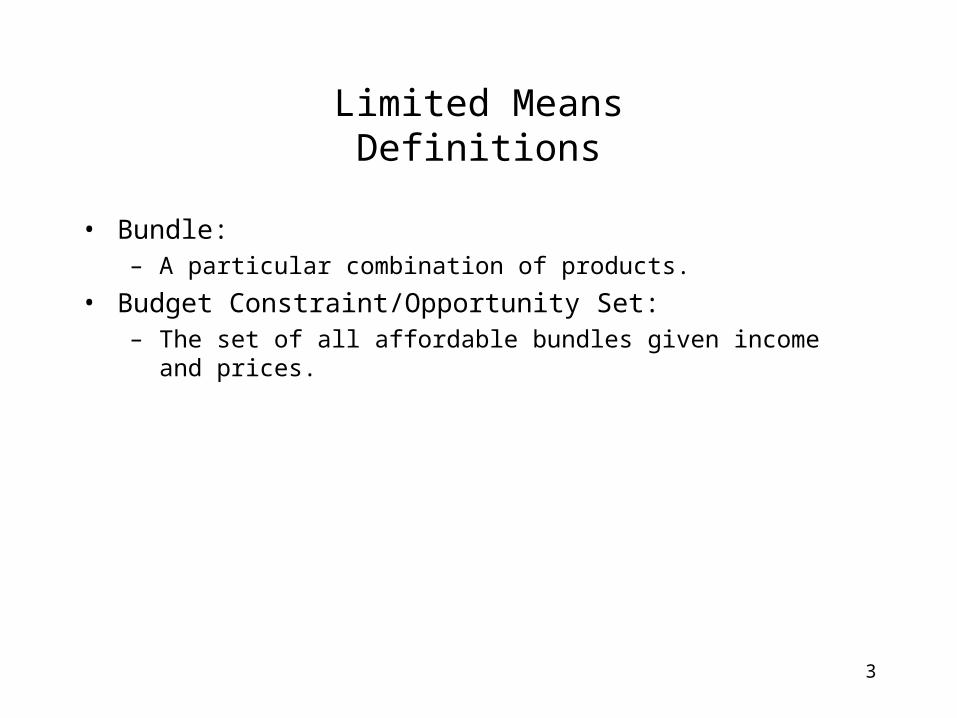
Limited MeansDefinitions

• Bundle:– A particular combination of products.

• Budget Constraint/Opportunity Set: – The set of all affordable bundles given income and prices.

4

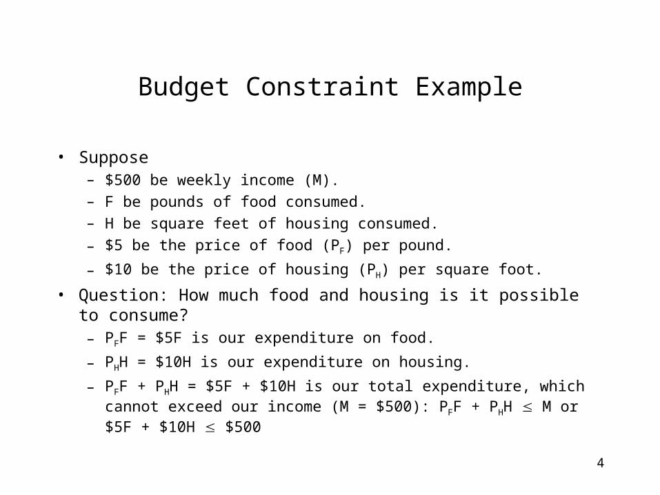
Budget Constraint Example

• Suppose– $500 be weekly income (M).

– F be pounds of food consumed.

– H be square feet of housing consumed.

– $5 be the price of food (PF) per pound.

– $10 be the price of housing (PH) per square foot.

• Question: How much food and housing is it possible to consume?– PFF = $5F is our expenditure on food.

– PHH = $10H is our expenditure on housing.

– PFF + PHH = $5F + $10H is our total expenditure, which cannot exceed our income (M = $500): PFF + PHH M or $5F + $10H $500

5

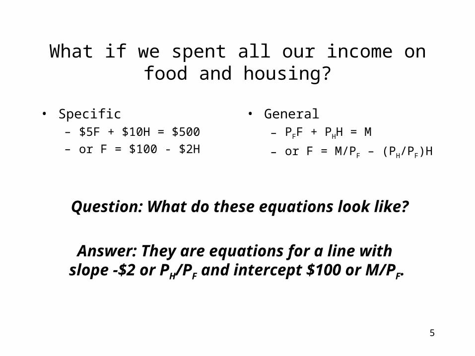
What if we spent all our income on food and housing?

• Specific– $5F + $10H = $500

– or F = $100 - $2H

• General– PFF + PHH = M

– or F = M/PF – (PH/PF)H

Question: What do these equations look like?

Answer: They are equations for a line with slope -$2 or PH/PF and intercept $100 or M/PF.

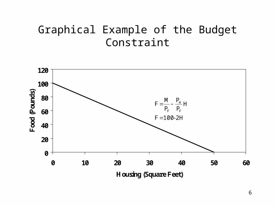
6

0

20

40

60

80

100

120

0 10 20 30 40 50 60

Housing (Square Feet)

Foo

d (P

ound

s)Graphical Example of the Budget Constraint

2H-100F

HP

P

P

MF

F

H

F

7

Questions

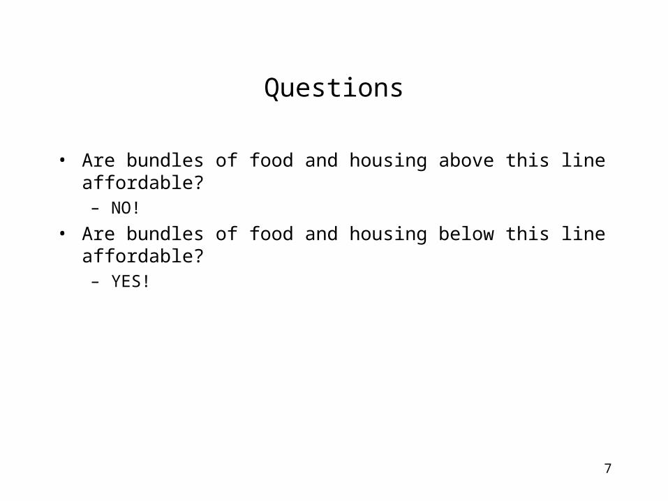
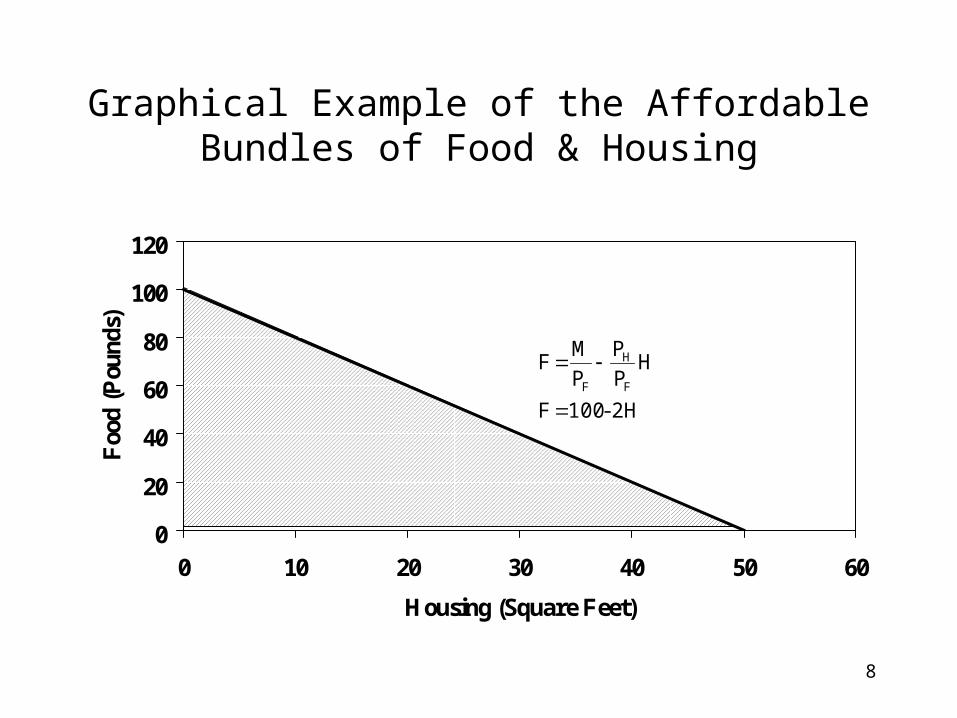
• Are bundles of food and housing above this line affordable?– NO!

• Are bundles of food and housing below this line affordable?– YES!

8

0

20

40

60

80

100

120

0 10 20 30 40 50 60

Housing (Square Feet)

Foo

d (P

ound

s)Graphical Example of the Affordable Bundles of

Food & Housing

2H-100F

HP

P

P

MF

F

H

F

9

Useful things to know about the budget constraint.

• The slope of the budget constraint tells us how much food we need to give up if we want to consume more housing, while still spending all of our income.

• The y intercept tell us how much food we can consume if we only consume food.

• The x intercept tells us how much housing we can consume if we only consume housing.

10

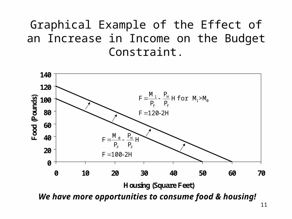
Effect of Income on Limited Means

• Question: What happens to the budget constraint if we increase weekly income from $500 to $600?

• Answer: – Specific: $5F + $10H = $600, so F = 120 – 2H.

– General: PFF + PHH = M1 instead of M0 where M1 > M0, so F = M1/PF – (PH/PF)H.

11

0

20

40

60

80

100

120

140

0 10 20 30 40 50 60 70

Housing (Square Feet)

Foo

d (P

ound

s)Graphical Example of the Effect of an Increase in

Income on the Budget Constraint.

2H-100F

HP

P

P

MF

F

H

F

0

2H-120F

HP

P

P

MF

F

H

F

1

for M1>M0

We have more opportunities to consume food & housing!

12

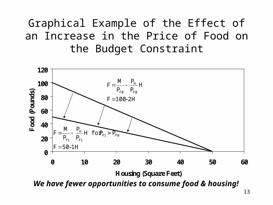
Effect of Prices on Limited Means

• Question: What happens to the budget constraint if we increase the price of food from $5 to $10?

• Answer: – Specific: $10F + $10H = $500, so F = 50 – 1H.

– General: PF1F + PHH = M1 instead of PF0 where PF1 > PF0, so F = M1/PF1 – (PH/PF1)H.

13

0

20

40

60

80

100

120

0 10 20 30 40 50 60

Housing (Square Feet)

Foo

d (P

ound

s)Graphical Example of the Effect of an Increase in the

Price of Food on the Budget Constraint

2H-100F

HP

P

P

MF

0F

H

0F

1H-50F

PPfor HP

P

P

MF 0F1F

1F

H

1F

We have fewer opportunities to consume food & housing!

14

Budget Constraints Can Be More Complicated

• Examples– Budget Constraints With a Food Stamp Program

– Budget Constraints With Two Tiered Pricing

15

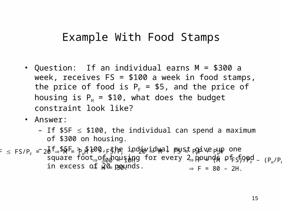
Example With Food Stamps

• Question: If an individual earns M = $300 a week, receives FS = $100 a week in food stamps, the price of food is PF = $5, and the price of housing is PH = $10, what does the budget constraint look like?

• Answer:– If $5F $100, the individual can spend a maximum of $300 on housing.

– If $5F > $100, the individual must give up one square foot of housing for every 2 pounds of food in excess of 20 pounds.

F FS/PF = 20 M = PHH 300 = 10H H = 30.

F > FS/PF = 20 M + FS = PFF + PHH F = (M + FS)/PF – (PH/PF)H F = 80 – 2H.

16

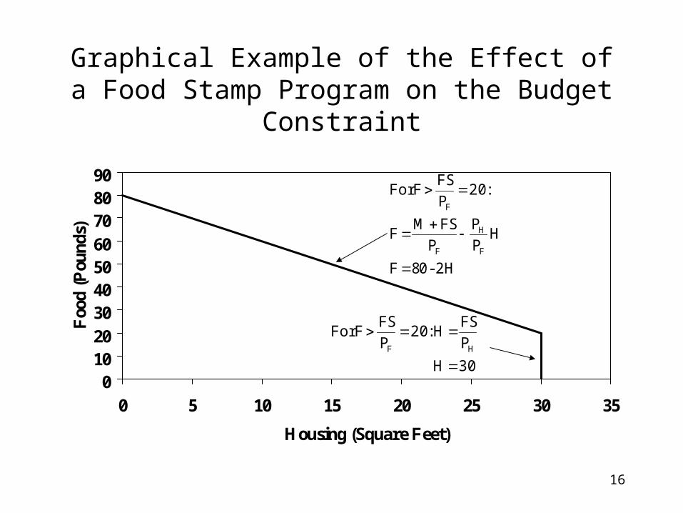
0102030405060708090

0 5 10 15 20 25 30 35

Housing (Square Feet)

Foo

d (P

ound

s)Graphical Example of the Effect of a Food Stamp

Program on the Budget Constraint

2H-08F

HP

P

P

FSMF

:20P

FSFFor

F

H

F

F

30H

P

FSH :20

P

FSFFor

HF

17

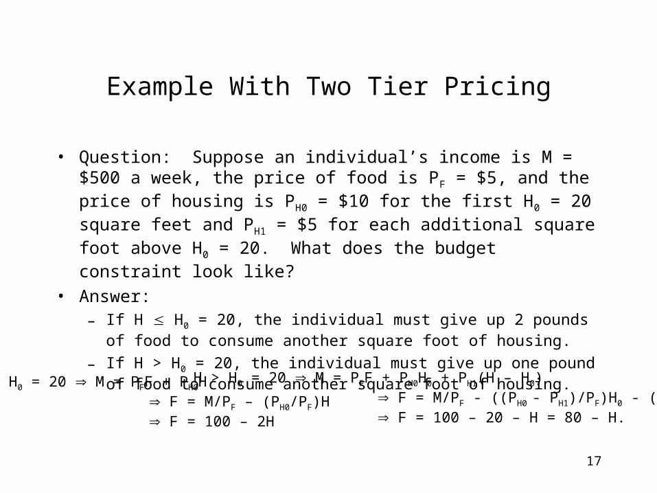
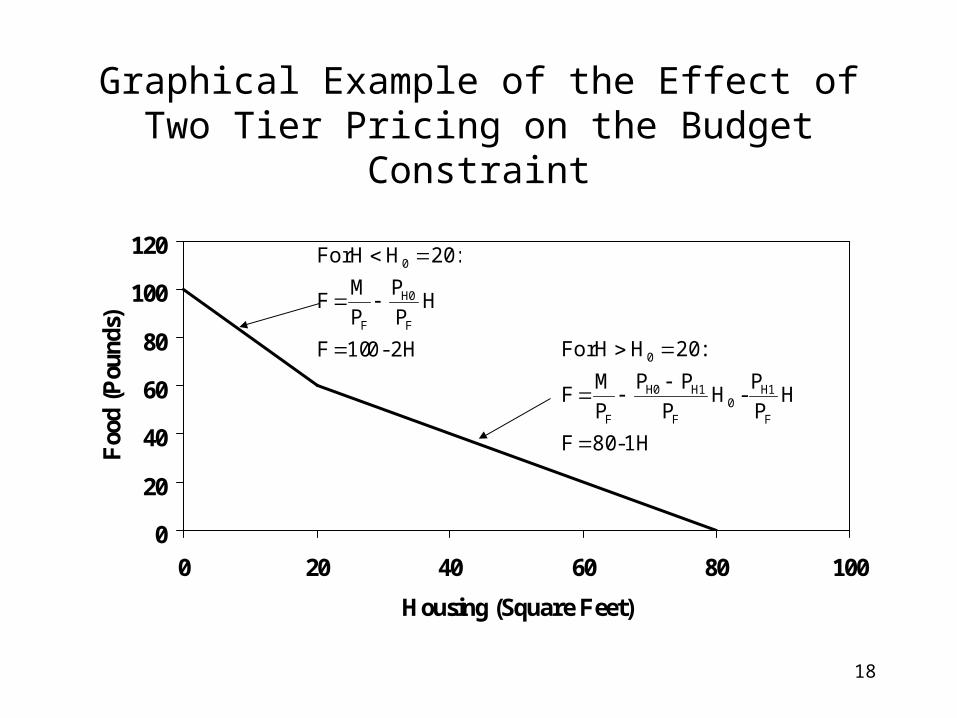
Example With Two Tier Pricing

• Question: Suppose an individual’s income is M = $500 a week, the price of food is PF = $5, and the price of housing is PH0 = $10 for the first H0 = 20 square feet and PH1 = $5 for each additional square foot above H0 = 20. What does the budget constraint look like?

• Answer:– If H H0 = 20, the individual must give up 2 pounds of food to consume

another square foot of housing.

– If H > H0 = 20, the individual must give up one pound of food to consume another square foot of housing.

H < H0 = 20 M = PFF + PH0H F = M/PF – (PH0/PF)H F = 100 – 2H

H > H0 = 20 M = PFF + PH0H0 + PH1(H – H0) F = M/PF - ((PH0 - PH1)/PF)H0 - (PH1/PF)H F = 100 – 20 – H = 80 – H.

18

0

20

40

60

80

100

120

0 20 40 60 80 100

Housing (Square Feet)

Foo

d (P

ound

s)Graphical Example of the Effect of Two Tier Pricing

on the Budget Constraint

2H-010F

HP

P

P

MF

:20HHFor

F

H0

F

0

1H-80F

HP

P-H

P

PP

P

MF

:20HHFor

F

H10

F

H1H0

F

0

19

Unlimited Wants

• Definition– Preference Ordering: A scheme whereby the consumer ranks all possible

consumption bundles in order of preference.

• Fundamental Assumptions of Preference Orderings– Completeness

– More Is Better (Nonsatiation)

– Transitivity

– Convexity

20

Completeness

• For every possible pair of consumption bundles (i) and (ii):– (i) is more satisfying than (ii),

– (i) is less satisfying than (ii),

– or (i) is just as satisfying as (ii).

The completeness property is violated when an individual cannot compare (i) and (ii).

21

More Is Better (Nonsatiation)

• If (i) has more of some products and at least the same amount of all other products as (ii),– then (i) is more satisfying than (ii).

22

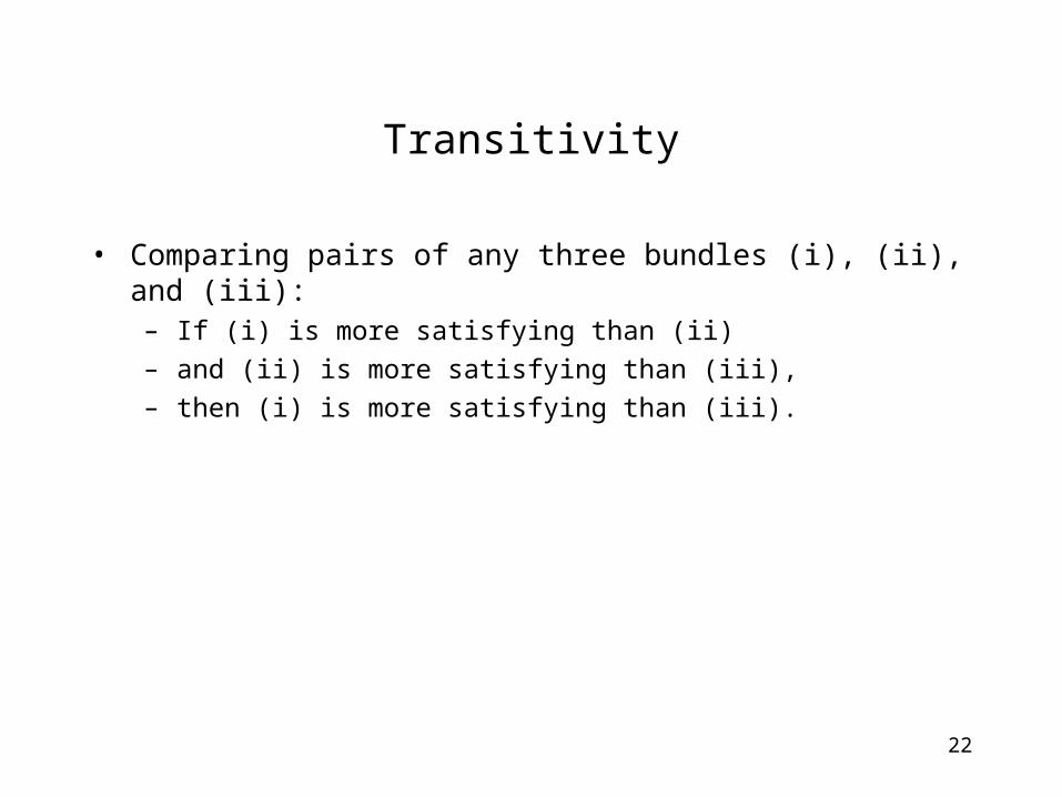
Transitivity

• Comparing pairs of any three bundles (i), (ii), and (iii):– If (i) is more satisfying than (ii)

– and (ii) is more satisfying than (iii),

– then (i) is more satisfying than (iii).

23

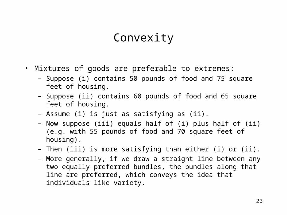
Convexity

• Mixtures of goods are preferable to extremes:– Suppose (i) contains 50 pounds of food and 75 square feet of housing.

– Suppose (ii) contains 60 pounds of food and 65 square feet of housing.

– Assume (i) is just as satisfying as (ii).

– Now suppose (iii) equals half of (i) plus half of (ii) (e.g. with 55 pounds of food and 70 square feet of housing).

– Then (iii) is more satisfying than either (i) or (ii).

– More generally, if we draw a straight line between any two equally preferred bundles, the bundles along that line are preferred, which conveys the idea that individuals like variety.

24

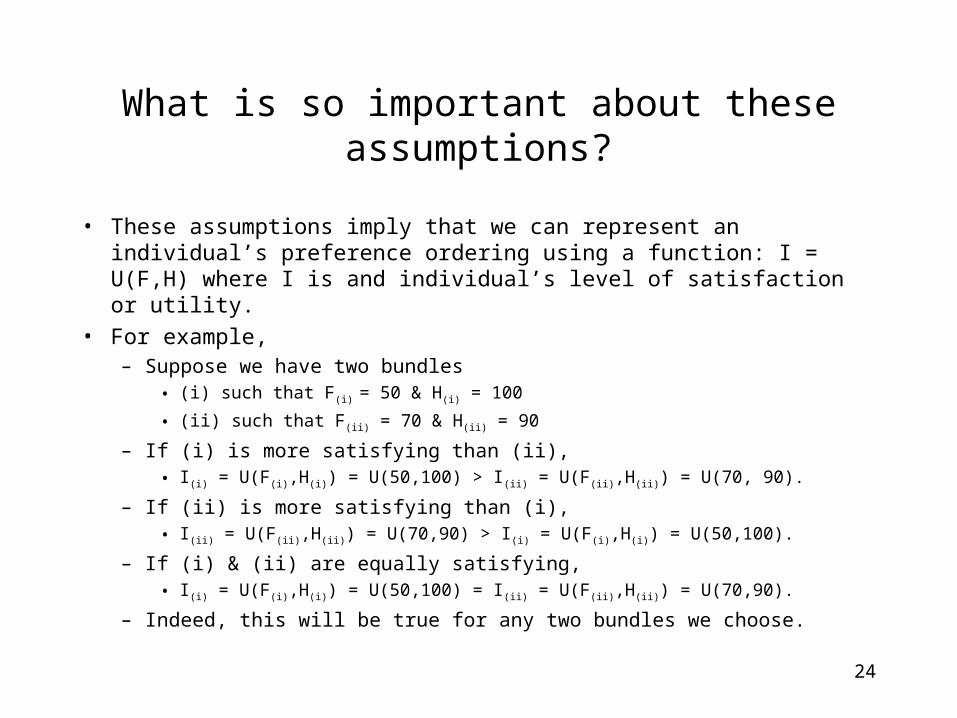
What is so important about these assumptions?

• These assumptions imply that we can represent an individual’s preference ordering using a function: I = U(F,H) where I is and individual’s level of satisfaction or utility.

• For example,– Suppose we have two bundles

• (i) such that F(i) = 50 & H(i) = 100

• (ii) such that F(ii) = 70 & H(ii) = 90

– If (i) is more satisfying than (ii), • I(i) = U(F(i),H(i)) = U(50,100) > I(ii) = U(F(ii),H(ii)) = U(70, 90).

– If (ii) is more satisfying than (i), • I(ii) = U(F(ii),H(ii)) = U(70,90) > I(i) = U(F(i),H(i)) = U(50,100).

– If (i) & (ii) are equally satisfying, • I(i) = U(F(i),H(i)) = U(50,100) = I(ii) = U(F(ii),H(ii)) = U(70,90).

– Indeed, this will be true for any two bundles we choose.

25

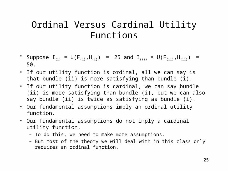
Ordinal Versus Cardinal Utility Functions

• Suppose I(i) = U(F(i),H(i)) = 25 and I(ii) = U(F(ii),H(ii)) = 50.

• If our utility function is ordinal, all we can say is that bundle (ii) is more satisfying than bundle (i).

• If our utility function is cardinal, we can say bundle (ii) is more satisfying than bundle (i), but we can also say bundle (ii) is twice as satisfying as bundle (i).

• Our fundamental assumptions imply an ordinal utility function.

• Our fundamental assumptions do not imply a cardinal utility function. – To do this, we need to make more assumptions.

– But most of the theory we will deal with in this class only requires an ordinal function.

26

Important Implication of Ordinal Utility

• We cannot make interpersonal comparisons!– If Mason’s utility from consuming 50 pounds of food & 100 square feet of

housing is 75 and Spencer’s utility from consuming the same bundle of products is 50, we cannot say this bundle makes Mason more satisfied than Spencer.

27

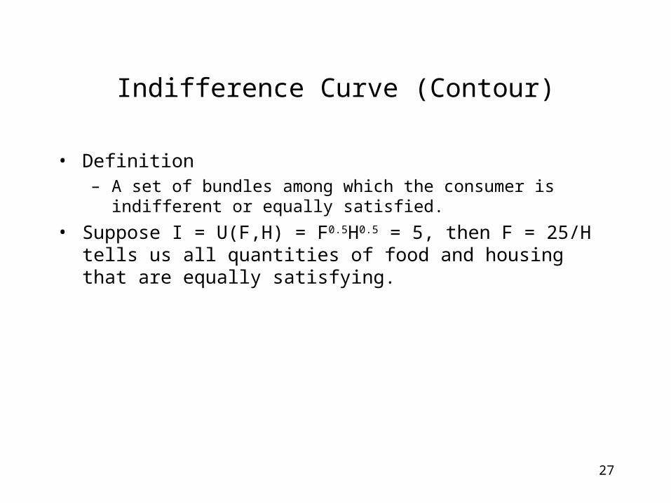
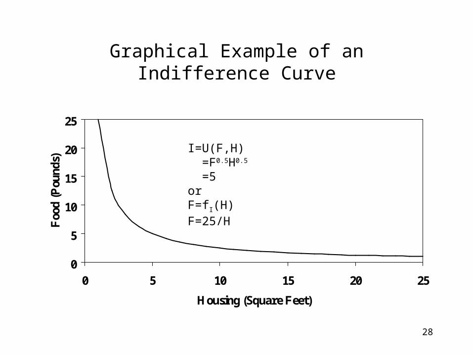
Indifference Curve (Contour)

• Definition– A set of bundles among which the consumer is indifferent or equally

satisfied.

• Suppose I = U(F,H) = F0.5H0.5 = 5, then F = 25/H tells us all quantities of food and housing that are equally satisfying.

28

Graphical Example of an Indifference Curve

0

5

10

15

20

25

0 5 10 15 20 25

Housing (Square Feet)

Foo

d (P

ound

s)

I=U(F,H) =F0.5H0.5

=5orF=fI(H)F=25/H

29

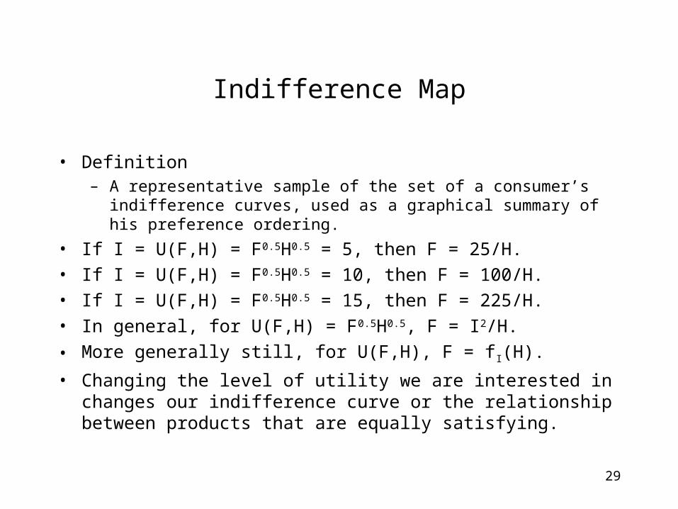
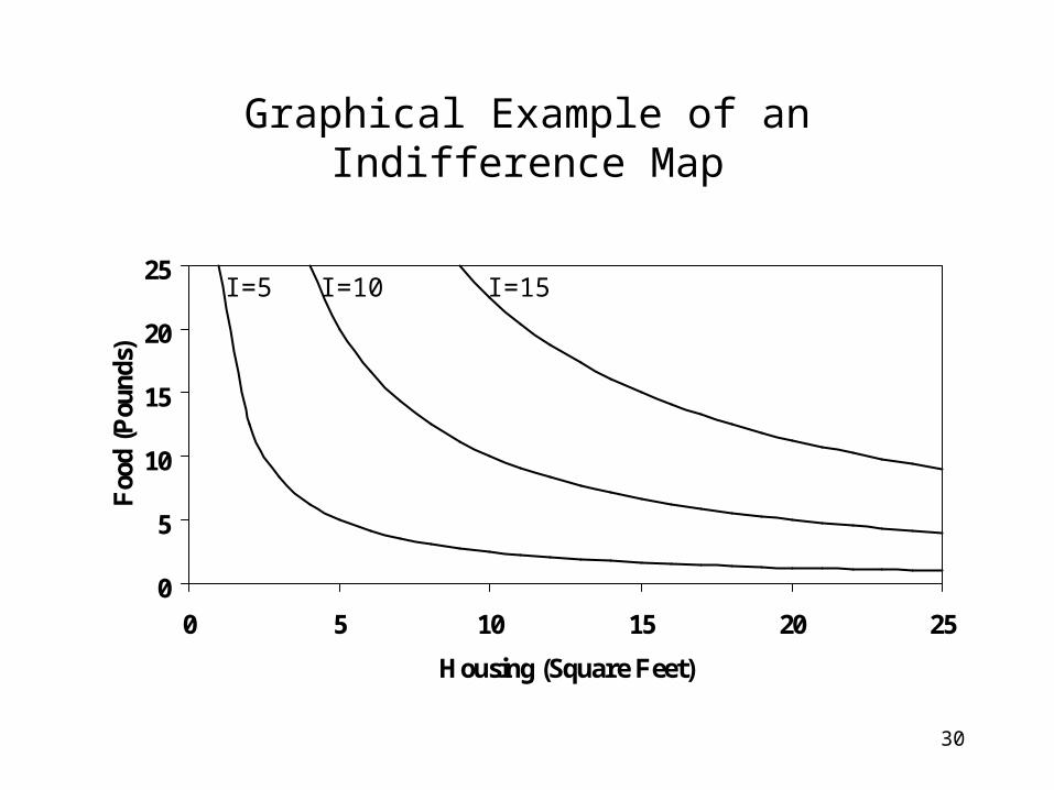
Indifference Map

• Definition– A representative sample of the set of a consumer’s indifference curves,

used as a graphical summary of his preference ordering.

• If I = U(F,H) = F0.5H0.5 = 5, then F = 25/H.

• If I = U(F,H) = F0.5H0.5 = 10, then F = 100/H.

• If I = U(F,H) = F0.5H0.5 = 15, then F = 225/H.

• In general, for U(F,H) = F0.5H0.5, F = I2/H.

• More generally still, for U(F,H), F = fI(H).

• Changing the level of utility we are interested in changes our indifference curve or the relationship between products that are equally satisfying.

30

Graphical Example of an Indifference Map

0

5

10

15

20

25

0 5 10 15 20 25

Housing (Square Feet)

Foo

d (P

ound

s)

I=5 I=10 I=15

31

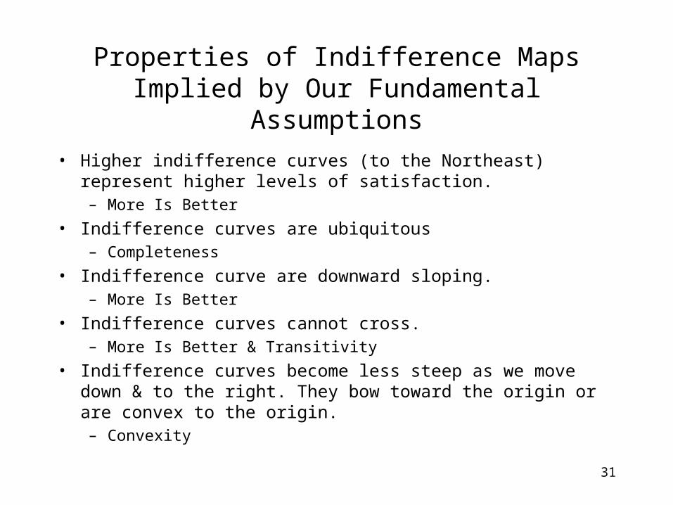
Properties of Indifference Maps Implied by Our Fundamental Assumptions

• Higher indifference curves (to the Northeast) represent higher levels of satisfaction.– More Is Better

• Indifference curves are ubiquitous – Completeness

• Indifference curve are downward sloping.– More Is Better

• Indifference curves cannot cross.– More Is Better & Transitivity

• Indifference curves become less steep as we move down & to the right. They bow toward the origin or are convex to the origin.– Convexity

32

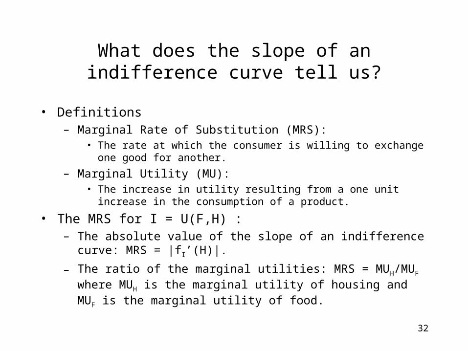
What does the slope of an indifference curve tell us?

• Definitions– Marginal Rate of Substitution (MRS):

• The rate at which the consumer is willing to exchange one good for another.

– Marginal Utility (MU): • The increase in utility resulting from a one unit increase in the consumption of

a product.

• The MRS for I = U(F,H) : – The absolute value of the slope of an indifference curve: MRS = |fI’(H)|.

– The ratio of the marginal utilities: MRS = MUH/MUF where MUH is the marginal utility of housing and MUF is the marginal utility of food.

33

Graphical Example of the Marginal Rate of Substitution

0

5

10

15

20

25

0 5 10 15 20 25

Housing (Square Feet)

Foo

d (P

ound

s)

I=10

F = 12.5 and H = 8

F

SMRS=|slope| = - F/ = MUH/MUF

34

Calculus Become Really Useful Here

• Suppose I = U(F,H) = F0.5H0.5.– For I = 10, F = f10(H) = 100/H, such that MRS = |f10’(H)| = |-100/H2| =

100/H2.• So, if H = 4, MRS = 100/16 = 6.25.

– Generally, MUH = UH(F,H) = 0.5F0.5H-0.5 = 0.5(F/H)0.5 and MUF = UF(F,H) = 0.5F-0.5H0.5 = 0.5(H/F)0.5, such that MRS = MUH/MUF = (0.5(F/H)0.5)/(0.5(H/F)0.5) = F/H.

• So, if I = 10 and H = 4, F = 100/4 = 25 such that MRS = 25/4 =6.25.

Recall from our Math Review:

H

HF,UHF,Uand

F

HF,UHF,U HF

35

Combining Limited Means & Unlimited Wants

• The budget constraint tells us the bundles we can afford.

• Indifference maps tell us which bundles we prefer to consume.

• If we bring the two together we can find the most satisfying bundle that is still affordable. We will call this bundle the best feasible bundle.

36

0

20

40

60

80

100

120

0 10 20 30 40 50 60

Housing (Square Feet)

Foo

d (P

ound

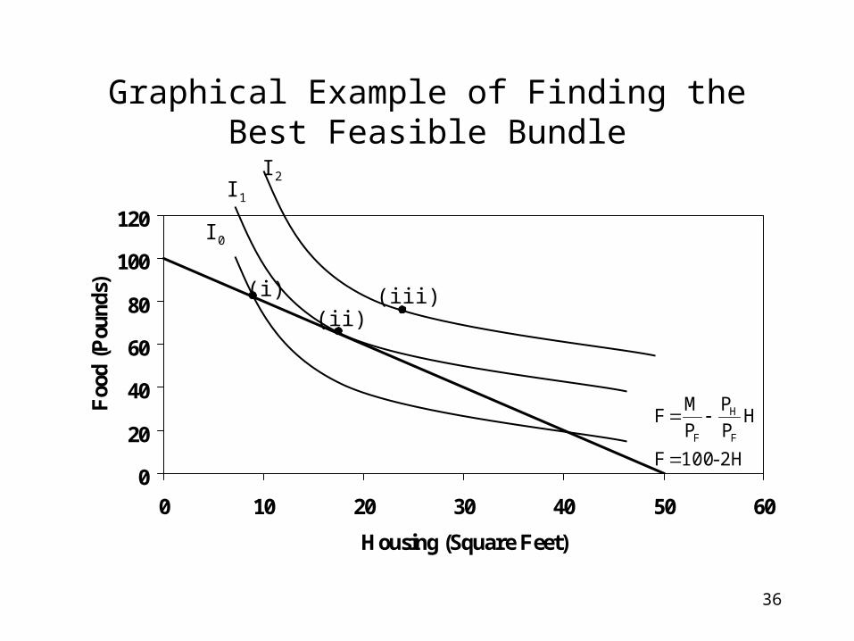
s)Graphical Example of Finding the Best Feasible

Bundle

2H-100F

HP

P

P

MF

F

H

F

I2I1

I0

(i)

(ii)(iii)

37

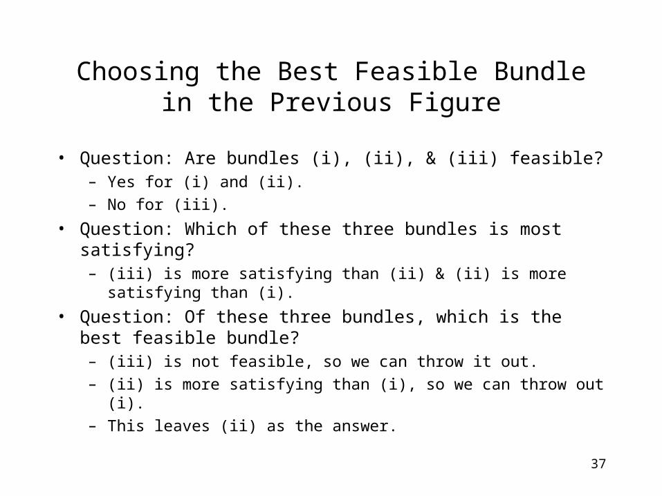
Choosing the Best Feasible Bundle in the Previous Figure

• Question: Are bundles (i), (ii), & (iii) feasible?– Yes for (i) and (ii).

– No for (iii).

• Question: Which of these three bundles is most satisfying?– (iii) is more satisfying than (ii) & (ii) is more satisfying than (i).

• Question: Of these three bundles, which is the best feasible bundle?– (iii) is not feasible, so we can throw it out.

– (ii) is more satisfying than (i), so we can throw out (i).

– This leaves (ii) as the answer.

38

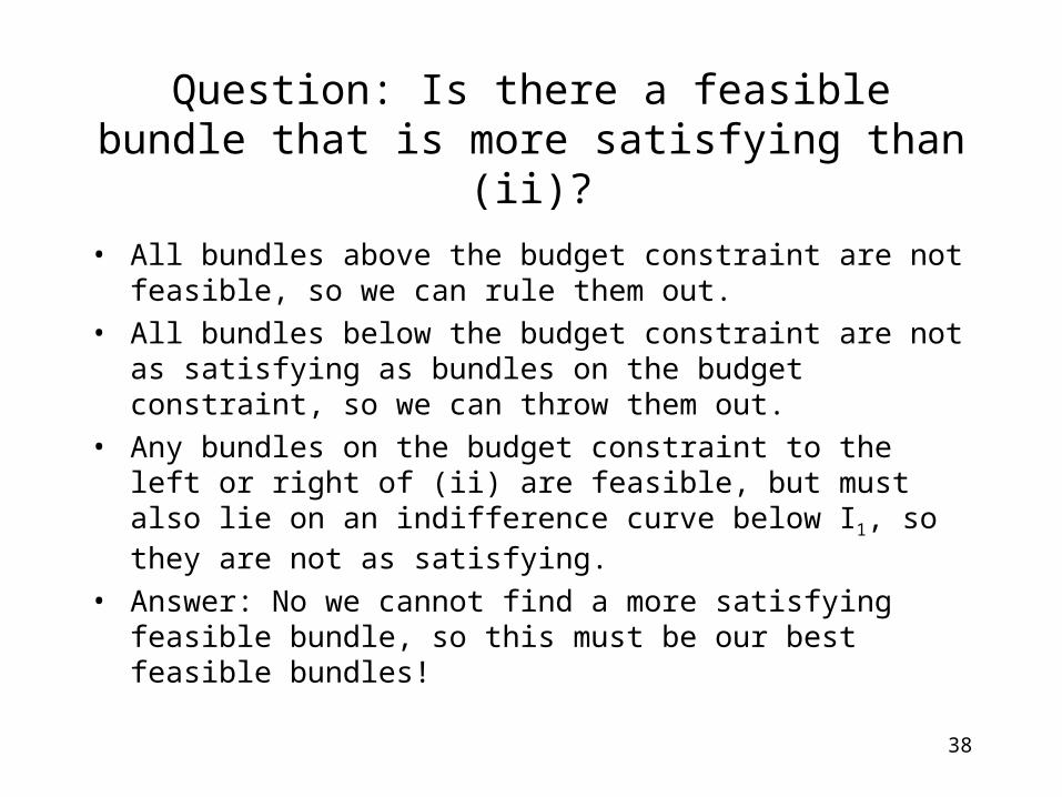
Question: Is there a feasible bundle that is more satisfying than (ii)?

• All bundles above the budget constraint are not feasible, so we can rule them out.

• All bundles below the budget constraint are not as satisfying as bundles on the budget constraint, so we can throw them out.

• Any bundles on the budget constraint to the left or right of (ii) are feasible, but must also lie on an indifference curve below I1, so they are not as satisfying.

• Answer: No we cannot find a more satisfying feasible bundle, so this must be our best feasible bundles!

39

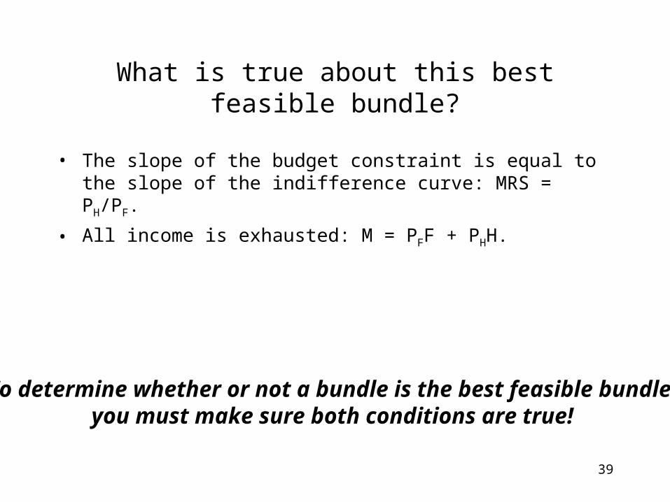
What is true about this best feasible bundle?

• The slope of the budget constraint is equal to the slope of the indifference curve: MRS = PH/PF.

• All income is exhausted: M = PFF + PHH.

To determine whether or not a bundle is the best feasible bundle,you must make sure both conditions are true!

40

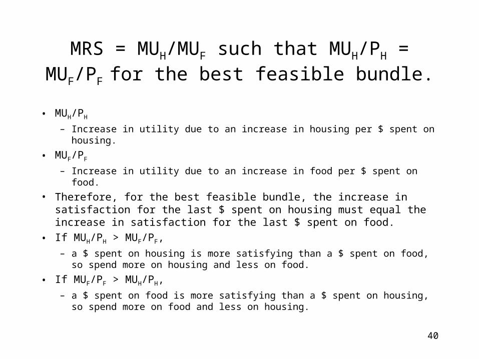
MRS = MUH/MUF such that MUH/PH = MUF/PF for the best feasible bundle.

• MUH/PH

– Increase in utility due to an increase in housing per $ spent on housing.

• MUF/PF

– Increase in utility due to an increase in food per $ spent on food.

• Therefore, for the best feasible bundle, the increase in satisfaction for the last $ spent on housing must equal the increase in satisfaction for the last $ spent on food.

• If MUH/PH > MUF/PF,

– a $ spent on housing is more satisfying than a $ spent on food, so spend more on housing and less on food.

• If MUF/PF > MUH/PH,

– a $ spent on food is more satisfying than a $ spent on housing, so spend more on food and less on housing.

41

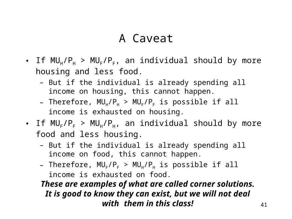
A Caveat

• If MUH/PH > MUF/PF, an individual should by more housing and less food.– But if the individual is already spending all income on housing, this

cannot happen.

– Therefore, MUH/PH > MUF/PF is possible if all income is exhausted on housing.

• If MUF/PF > MUH/PH, an individual should by more food and less housing.– But if the individual is already spending all income on food, this cannot

happen.

– Therefore, MUF/PF > MUH/PH is possible if all income is exhausted on food.

These are examples of what are called corner solutions.It is good to know they can exist, but we will not deal

with them in this class!

42

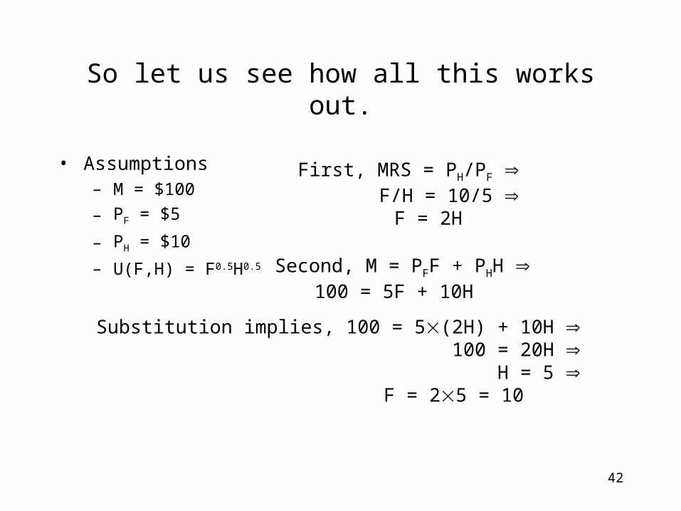
So let us see how all this works out.

• Assumptions– M = $100

– PF = $5

– PH = $10

– U(F,H) = F0.5H0.5

First, MRS = PH/PF F/H = 10/5

F = 2H

Second, M = PFF + PHH 100 = 5F + 10H

Substitution implies, 100 = 5(2H) + 10H 100 = 20H

H = 5 F = 25 = 10

43

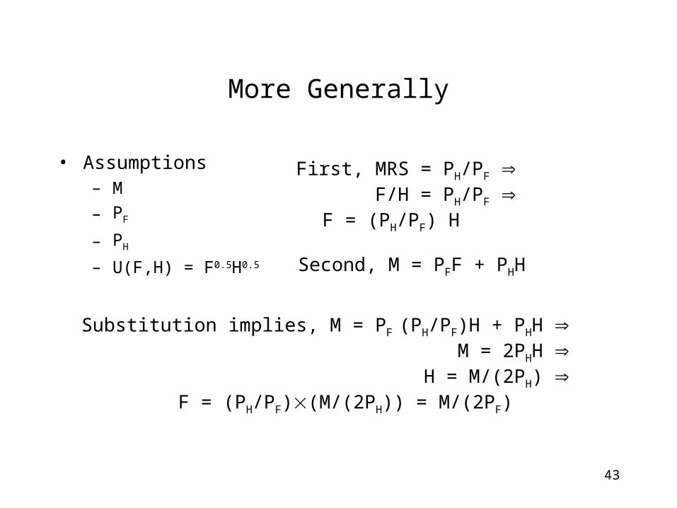
More Generally

• Assumptions– M

– PF

– PH

– U(F,H) = F0.5H0.5

First, MRS = PH/PF F/H = PH/PF

F = (PH/PF) H

Second, M = PFF + PHH

Substitution implies, M = PF (PH/PF)H + PHH M = 2PHH

H = M/(2PH) F = (PH/PF)(M/(2PH)) = M/(2PF)

44

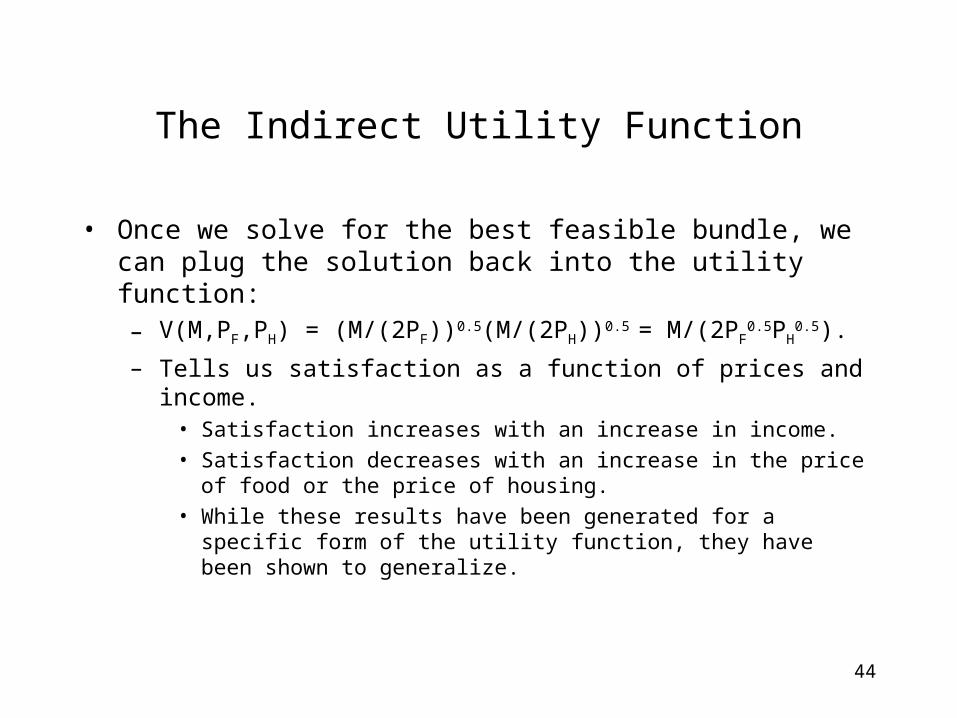
The Indirect Utility Function

• Once we solve for the best feasible bundle, we can plug the solution back into the utility function:– V(M,PF,PH) = (M/(2PF))0.5(M/(2PH))0.5

= M/(2PF0.5PH

0.5).

– Tells us satisfaction as a function of prices and income.• Satisfaction increases with an increase in income.

• Satisfaction decreases with an increase in the price of food or the price of housing.

• While these results have been generated for a specific form of the utility function, they have been shown to generalize.

45

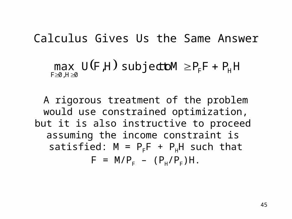
Calculus Gives Us the Same Answer

HPFPMtosubjectHF,Umax HF0H0,F

A rigorous treatment of the problemwould use constrained optimization,but it is also instructive to proceed assuming the income constraint is satisfied: M = PFF + PHH such that

F = M/PF – (PH/PF)H.

46

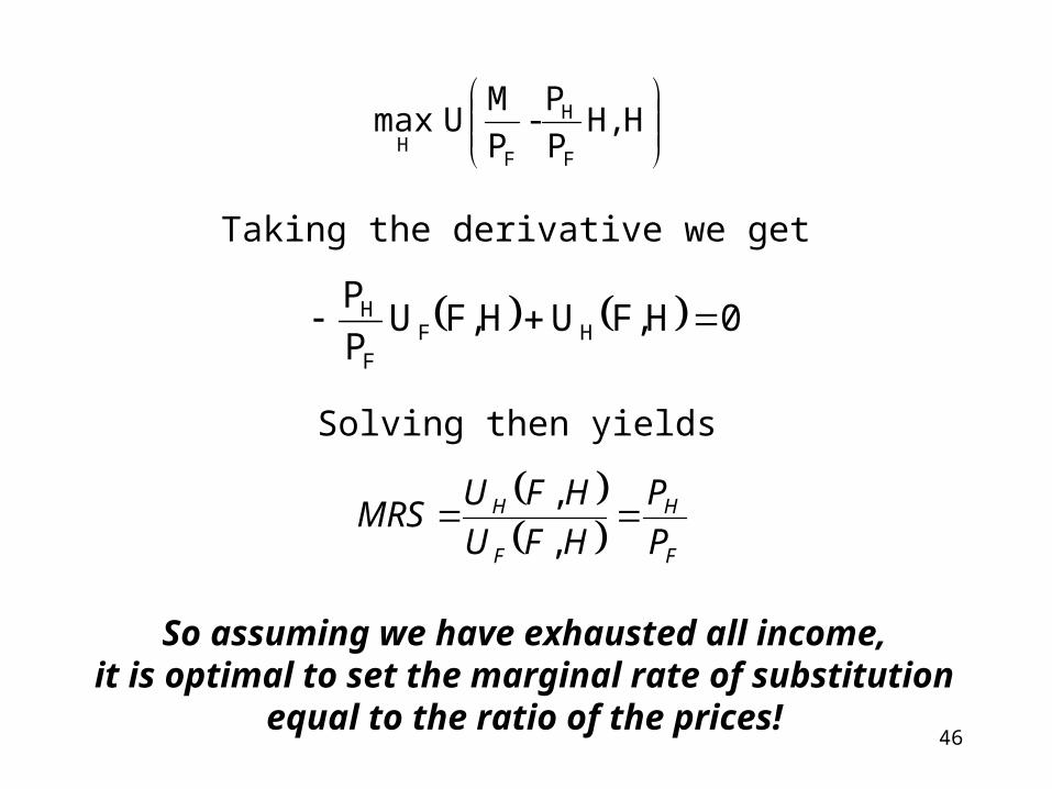
HH,

P

P-

P

MUmax

F

H

FH

0HF,UHF,UP

PHF

F

H

Taking the derivative we get

Solving then yields

F

H

F

H

P

P

HFU

HFUMRS

,

,

So assuming we have exhausted all income,it is optimal to set the marginal rate of substitution

equal to the ratio of the prices!

47

What Should You Know

• How budgets constraint describes limited means.

• The relationship between the budget constraint, prices, & income.

• How indifference curves & the utility function describe unlimited wants.

• How indifference curves & the utility function can be used with the budget constraint to determine an individual’s best feasible consumption bundle.