Embed Size (px)
Citation preview
1
Queuing Models
Dr. Mahmoud Alrefaei
2
Introduction
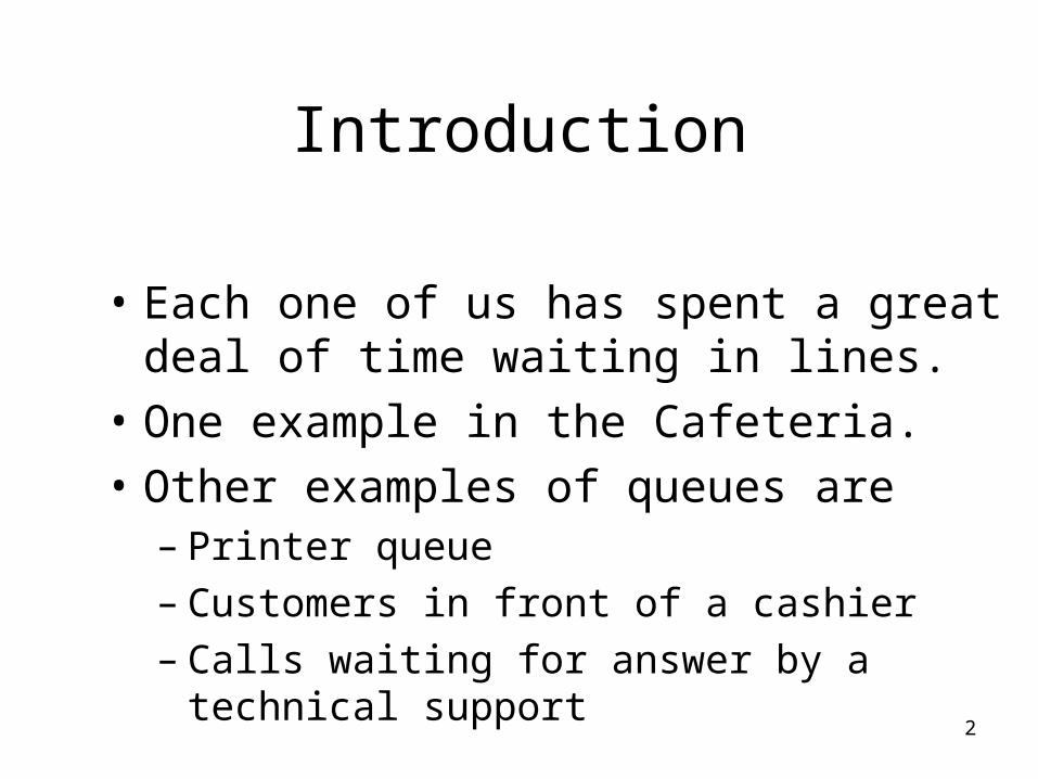
• Each one of us has spent a great deal of time waiting in lines.
• One example in the Cafeteria.
• Other examples of queues are– Printer queue– Customers in front of a cashier – Calls waiting for answer by a technical support
3
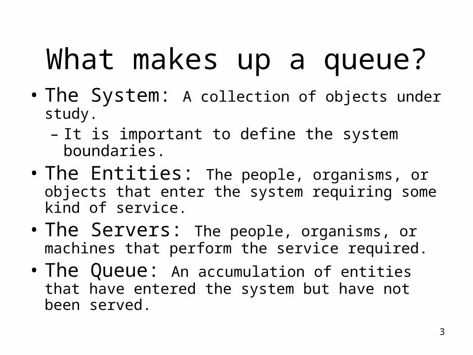
What makes up a queue?• The System: A collection of objects under study.
– It is important to define the system boundaries.
• The Entities: The people, organisms, or objects that enter the system requiring some kind of service.
• The Servers: The people, organisms, or machines that perform the service required.
• The Queue: An accumulation of entities that have entered the system but have not been served.
4
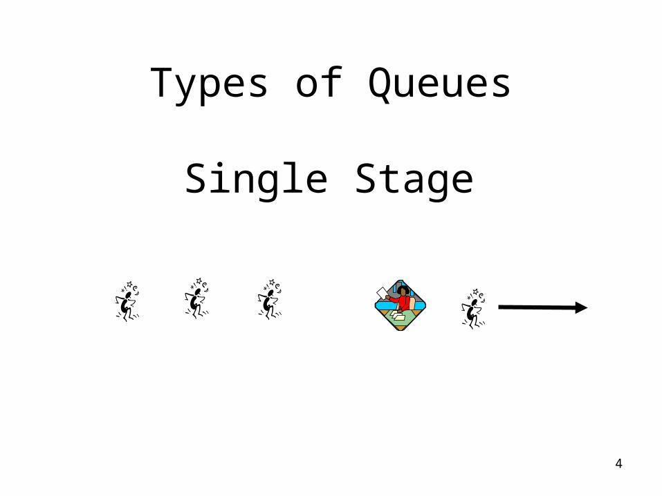
Types of Queues
Single Stage

5
Multiple Stage - Manufacturing Plant
6
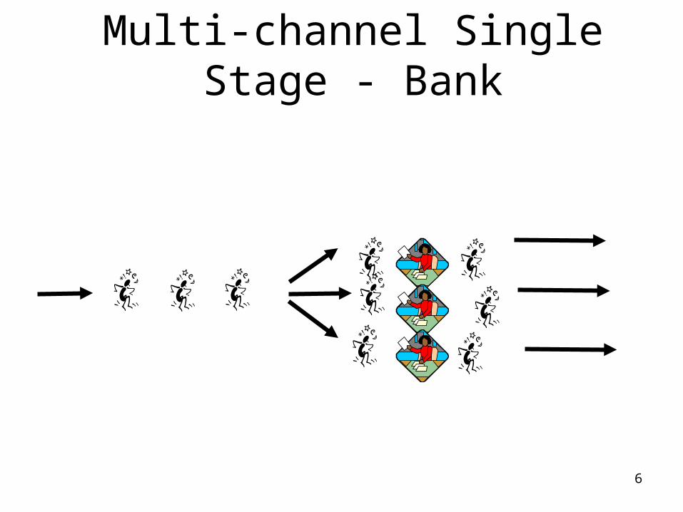
Multi-channel Single Stage - Bank
7
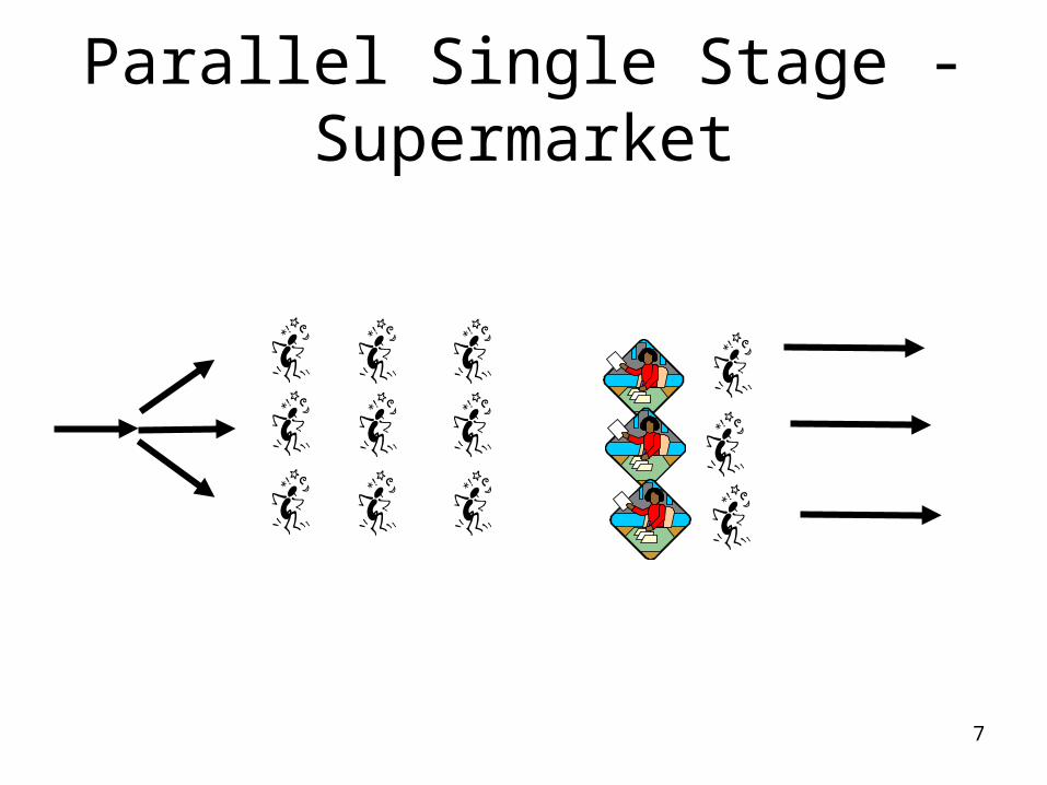
Parallel Single Stage - Supermarket
8
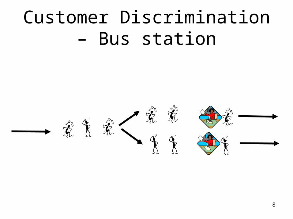
Customer Discrimination – Bus station
9
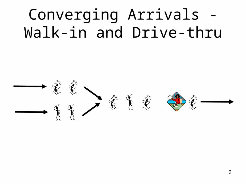
Converging Arrivals - Walk-in and Drive-thru
10
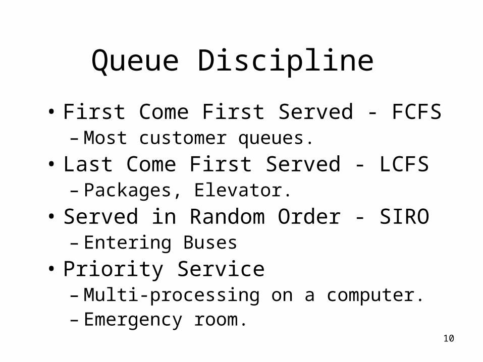
Queue Discipline
• First Come First Served - FCFS– Most customer queues.
• Last Come First Served - LCFS– Packages, Elevator.
• Served in Random Order - SIRO– Entering Buses
• Priority Service– Multi-processing on a computer.– Emergency room.
11
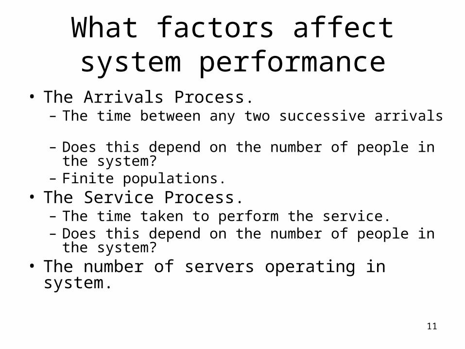
What factors affect system performance
• The Arrivals Process.– The time between any two successive arrivals – Does this depend on the number of people in the
system?– Finite populations.
• The Service Process.– The time taken to perform the service.– Does this depend on the number of people in the
system?• The number of servers operating in system.
12
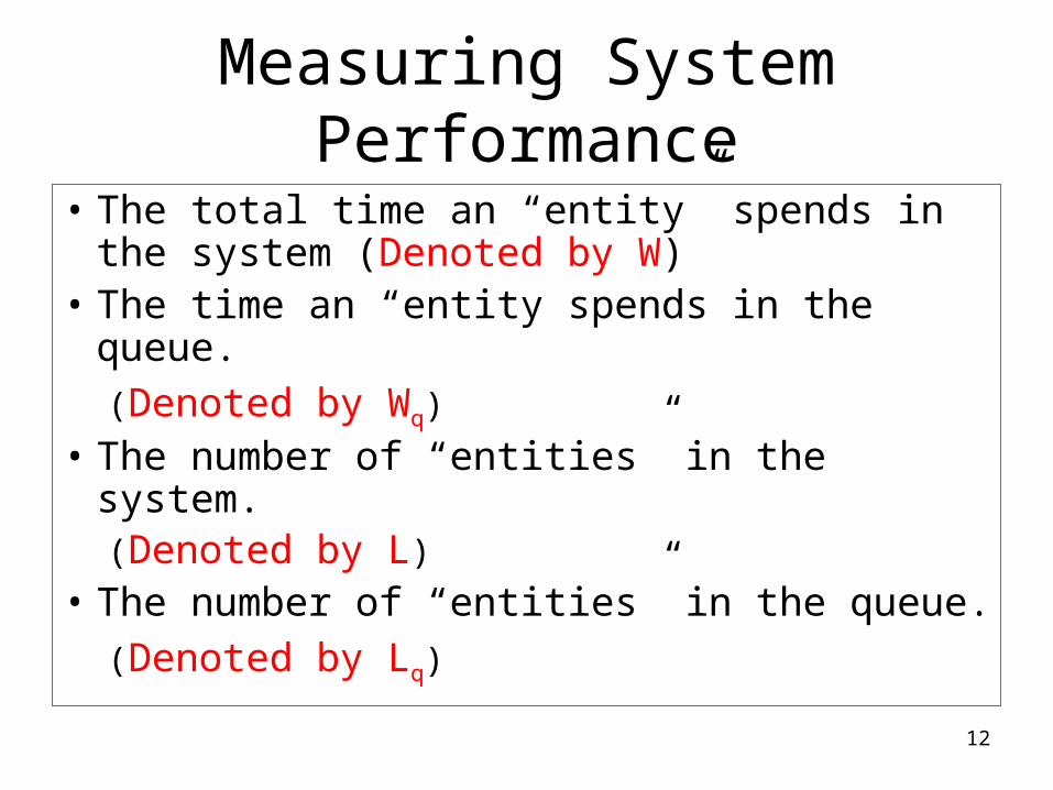
Measuring System Performance
• The total time an “entity” spends in the system (Denoted by W)
• The time an “entity spends in the queue.
(Denoted by Wq)
• The number of “entities” in the system.(Denoted by L)
• The number of “entities” in the queue.
(Denoted by Lq)
13
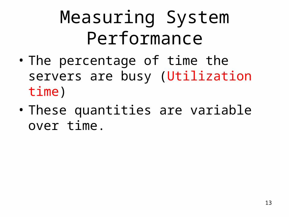
Measuring System Performance
• The percentage of time the servers are busy (Utilization time)
• These quantities are variable over time.
14
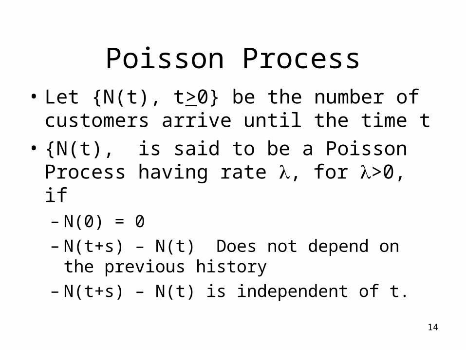
Poisson Process• Let {N(t), t>0} be the number of customers
arrive until the time t
• {N(t), is said to be a Poisson Process having rate , for >0, if– N(0) = 0– N(t+s) – N(t) Does not depend on the
previous history– N(t+s) – N(t) is independent of t.
15
Poisson Process
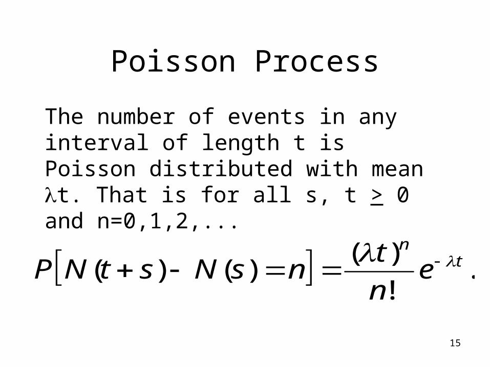
The number of events in any interval of length t is Poisson distributed with mean t. That is for all s, t > 0 and n=0,1,2,...
.!
)()()( t
n
en
tnsNstNP
16
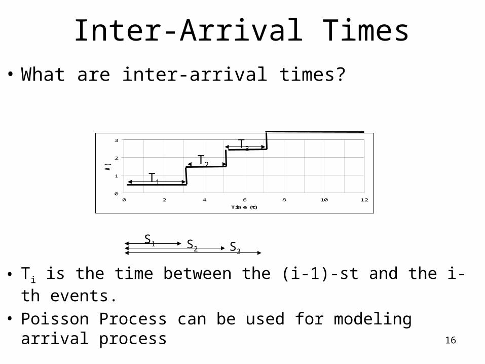
Inter-Arrival Times
• What are inter-arrival times?
• Ti is the time between the (i-1)-st and the i-th events.
• Poisson Process can be used for modeling arrival process
0
1
2
3
0 2 4 6 8 10 12
Time (t)
A(t)
T1
T2
T3
S1 S2 S3
17
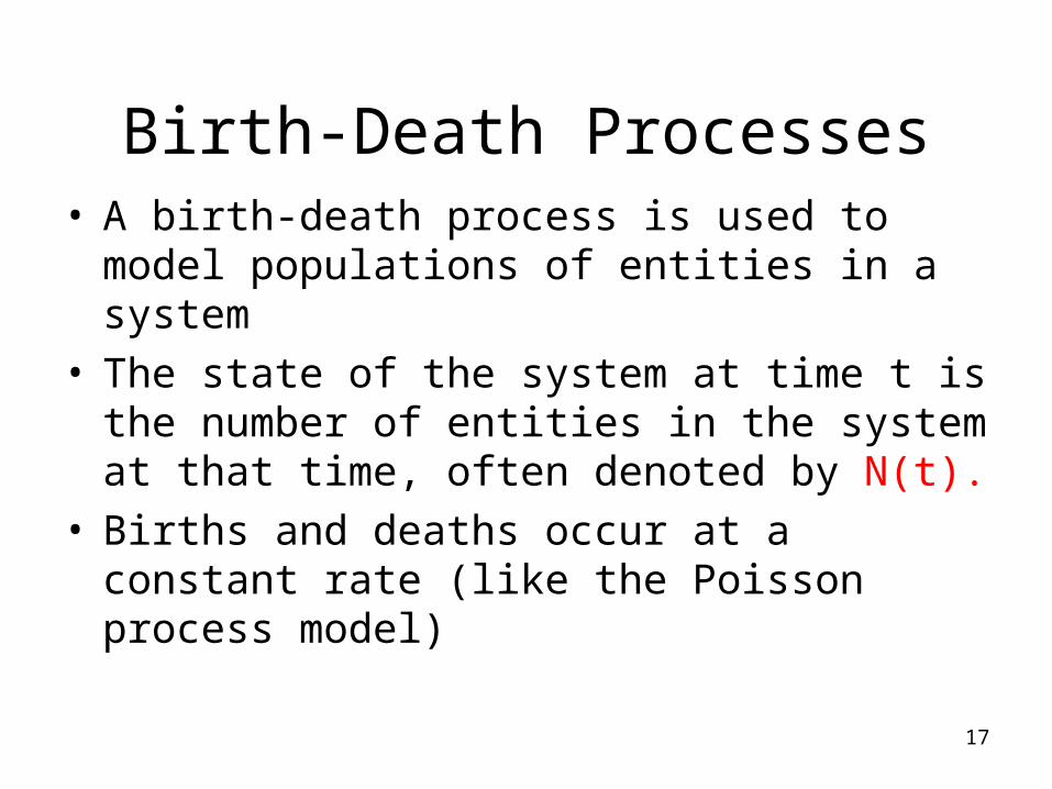
Birth-Death Processes• A birth-death process is used to model
populations of entities in a system• The state of the system at time t is the number
of entities in the system at that time, often denoted by N(t).
• Births and deaths occur at a constant rate (like the Poisson process model)
18
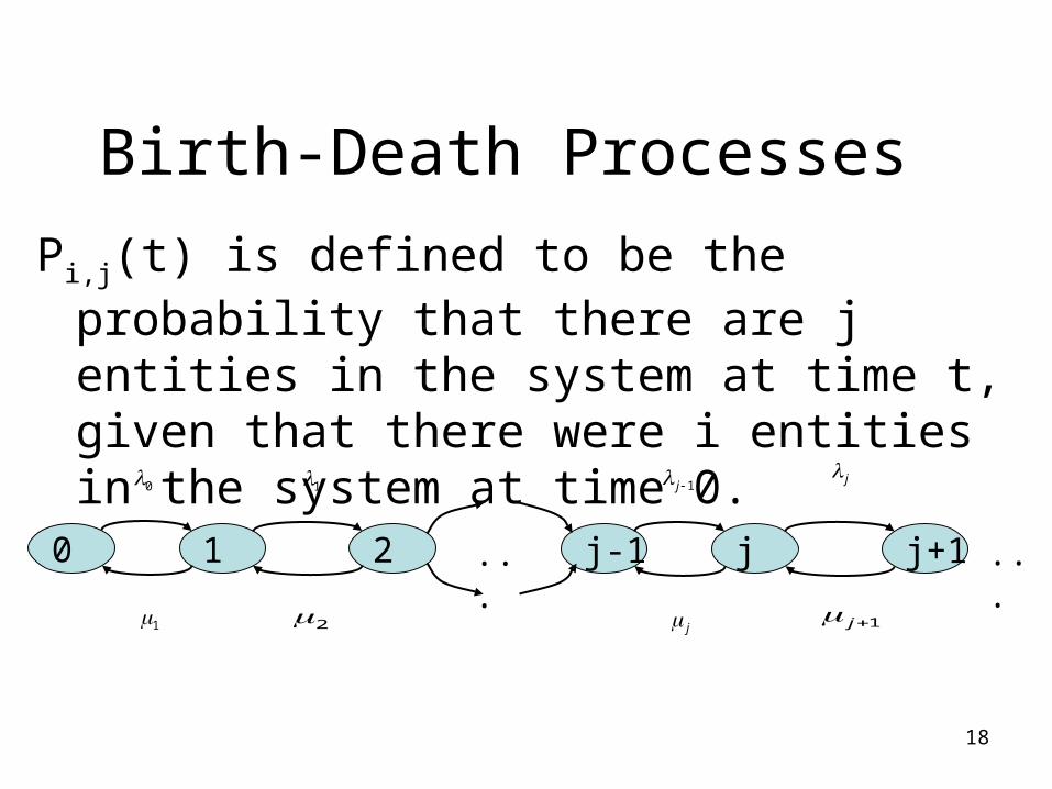
Birth-Death Processes
Pi,j(t) is defined to be the probability that there are j entities in the system at time t, given that there were i entities in the system at time 0.
0 1 2 j-1 j j+1
0 1 1j j
1 2j 1j
... ...
19
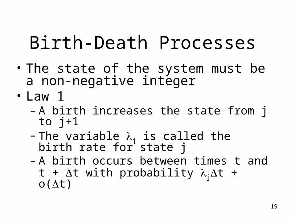
Birth-Death Processes• The state of the system must be a non-
negative integer• Law 1
– A birth increases the state from j to j+1– The variable j is called the birth rate for
state j– A birth occurs between times t and t + t with
probability jt + o(t)
20
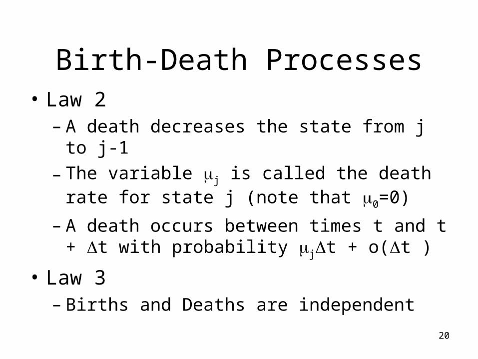
Birth-Death Processes• Law 2
– A death decreases the state from j to j-1
– The variable j is called the death rate for state j (note that 0=0)
– A death occurs between times t and t + t with probability jt + o(t )
• Law 3– Births and Deaths are independent
21
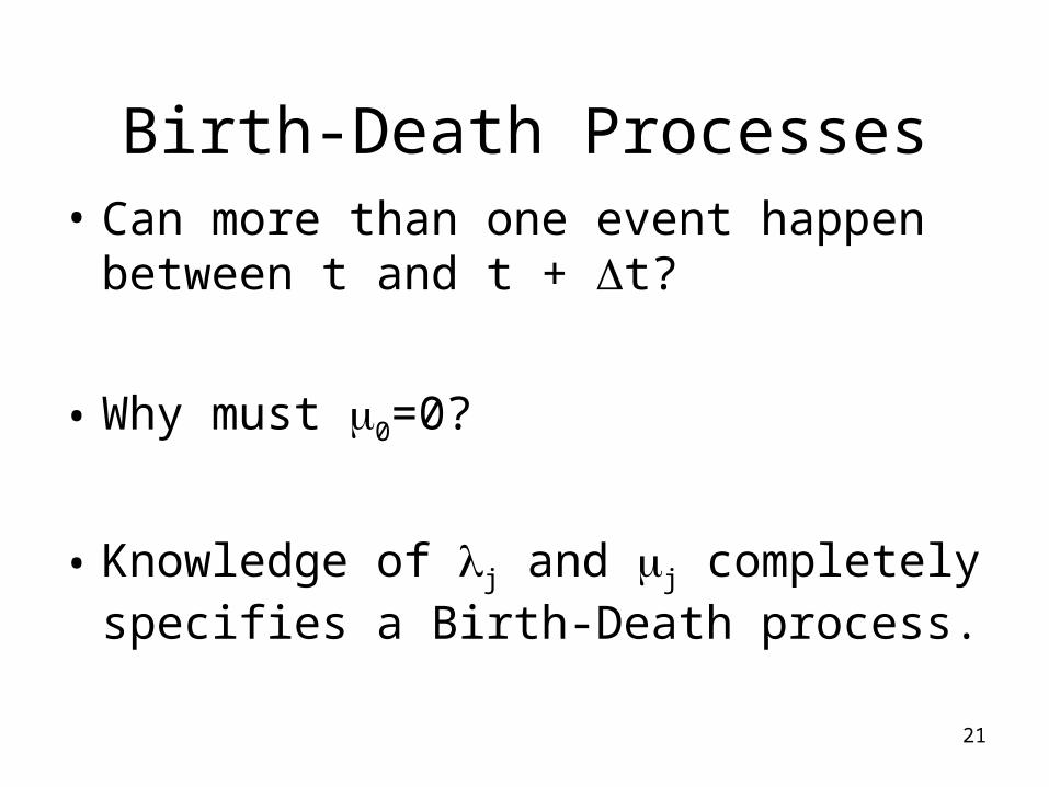
Birth-Death Processes• Can more than one event happen between
t and t + t?
• Why must 0=0?
• Knowledge of j and j completely specifies a Birth-Death process.
22
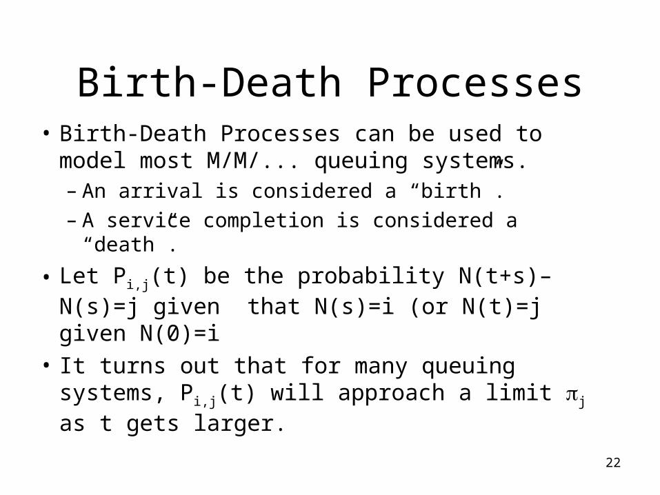
Birth-Death Processes• Birth-Death Processes can be used to
model most M/M/... queuing systems.– An arrival is considered a “birth”.– A service completion is considered a “death”.
• Let Pi,j(t) be the probability N(t+s)–N(s)=j given that N(s)=i (or N(t)=j given N(0)=i
• It turns out that for many queuing systems, Pi,j(t) will approach a limit j as t gets larger.
23
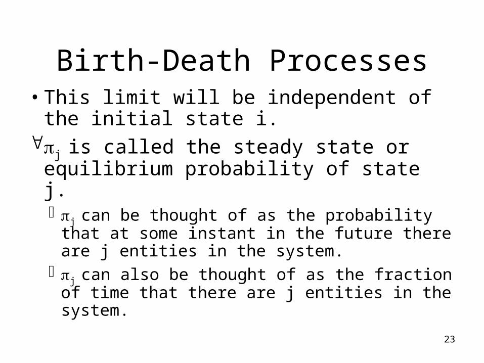
Birth-Death Processes• This limit will be independent of the
initial state i.j is called the steady state or
equilibrium probability of state j. j can be thought of as the probability that
at some instant in the future there are j entities in the system.
j can also be thought of as the fraction of time that there are j entities in the system.
24
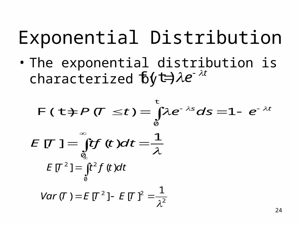
Exponential Distribution• The exponential distribution is
characterized by
1)(][
1)(F(t)
0
t
0
dtttfTE
edsetTP ts
222
0
22
1][][)(
)(][
TETETVar
dttftTE
te f(t)
25
Exponential Distribution
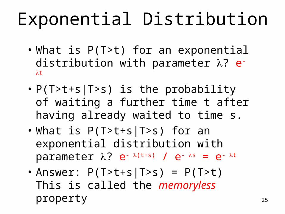
• What is P(T>t) for an exponential distribution with parameter ? e- t
• P(T>t+s|T>s) is the probability of waiting a further time t after having already waited to time s.
• What is P(T>t+s|T>s) for an exponential distribution with parameter ? e- (t+s) / e- s = e- t
• Answer: P(T>t+s|T>s) = P(T>t) This is called the memoryless property
26
An Example of Memoryless
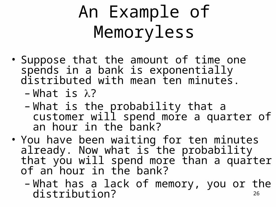
• Suppose that the amount of time one spends in a bank is exponentially distributed with mean ten minutes.– What is ?– What is the probability that a customer will spend
more a quarter of an hour in the bank?• You have been waiting for ten minutes already. Now
what is the probability that you will spend more than a quarter of an hour in the bank?– What has a lack of memory, you or the
distribution?
27
Birth-Death Processes
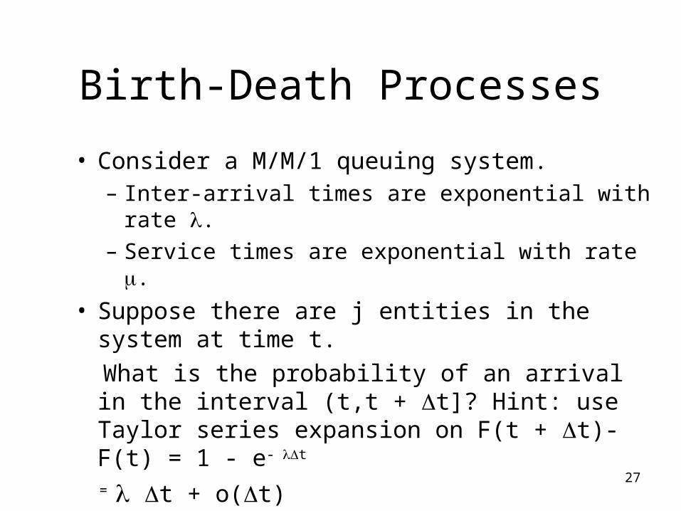
• Consider a M/M/1 queuing system.– Inter-arrival times are exponential with rate .
– Service times are exponential with rate .
• Suppose there are j entities in the system at time t.
What is the probability of an arrival in the interval (t,t + t]? Hint: use Taylor series expansion on F(t + t)-F(t) = 1 - e- t
= t + o(t)
28
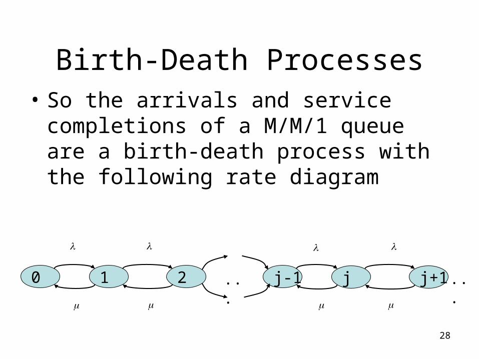
Birth-Death Processes• So the arrivals and service completions of
a M/M/1 queue are a birth-death process with the following rate diagram
0 1 2 j-1 j j+1
... ...
29
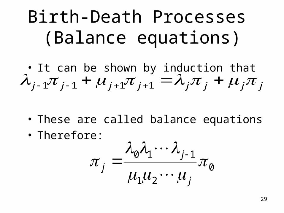
Birth-Death Processes (Balance equations)
• It can be shown by induction that
• These are called balance equations• Therefore:
jjjjjjjj 1111
021
110
j
jj
30
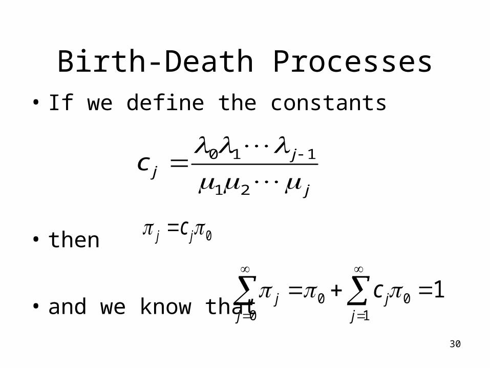
Birth-Death Processes• If we define the constants
• then
• and we know that
j
jjc
21
110
0 jj c
11
000
jj
jj c
31
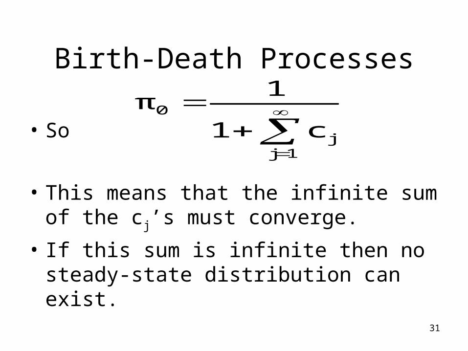
Birth-Death Processes
• So
• This means that the infinite sum of the cj’s must converge.
• If this sum is infinite then no steady-state distribution can exist.
1jj
0
c1
1π