PARAMETER ESTIMATION FOR MULTIVARIATE EXPONENTIALSUMS

DANIEL POTTS∗ AND MANFRED TASCHE‡

Abstract. The recovery of signal parameters from noisy sampled data is an essential problem indigital signal processing. In this paper, we discuss the numerical solution of the following parameterestimation problem. Let h0 be a multivariate exponential sum, i.e., h0 is a finite linear combinationof complex exponentials with distinct frequency vectors. Determine all parameters of h0, i.e., allfrequency vectors, all coefficients, and the number of exponentials, if finitely many sampled dataof h0 are given. Using Ingham–type inequalities, the Riesz stability of finitely many multivariateexponentials with well–separated frequency vectors is discussed in continuous as well as discretenorms. Further we show that a rectangular Fourier–type matrix has a bounded condition number,if the frequency vectors are well–separated and if the number of samples is sufficiently large. Thenwe reconstruct the parameters of an exponential sum h0 by a novel algorithm, the so–called sparseapproximate Prony method (SAPM), where we use only some data sampled along few straight lines.The first part of SAPM estimates the frequency vectors by using the approximate Prony method inthe univariate case. The second part of SAPM computes all coefficients by solving an overdeterminedlinear Vandermonde–type system. Numerical experiments show the performance of our method.

Key words and phrases: Parameter estimation, multivariate exponential sum, multivariate expo-nential fitting problem, harmonic retrieval, sparse approximate Prony method, sparse approximaterepresentation of signals.

AMS Subject Classifications: 65D10, 65T40, 41A45, 41A63, 65F20, 94A12.

1. Introduction. Let the dimension d ∈ N and a positive integer M ∈ N\{1} begiven. We consider a d-variate exponential sum of order M that is a linear combination

h0(x) :=

M∑j=1

cj eifj ·x (x = (xl)dl=1 ∈ Rd) (1.1)

of M complex exponentials with complex coefficients cj 6= 0 and distinct frequencyvectors f j = (fj,l)

dl=1 ∈ Td ∼= [−π, π)d. Assume that |cj | > ε0 (j = 1, . . . ,M) for a

convenient bound 0 < ε0 � 1. Here the torus T is identified with the interval [−π, π).Further the dots in the exponents of (1.1) denote the usual scalar product in Rd.If h0 is real–valued, then (1.1) can be represented as a linear combination of ridgefunctions

h0(x) =

M∑j=1

|cj | cos(f j · x+ ϕj

)with cj = |cj | eiϕj . Assume that the frequency vectors f j ∈ Td (j = 1, . . . ,M) fulfill

the gap condition on Td

dist(f j ,f l) := min{‖(f j + 2πk)− f l‖∞ : k ∈ Zd} ≥ q > 0 (1.2)

for all j, l = 1, . . . ,M with j 6= l. Let N ∈ N with N ≥ 2M + 1 be given. In thefollowing G is either the full grid ZdN := [−N,N ]d ∩ Zd or a union of 2N + 1 gridpoints n ∈ Zd lying on few straight lines. If G is chosen such that |G| � (2N + 1)d

∗potts@mathematik.tu-chemnitz.de, Chemnitz University of Technology, Faculty of Mathemat-ics, D–09107 Chemnitz, Germany‡manfred.tasche@uni-rostock.de, University of Rostock, Institute of Mathematics, D–18051 Ro-

stock, Germany

1

for d ≥ 2, then G is called a sparse sampling grid.Suppose that perturbed sampled data

h(n) := h0(n) + e(n), |e(n)| ≤ ε

of (1.1) for all n ∈ G are given, where the error terms e(n) ∈ C are bounded by certainaccuracy ε > 0. Then we consider the following parameter estimation problem for thed–variate exponential sum (1.1): Recover the distinct frequency vectors f j ∈ [−π, π)d

and the complex coefficients cj so that

|h(n)−M∑j=1

cj eifj ·n| ≤ ε (n ∈ G) (1.3)

for very small accuracy ε > 0 and for minimal order M . In other words, we areinterested in sparse approximate representations of the given noisy data h(n) ∈ C(n ∈ G) by sampled data of the exponential sum (1.1), where the condition (1.3) isfulfilled.The approximation of data by finite linear combinations of complex exponentials hasa long history, see [19, 20]. There exists a variety of applications, such as fittingnuclear magnetic resonance spectroscopic data [18] or the annihilating filter method[31, 6, 30]. Recently, the reconstruction method of [3] was generalized to bivariateexponential sums in [1]. In contrast to [1], we introduce a sparse approximate Pronymethod, where we use only some data on a sparse sampling grid G. Further weremark the relation to a reconstruction method for sparse multivariate trigonometricpolynomials, see Remark 6.3 and [14, 12, 32].

In this paper, we extend the approximate Prony method (see [23]) to multivariateexponential sums. Our approach can be described as follows:(i) Solving a few reconstruction problems of univariate exponential sums, we determinea finite set of feasible frequency vectors f ′k (k = 1, . . . ,M ′). For each reconstructionwe use only data sampled along a straight line. As parameter estimation we usethe univariate approximate Prony method which can be replaced by another Prony–like method [24], such as ESPRIT (Estimation of Signal Parameters via RotationalInvariance Techniques) [26, 27] or matrix pencil methods [10, 29].(ii) Then we test, if a feasible frequency vector f ′k (k = 1, . . . ,M ′) is an actualfrequency vector of the exponential sum (1.1) too. Replacing the condition (1.3) bythe overdetermined linear system

M ′∑k=1

c′k eif′k·n = h(n) (n ∈ G) , (1.4)

we compute the least squares solution (c′k)M′

k=1. Then we say that f ′k is an actualfrequency vector of (1.1), if |c′k| > ε0. Otherwise, f ′k is interpreted as frequency

vector of noise and is canceled. Let f j (j = 1, . . . ,M) be all the actual frequencyvectors.(iii) In a final correction step, we solve the linear system

M∑j=1

cj eifj ·n = h(n) (n ∈ G) .

2

As explained above, our reconstruction method uses the least squares solution of thelinear system (1.4) with the rectangular coefficient matrix(

eifj ·n)n∈G, j=1,...,M

(|G| > M) .

If this matrix has full rank M and if its condition number is moderately sized, thenone can efficiently compute the least squares solution of (1.4), which is sensitive topermutations of the coefficient matrix and the sampled data (see [7, pp. 239 – 244]).In the special case G = ZdN , we can show that this matrix is uniformly bounded, if

N >√dπq . Then we use (2N+1)d sampled data for the reconstruction of M frequency

vectors f j and M complex coefficients cj of (1.1).But our aim is an efficient parameter estimation of (1.1) by a relatively low numberof given sampled data h(n) (n ∈ G) on a sparse sampling grid G. The correspondingapproach is called sparse approximate Prony method (SAPM). Numerical experimentsfor d–variate exponential sums with d ∈ {2, 3, 4} show the performance of our pa-rameter reconstruction.

This paper is divided into two parts. The first part consists of Sections 2 and 3,where we discuss the Riesz stability of finitely many multivariate exponentials. It is aknown fact that an exponential sum (1.1) with well–separated frequency vectors canbe well reconstructed. Otherwise, one also knows that the parameter estimation of anexponential sum with clustered frequency vectors is very difficult. What is the basiccause of these effects? In Section 2, we investigate the Riesz stability of multivariateexponentials with respect to the continuous norms of L2([−N, N ]d) and C([−N, N ]d),respectively, where we assume that the frequency vectors fulfill the gap condition (2.1)(see Lemma 2.1 and Corollary 2.3). These results are mainly based on Ingham–typeinequalities (see [15, pp. 59 – 66 and pp. 153 – 156]). Furthermore we present a resultfor the converse assertion, i.e., if finitely many multivariate exponentials are Rieszstable, then the corresponding frequency vectors are well–separated (see Lemma 2.2).In Section 3, we extend these stability results to draw conclusions for the discretenorm of `2(ZdN ). Further we prove that the condition number of the coefficient matrixof (1.4) is uniformly bounded, if we choose the full sampling grid G = ZdN and ifN is sufficiently large. By the results of Section 3, one can see that well–separatedfrequency vectors are essential for a successful parameter estimation of (1.1). Up tonow, a corresponding result for a sparse sampling grid G is unknown.The second part of this paper consists of Sections 4 – 7, where we present a novelefficient parameter recovery algorithm of (1.1) for a sparse sampling grid. In Section4 we sketch the approximate Prony method in the univariate setting. Then we extendthis method to bivariate exponential sums in Section 5. Here we suggest the newSAPM. The main idea is to project the bivariate reconstruction problem to severalunivariate problems and combine finally the results of the univariate reconstructions.We use only few data sampled along some straight lines in order to reconstruct abivariate exponential sum. In Section 6, we extend this reconstruction method tod–variate exponential sums for moderately sized dimensions d ≥ 3. Finally, variousnumerical examples are presented in Section 7.

2. Stability of exponentials. As known, the main difficulty is the reconstruc-tion of frequency vectors with small separation distance q > 0 (see (1.2)). Thereforefirst we discuss the stability properties of the finitely many d–variate exponentials independence of q. We start with a generalization of the known Ingham inequalities(see [11]):

3

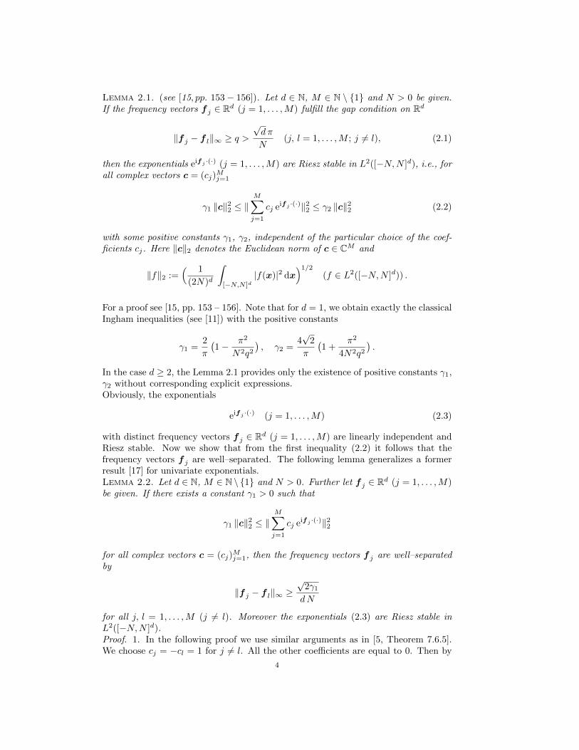
Lemma 2.1. (see [15, pp. 153− 156]). Let d ∈ N, M ∈ N \ {1} and N > 0 be given.If the frequency vectors f j ∈ Rd (j = 1, . . . ,M) fulfill the gap condition on Rd

‖f j − f l‖∞ ≥ q >√d π

N(j, l = 1, . . . ,M ; j 6= l), (2.1)

then the exponentials eifj ·(·) (j = 1, . . . ,M) are Riesz stable in L2([−N,N ]d), i.e., forall complex vectors c = (cj)

Mj=1

γ1 ‖c‖22 ≤ ‖M∑j=1

cj eifj ·(·)‖22 ≤ γ2 ‖c‖22 (2.2)

with some positive constants γ1, γ2, independent of the particular choice of the coef-ficients cj. Here ‖c‖2 denotes the Euclidean norm of c ∈ CM and

‖f‖2 :=( 1

(2N)d

∫[−N,N ]d

|f(x)|2 dx)1/2

(f ∈ L2([−N,N ]d)) .

For a proof see [15, pp. 153 – 156]. Note that for d = 1, we obtain exactly the classicalIngham inequalities (see [11]) with the positive constants

γ1 =2

π

(1− π2

N2q2), γ2 =

4√

2

π

(1 +

π2

4N2q2).

In the case d ≥ 2, the Lemma 2.1 provides only the existence of positive constants γ1,γ2 without corresponding explicit expressions.Obviously, the exponentials

eifj ·(·) (j = 1, . . . ,M) (2.3)

with distinct frequency vectors f j ∈ Rd (j = 1, . . . ,M) are linearly independent andRiesz stable. Now we show that from the first inequality (2.2) it follows that thefrequency vectors f j are well–separated. The following lemma generalizes a formerresult [17] for univariate exponentials.Lemma 2.2. Let d ∈ N, M ∈ N \ {1} and N > 0. Further let f j ∈ Rd (j = 1, . . . ,M)be given. If there exists a constant γ1 > 0 such that

γ1 ‖c‖22 ≤ ‖M∑j=1

cj eifj ·(·)‖22

for all complex vectors c = (cj)Mj=1, then the frequency vectors f j are well–separated

by

‖f j − f l‖∞ ≥√

2γ1dN

for all j, l = 1, . . . ,M (j 6= l). Moreover the exponentials (2.3) are Riesz stable inL2([−N,N ]d).Proof. 1. In the following proof we use similar arguments as in [5, Theorem 7.6.5].We choose cj = −cl = 1 for j 6= l. All the other coefficients are equal to 0. Then by

4

the assumption, we obtain

2 γ1 ≤ ‖eifj ·(·) − eif l·(·)‖22

=1

(2N)d

∫[−N,N ]d

|1− ei(f l−fj)·x|2 dx

=1

(2N)d

∫[−N,N ]d

4 sin2((f l − f j) · x/2

)dx

≤ 1

(2N)d

∫[−N,N ]d

∣∣(f l − f j) · x∣∣2 dx

≤ 1

(2N)d

∫[−N,N ]d

‖f l − f j‖21N2 dx , (2.4)

where we have used the Holder estimate

|(f l − f j) · x| ≤ ‖f l − f j‖1 ‖x‖∞ ≤ ‖f l − f j‖1N

for all x ∈ [−N, N ]d. Therefore (2.4) shows that

d ‖f l − f j‖∞ ≥ ‖f l − f j‖1 ≥√

2γ1N

for all j, l = 1, . . . ,M (j 6= l).2. We see immediately that M is an upper Riesz bound for the exponentials (2.3) inL2([−N,N ]d). By the Cauchy–Schwarz inequality we obtain

|M∑j=1

cj eifj ·x|2 ≤M ‖c‖22

for all c = (cj)Mj=1 ∈ CM and all x ∈ [−N, N ]d such that

‖M∑j=1

cj eifj ·(·)‖22 ≤M ‖c‖22 .

This completes the proof.

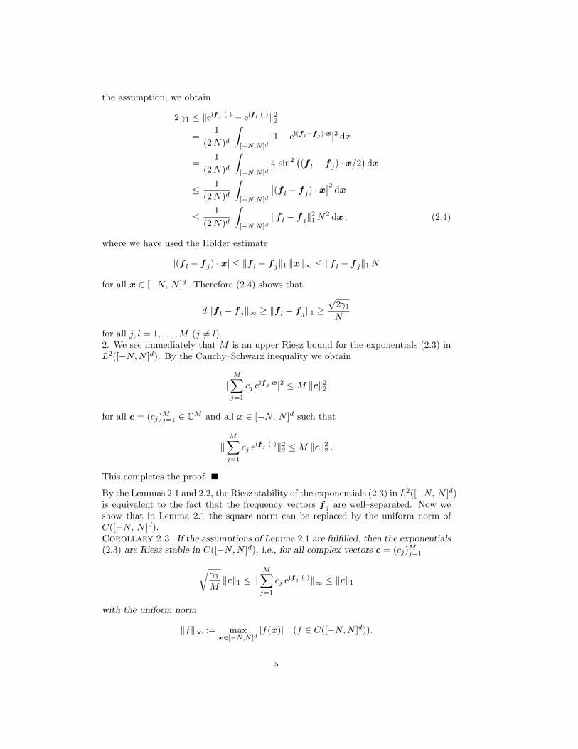
By the Lemmas 2.1 and 2.2, the Riesz stability of the exponentials (2.3) in L2([−N, N ]d)is equivalent to the fact that the frequency vectors f j are well–separated. Now weshow that in Lemma 2.1 the square norm can be replaced by the uniform norm ofC([−N, N ]d).Corollary 2.3. If the assumptions of Lemma 2.1 are fulfilled, then the exponentials(2.3) are Riesz stable in C([−N,N ]d), i.e., for all complex vectors c = (cj)

Mj=1√

γ1M‖c‖1 ≤ ‖

M∑j=1

cj eifj ·(·)‖∞ ≤ ‖c‖1

with the uniform norm

‖f‖∞ := maxx∈[−N,N ]d

|f(x)| (f ∈ C([−N,N ]d)).

5

Proof. Let h0 ∈ C([−N,N ]d) be defined by (1.1). Then ‖h0‖2 ≤ ‖h0‖∞ <∞. Usingthe triangle inequality, we obtain that

‖h0‖∞ ≤M∑j=1

|cj | · 1 = ‖c‖1 .

From Lemma 2.1 and ‖c‖1 ≤√M ‖c‖2, it follows that√

γ1M‖c‖1 ≤

√γ1 ‖c‖2 ≤ ‖h0‖2 .

This completes the proof.

Now we use the uniform norm of C([−N, N ]d) and estimate the error ‖h0 − h‖∞between the original exponential sum (1.1) and its reconstruction

h(x) :=M∑j=1

cj eifj ·x (x ∈ [−N, N ]d).

We obtain a small error ‖h0− h‖∞ in the case∑Mj=1 |cj − cj | � 1 and ‖f j − f j‖∞ ≤

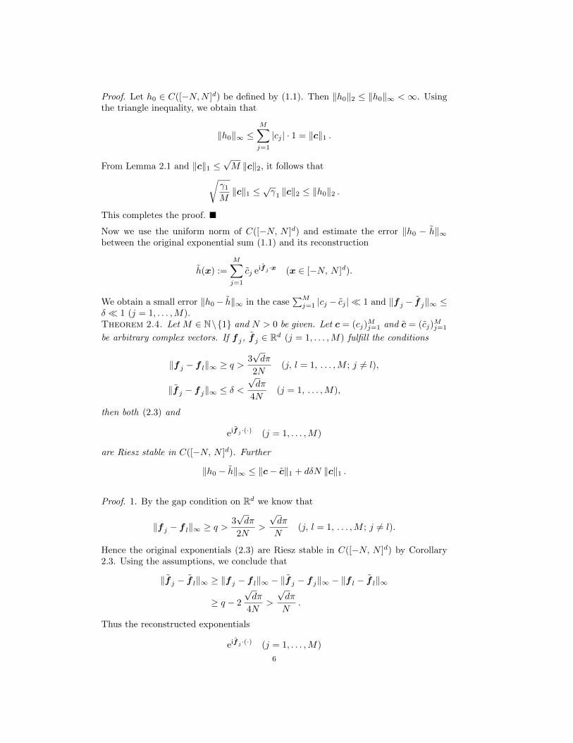
δ � 1 (j = 1, . . . ,M).Theorem 2.4. Let M ∈ N\{1} and N > 0 be given. Let c = (cj)

Mj=1 and c = (cj)

Mj=1

be arbitrary complex vectors. If f j, f j ∈ Rd (j = 1, . . . ,M) fulfill the conditions

‖f j − f l‖∞ ≥ q >3√dπ

2N(j, l = 1, . . . ,M ; j 6= l),

‖f j − f j‖∞ ≤ δ <√dπ

4N(j = 1, . . . ,M),

then both (2.3) and

eifj ·(·) (j = 1, . . . ,M)

are Riesz stable in C([−N, N ]d). Further

‖h0 − h‖∞ ≤ ‖c− c‖1 + dδN ‖c‖1 .

Proof. 1. By the gap condition on Rd we know that

‖f j − f l‖∞ ≥ q >3√dπ

2N>

√dπ

N(j, l = 1, . . . ,M ; j 6= l).

Hence the original exponentials (2.3) are Riesz stable in C([−N, N ]d) by Corollary2.3. Using the assumptions, we conclude that

‖f j − f l‖∞ ≥ ‖f j − f l‖∞ − ‖f j − f j‖∞ − ‖f l − f l‖∞

≥ q − 2

√dπ

4N>

√dπ

N.

Thus the reconstructed exponentials

eifj ·(·) (j = 1, . . . ,M)

6

are Riesz stable in C([−N, N ]d) by Corollary 2.3 too.2. Now we estimate the normwise error ‖h0 − h‖∞ by the triangle inequality. Thenwe obtain

‖h0 − h‖∞ ≤ ‖M∑j=1

(cj − cj) eifj ·(·)‖∞ + ‖M∑j=1

cj (eifj ·(·) − eifj ·(·))‖∞

≤M∑j=1

|cj − cj |+M∑j=1

|cj | maxx∈[−N,N ]d

|eifj ·x − eifj ·x| .

Since for dj := f j − f j (j = 1, . . . ,M) and arbitrary x ∈ [−N, N ]d, we can estimate

|eifj ·x − eifj ·x| = |1− eidj ·x| =√

2− 2 cos(dj · x)

= 2 | sin dj · x2| ≤ |dj · x| ≤ ‖dj‖∞ ‖x‖1 ≤ dδ N

such that we obtain

‖h0 − h‖∞ ≤ ‖c− c‖1 + dδN ‖c‖1 .

This completes the proof.

3. Stability of exponentials on a grid. In the former section we have studiedthe Riesz stability of d–variate exponentials (2.3) with respect to continuous norms.Now we investigate the Riesz stability of d–variate exponentials restricted on the fullgrid ZdN with respect to the discrete norm of `2(ZdN ). First we will show that a discreteversion of Lemma 2.1 is also true for d–variate exponential sums (1.1). If we samplean exponential sum (1.1) on the full grid ZdN , then it is impossible to distinguishbetween the frequency vectors f j and f j + 2πk with certain k ∈ Zd, since by theperiodicity of the complex exponential

eifj ·n = ei (fj+2πk)·n (n ∈ ZdN ) .

Therefore we assume in the following that f j ∈ [−π, π)d (j = 1, . . . ,M) and we

measure the distance between two distinct frequency vectors f j , f l ∈ [−π, π)d (j, l =1, . . . ,M ; j 6= l) by

dist(f j ,f l) := min{‖(f j + 2πk)− f l‖∞ : k ∈ Zd} .

Then the separation distance of the set {f j ∈ [−π, π)d : j = 1, . . . ,M} is defined by

min {dist(f j ,f l) : j, l = 1, . . . ,M ; j 6= l} ∈ (0, π].

The separation distance can be interpreted as the smallest gap between two distinctfrequency vectors in the d–dimensional torus Td.Since we restrict an exponential sum h0 on the full sampling grid ZdN , we use thenorm

1

(2N + 1)d/2

( ∑k∈Zd

N

|h0(k)|2)1/2

in the Hilbert space `2(ZdN ).

7

Lemma 3.1. (see [16]). Let q ∈ (0, π] and M ∈ N \ {1} be given. If the frequencyvectors f j ∈ (−π + q

2 , π −q2 )d (j = 1, . . . ,M) satisfy

‖f j − f l‖∞ ≥ q >√dπ

N(j, l = 1, . . . ,M ; j 6= l) ,

then the exponentials (2.3) are Riesz stable in `2(ZdN ), i.e., all complex vectors c =(cj)

Mj=1 satisfy the following Ingham–type inequalities

γ3 ‖c‖22 ≤1

(2N + 1)d

∑k∈Zd

N

|M∑j=1

cj ei fj ·k |2 ≤ γ4 ‖c‖22

with some positive constants γ3 and γ4, independent of the particular choice of c.For a proof see [16]. Note that the Lemma 3.1 delivers only the existence of positiveconstants γ3, γ4 without corresponding explicit expressions.

Lemma 3.2. Let d ∈ N, M ∈ N \ {1} and N ∈ N with N ≥ 2M + 1 be given. Furtherlet f j ∈ [−π, π)d (j = 1, . . . ,M). If there exists a constant γ3 > 0 such that

γ3 ‖c‖22 ≤1

(2N + 1)d

∑k∈Zd

N

|M∑j=1

cj eifj ·k|2

for all complex vectors c = (cj)Mj=1, then the frequency vectors f j are well–separated

by

dist(f j ,f l) ≥√

2γ3dN

for all j, l = 1, . . . ,M with j 6= l. Moreover the exponentials (2.3) are Riesz stable in`2(ZdN ).The proof follows similar lines as the proof of Lemma 2.2 and is omitted here. By Lem-mas 3.1 and 3.2, the Riesz stability of the exponentials (2.3) in `2(ZdN ) is equivalentto the condition that the frequency vectors f j are well–separated.

Introducing the rectangular Fourier–type matrix

F := (2N + 1)−d/2(ei fj ·k

)k∈Zd

N , j=1,...,M∈ C(2N+1)d×M ,

we improve the result of [22, Theorem 4.3].Corollary 3.3. Under the assumptions of Lemma 3.1, the rectangular Fourier–type matrix F has a uniformly bounded condition number cond2(F ) for all integers

N >√d πq .

Proof. By Lemma 3.1, we know that for all c ∈ CM

γ3 cHc ≤ cHFHF c ≤ γ4 cHc (3.1)

with positive constants γ3, γ4. Let λ1 ≥ λ2 ≥ . . . ≥ λM ≥ 0 be the ordered eigenvaluesof FHF ∈ CM×M . Using the Rayleigh–Ritz Theorem and (3.1), we obtain that

γ3 cHc ≤ λM cHc ≤ cHFHF c ≤ λ1 cHc ≤ γ4 cHc

8

and hence

0 < γ3 ≤ λM ≤ λ1 ≤ γ4 <∞ .

Thus FHF is positive definite and

cond2(F ) =

√λ1λM≤√γ4γ3.

This completes the proof.Remark 3.4. Let us consider the parameter estimation problem (1.3) in the specialcase G = ZdN with (2N + 1)d given sampled data h(n) (n ∈ ZdN ). Assume thatdistinct frequency vectors f j ∈ [−π, π)d (j = 1, . . . , M) with separation distance qare determined. If we replace (1.3) by the overdetermined linear system

M∑j=1

cj eif′j ·k = h(k) (k ∈ ZdN ) ,

then by Corollary 3.3 the coefficient matrix has a uniformly bounded condition number

for all N >√dπq . Further this matrix has full rank M . Hence the least squares

solution (cj)Mj=1 can be computed and the sensitivity of the least squares solution to

perturbations can be shown [7, pp. 239 – 244]. Unfortunately, this method requires toomany sampled data. In Sections 5 and 6, we propose another parameter estimationmethod which uses only a relatively low number of sampled data.

4. Approximate Prony method for d = 1. Here we sketch the approximateProny method (APM) in the case d = 1. For details see [3, 23, 21]. Let M ∈ N \ {1}and N ∈ N with N ≥ 2M + 1 be given. By ZN we denote the finite set [−N, N ]∩Z.We consider a univariate exponential sum

h0(x) :=

M∑j=1

cj eifjx (x ∈ R)

with distinct, ordered frequencies

−π ≤ f1 < f2 < . . . < fM < π

and complex coefficients cj 6= 0. Assume that these frequencies are well–separated inthe sense that

dist(fj , fl) := min{|(fj + 2πk)− fl| : k ∈ Z} > π

N

for all j, l = 1, . . . ,M with j 6= l. Suppose that noisy sampled data h(k) :=h0(k) + e(k) ∈ C (k ∈ ZN ) are given, where the magnitudes of the error termse(k) are uniformly bounded by a certain accuracy ε1 > 0. Further we assume that|cj | > ε0 (j = 1, . . . ,M) for a convenient bound 0 < ε0 � 1.

Then we consider the following nonlinear approximation problem: Recover the distinctfrequencies fj ∈ [−π, π) and the complex coefficients cj so that

|h(k)−M∑j=1

cj eifjk| ≤ ε (k ∈ ZN )

for very small accuracy ε > 0 and for minimal number M of nontrivial summands.This problem can be solved by the following

9

Algorithm 4.1. (APM)

Input: L, N ∈ N (3 ≤ L ≤ N , L is an upper bound of the number of exponentials),h(k) = h0(k) + e(k) ∈ C (k ∈ ZN ) with |e(k)| ≤ ε1, and bounds εl > 0 (l = 0, 1, 2).

1. Determine the smallest singular value of the rectangular Hankel matrix

H := (h(k + l))N−L,Lk=−N, l=0

and related right singular vector u = (ul)Ll=0 by singular value decomposition.

2. Compute all zeros of the polynomial∑Ll=0 ul z

l and determine all that zeros zj(j = 1, . . . , M) that fulfill the property | |zj | − 1| ≤ ε2. Note that L ≥ M .

3. For wj := zj/|zj | (j = 1, . . . , M), compute cj ∈ C (j = 1, . . . , M) as least squaressolution of the overdetermined linear Vandermonde–type system

M∑j=1

cj wkj = h(k) (k ∈ ZN ) .

For large M and N , we can apply the CGNR method (conjugate gradient on thenormal equations), where the multiplication of the rectangular Fourier–type matrix

(wkj )N,Mk=−N,j=1 is realized in each iteration step by the nonequispaced fast Fouriertransform (NFFT) (see [13]).4. Delete all the wl (l ∈ {1, . . . , M}) with |cl| ≤ ε0 and denote the remaining entriesby wj (j = 1, . . . ,M) with M ≤ M .5. Repeat step 3 and compute cj ∈ C (j = 1, . . . ,M) as least squares solution of theoverdetermined linear Vandermonde–type system

M∑j=1

cj wkj = h(k) (k ∈ ZN )

with respect to the new set {wj : j = 1, . . . ,M} again. Set fj := Im (log wj)(j = 1, . . . ,M), where log is the principal value of the complex logarithm.

Output: M ∈ N, fj ∈ [−π, π), cj ∈ C (j = 1, . . . ,M).

Remark 4.2. The convergence and stability properties of Algorithm 4.1 are discussedin [23]. In all numerical tests of Algorithm 4.1 (see Section 7 and [23, 21]), we haveobtained very good reconstruction results. All frequencies and coefficients can becomputed such that

maxj=1,...,M

|fj − fj | � 1,

M∑j=1

|cj − cj | � 1 .

We have to assume that the frequencies fj are well–separated, that |cj | are not toosmall, that the number 2N+1 of samples is sufficiently large, that a convenient upperbound L of the number of exponentials is known, and that the error bound ε1 of thesampled data is small. Up to now, useful error estimates of maxj=1,...,M |fj − fj | and∑Mj=1 |cj − cj | are unknown.

10

Remark 4.3. The above algorithm has been tested for M ≤ 100 and N ≤ 105

in MATLAB with double precision. For fixed upper bound L and variable N , thecomputational cost of this algorithm is very moderate with aboutO(N logN) flops. Instep 1, the singular value decomposition needs 14 (2N−L+1)(L+1)2+8 (L+1)2 flops.In step 2, the QR decomposition of the companion matrix requires 4

3 (L+1)3 flops (see

[9, p. 337]). For large values N and M , one can use the nonequispaced fast Fouriertransform iteratively in steps 3 and 5. Since the condition number of the Fourier–type

matrix (wkj )N,Mk=−N,j=1 is uniformly bounded by Corollary 3.3, we need finitely manyiterations of the CGNR method. In each iteration step, the product between thisFourier–type matrix and an arbitrary vector of length M can be computed with theNFFT by O(N logN +L | log ε|) flops, where ε > 0 is the wanted accuracy (see [13]).

Remark 4.4. In this paper, we use the Algorithm 4.1 for parameter estimationof univariate exponential sums. But we can replace this procedure also by anotherProny–like method [24], such as ESPRIT [26, 27] or matrix pencil method [10, 29].

Remark 4.5. By similar ideas, we can reconstruct also all parameters of an extendedexponential sum

h0(x) =

M∑j=1

pj(x) ei fjx (x ∈ R) ,

where pj (j = 1, . . . ,M) is an algebraic polynomial of degree mj ≥ 0 (see [4, p. 169]).Then we can interpret the exactly sampled values

h0(n) =

M∑j=1

pj(n) znj (n ∈ ZN )

with zj := ei fj as a solution of a homogeneous linear difference equation

M0∑k=0

pk h0(j + k) = 0 (j ∈ Z) , (4.1)

where the coefficients pk (k = 0, . . . ,M0) are defined by

M∏j=1

(z − zj)mj+1 =

M0∑k=0

pk zk , M0 :=

M∑j=1

(mj + 1) .

Note that in this case zj is a zero of order mj of the above polynomial and we cancover multiple zeros with this approach. Consequently, (4.1) has the general solution

h0(k) =

M∑j=1

( mj∑l=0

cj,l kl)zkj (k ∈ Z) .

Then we determine the coefficients cj,l (j = 1, . . . ,M ; l = 0, . . . ,mj) in such a waythat

M∑j=1

( mj∑l=0

cj,l kl)zkj = h(k) (k ∈ ZN ) ,

where we assume that N ≥ 2M0 + 1. To this end, we compute the least squaressolution of the above overdetermined linear system.

11

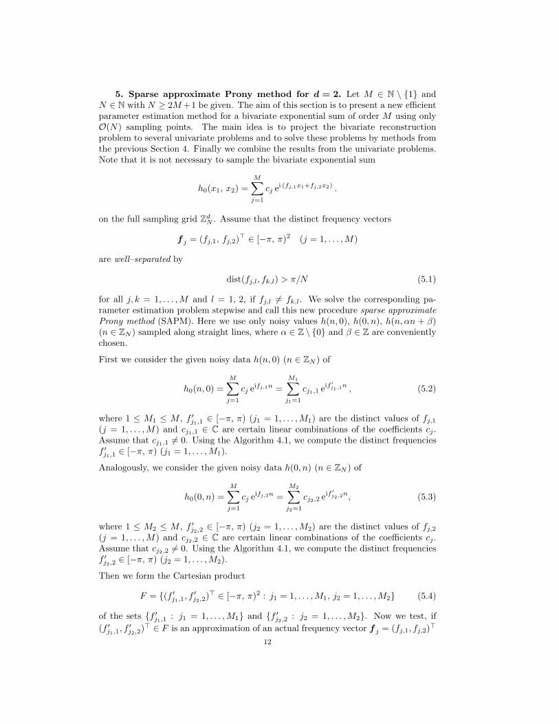
5. Sparse approximate Prony method for d = 2. Let M ∈ N \ {1} andN ∈ N with N ≥ 2M+1 be given. The aim of this section is to present a new efficientparameter estimation method for a bivariate exponential sum of order M using onlyO(N) sampling points. The main idea is to project the bivariate reconstructionproblem to several univariate problems and to solve these problems by methods fromthe previous Section 4. Finally we combine the results from the univariate problems.Note that it is not necessary to sample the bivariate exponential sum

h0(x1, x2) =

M∑j=1

cj ei (fj,1x1+fj,2x2) .

on the full sampling grid ZdN . Assume that the distinct frequency vectors

f j = (fj,1, fj,2)> ∈ [−π, π)2 (j = 1, . . . ,M)

are well–separated by

dist(fj,l, fk,l) > π/N (5.1)

for all j, k = 1, . . . ,M and l = 1, 2, if fj,l 6= fk,l. We solve the corresponding pa-rameter estimation problem stepwise and call this new procedure sparse approximateProny method (SAPM). Here we use only noisy values h(n, 0), h(0, n), h(n, αn + β)(n ∈ ZN ) sampled along straight lines, where α ∈ Z \ {0} and β ∈ Z are convenientlychosen.

First we consider the given noisy data h(n, 0) (n ∈ ZN ) of

h0(n, 0) =

M∑j=1

cj eifj,1n =

M1∑j1=1

cj1,1 eif′j1,1n , (5.2)

where 1 ≤ M1 ≤ M , f ′j1,1 ∈ [−π, π) (j1 = 1, . . . ,M1) are the distinct values of fj,1(j = 1, . . . ,M) and cj1,1 ∈ C are certain linear combinations of the coefficients cj .Assume that cj1,1 6= 0. Using the Algorithm 4.1, we compute the distinct frequenciesf ′j1,1 ∈ [−π, π) (j1 = 1, . . . ,M1).

Analogously, we consider the given noisy data h(0, n) (n ∈ ZN ) of

h0(0, n) =M∑j=1

cj eifj,2n =

M2∑j2=1

cj2,2 eif′j2,2n, (5.3)

where 1 ≤ M2 ≤ M , f ′j2,2 ∈ [−π, π) (j2 = 1, . . . ,M2) are the distinct values of fj,2(j = 1, . . . ,M) and cj2,2 ∈ C are certain linear combinations of the coefficients cj .Assume that cj2,2 6= 0. Using the Algorithm 4.1, we compute the distinct frequenciesf ′j2,2 ∈ [−π, π) (j2 = 1, . . . ,M2).

Then we form the Cartesian product

F = {(f ′j1,1, f′j2,2)> ∈ [−π, π)2 : j1 = 1, . . . ,M1, j2 = 1, . . . ,M2} (5.4)

of the sets {f ′j1,1 : j1 = 1, . . . ,M1} and {f ′j2,2 : j2 = 1, . . . ,M2}. Now we test, if

(f ′j1,1, f′j2,2

)> ∈ F is an approximation of an actual frequency vector f j = (fj,1, fj,2)>

12

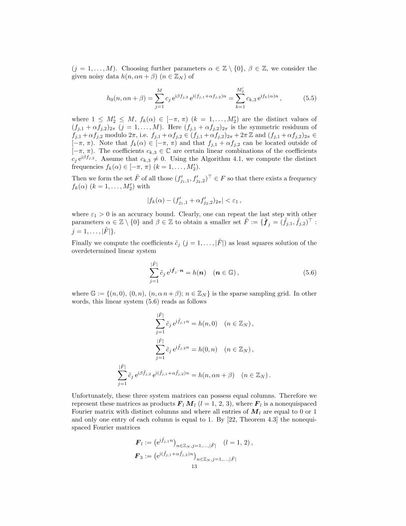
(j = 1, . . . ,M). Choosing further parameters α ∈ Z \ {0}, β ∈ Z, we consider thegiven noisy data h(n, αn+ β) (n ∈ ZN ) of

h0(n, αn+ β) =

M∑j=1

cj eiβfj,2 ei(fj,1+αfj,2)n =

M ′2∑k=1

ck,3 eifk(α)n , (5.5)

where 1 ≤ M ′2 ≤ M , fk(α) ∈ [−π, π) (k = 1, . . . ,M ′2) are the distinct values of(fj,1 + αfj,2)2π (j = 1, . . . ,M). Here (fj,1 + αfj,2)2π is the symmetric residuum offj,1 +αfj,2 modulo 2π, i.e. fj,1 +αfj,2 ∈ (fj,1 +αfj,2)2π + 2π Z and (fj,1 +αfj,2)2π ∈[−π, π). Note that fk(α) ∈ [−π, π) and that fj,1 + αfj,2 can be located outside of[−π, π). The coefficients ck,3 ∈ C are certain linear combinations of the coefficientscj eiβfj,2 . Assume that ck,3 6= 0. Using the Algorithm 4.1, we compute the distinctfrequencies fk(α) ∈ [−π, π) (k = 1, . . . ,M ′2).

Then we form the set F of all those (f ′j1,1, f′j2,2

)> ∈ F so that there exists a frequencyfk(α) (k = 1, . . . ,M ′2) with

|fk(α)− (f ′j1,1 + αf ′j2,2)2π| < ε1 ,

where ε1 > 0 is an accuracy bound. Clearly, one can repeat the last step with otherparameters α ∈ Z \ {0} and β ∈ Z to obtain a smaller set F := {f j = (fj,1, fj,2)> :

j = 1, . . . , |F |}.

Finally we compute the coefficients cj (j = 1, . . . , |F |) as least squares solution of theoverdetermined linear system

|F |∑j=1

cj eifj ·n = h(n) (n ∈ G) , (5.6)

where G := {(n, 0), (0, n), (n, αn+β); n ∈ ZN} is the sparse sampling grid. In otherwords, this linear system (5.6) reads as follows

|F |∑j=1

cj eifj,1n = h(n, 0) (n ∈ ZN ) ,

|F |∑j=1

cj eifj,2n = h(0, n) (n ∈ ZN ) ,

|F |∑j=1

cj eiβfj,2 ei(fj,1+αfj,2)n = h(n, αn+ β) (n ∈ ZN ) .

Unfortunately, these three system matrices can possess equal columns. Therefore werepresent these matrices as products F lM l (l = 1, 2, 3), where F l is a nonequispacedFourier matrix with distinct columns and where all entries of M l are equal to 0 or 1and only one entry of each column is equal to 1. By [22, Theorem 4.3] the nonequi-spaced Fourier matrices

F l :=(eifj,1n

)n∈ZN ,j=1,...,|F | (l = 1, 2) ,

F 3 :=(ei(fj,1+αfj,2)n

)n∈ZN ,j=1,...,|F |

13

possess left inverses Ll. If we introduce the vectors h1 := (h(n, 0))Nn=−N , h2 :=

(h(0, n))Nn=−N , h3 := (h(n, αn + β))Nn=−N , c := (cj)|F |j=1, and the diagonal matrix

D := diag (exp(iβfj,2))|F |j=1, we obtain the linear system

M1

M2

M3D

c =

L1 h1

L2 h2

L3 h3

. (5.7)

By a convenient choice of the parameters α ∈ Z \ {0} and β ∈ Z, the rank of theabove system matrix is equal to |F |. If this is not the case, we can use sampled valuesof h0 along another straight line. We summarize:

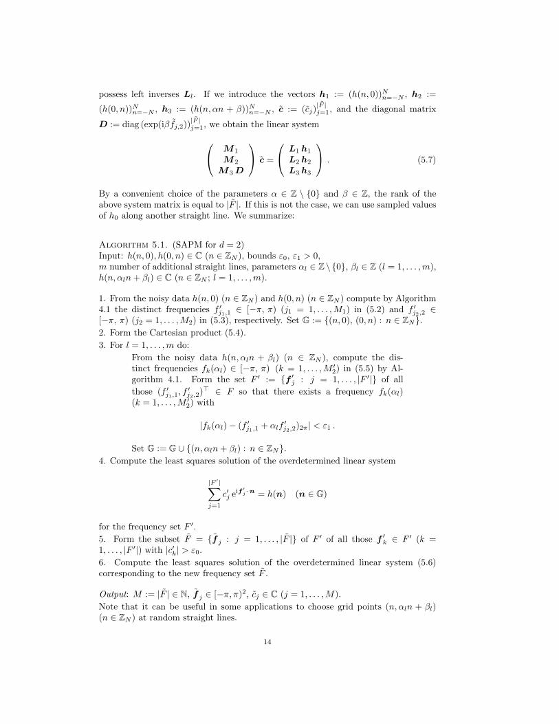
Algorithm 5.1. (SAPM for d = 2)Input: h(n, 0), h(0, n) ∈ C (n ∈ ZN ), bounds ε0, ε1 > 0,m number of additional straight lines, parameters αl ∈ Z \ {0}, βl ∈ Z (l = 1, . . . ,m),h(n, αln+ βl) ∈ C (n ∈ ZN ; l = 1, . . . ,m).

1. From the noisy data h(n, 0) (n ∈ ZN ) and h(0, n) (n ∈ ZN ) compute by Algorithm4.1 the distinct frequencies f ′j1,1 ∈ [−π, π) (j1 = 1, . . . ,M1) in (5.2) and f ′j2,2 ∈[−π, π) (j2 = 1, . . . ,M2) in (5.3), respectively. Set G := {(n, 0), (0, n) : n ∈ ZN}.2. Form the Cartesian product (5.4).

3. For l = 1, . . . ,m do:

From the noisy data h(n, αln + βl) (n ∈ ZN ), compute the dis-tinct frequencies fk(αl) ∈ [−π, π) (k = 1, . . . ,M ′2) in (5.5) by Al-gorithm 4.1. Form the set F ′ := {f ′j : j = 1, . . . , |F ′|} of all

those (f ′j1,1, f′j2,2

)> ∈ F so that there exists a frequency fk(αl)(k = 1, . . . ,M ′2) with

|fk(αl)− (f ′j1,1 + αlf′j2,2)2π| < ε1 .

Set G := G ∪ {(n, αln+ βl) : n ∈ ZN}.4. Compute the least squares solution of the overdetermined linear system

|F ′|∑j=1

c′j eif′j ·n = h(n) (n ∈ G)

for the frequency set F ′.

5. Form the subset F = {f j : j = 1, . . . , |F |} of F ′ of all those f ′k ∈ F ′ (k =1, . . . , |F ′|) with |c′k| > ε0.

6. Compute the least squares solution of the overdetermined linear system (5.6)corresponding to the new frequency set F .

Output: M := |F | ∈ N, f j ∈ [−π, π)2, cj ∈ C (j = 1, . . . ,M).

Note that it can be useful in some applications to choose grid points (n, αln + βl)(n ∈ ZN ) at random straight lines.

14

Remark 5.2. For the above parameter reconstruction, we have used sampled valuesof a bivariate exponentialsum h0 on m+ 2 straight lines. We have determined in thestep 3 of Algorithm 5.1 only a set F ′ which contains the set F of all exact frequencyvectors as a subset. This method is related to a result of A. Renyi [25] which isknown in discrete tomography: M distinct points in R2 are completely determined,if their orthogonal projections onto M + 1 arbitrary distinct straight lines throughthe origin are known. Let us additionally assume that ‖f j‖2 < π (j = 1, . . . ,M).Further let ϕ` ∈ [0, π) (` = 0, . . . ,M) be distinct angles. From sampled datah0(n cosϕ`, n sinϕ`) (n ∈ ZN ) we reconstruct the parameters fj,1 cosϕ`+fj,2 sinϕ`for j = 1, . . . ,M and ` = 0, . . . ,M . Since |fj,1 cosϕ` + fj,2 sinϕ`| < π, we have

(fj,1 cosϕ` + fj,2 sinϕ`)2π = fj,1 cosϕ` + fj,2 sinϕ` .

Thus fj,1 cosϕ`+fj,2 sinϕ` is equal to the distance between f j and the line x1 cosϕ`+x2 sinϕ` = 0, i.e., we know the orthogonal projection of f j onto the straight linex1 cosϕ` − x2 sinϕ` = 0. Hence we know that m ≤M − 1.

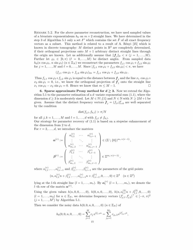
6. Sparse approximate Prony method for d ≥ 3. Now we extend the Algo-rithm 5.1 to the parameter estimation of a d–variate exponential sum (1.1), where thedimension d ≥ 3 is moderately sized. Let M ∈ N\{1} and N ∈ N with N ≥ 2M+1 begiven. Assume that the distinct frequency vectors f j = (fj,l)

dl=0 are well–separated

by the condition

dist(fj,l, fk,l) > π/N

for all j, k = 1, . . . ,M and l = 1, . . . , d with fj,l 6= fk,l.Our strategy for parameter recovery of (1.1) is based on a stepwise enhancement ofthe dimension from 2 to d.For r = 2, . . . , d, we introduce the matrices

α(r) :=

α(r)1,1 · · · α

(r)1,r−1

.... . .

...

α(r)mr,1

· · · α(r)mr,r−1

∈ (Z \ {0})mr×(r−1) ,

β(r) :=

β(r)1,1 · · · β

(r)1,r−1

.... . .

...

β(r)mr,1

· · · β(r)mr,r−1

∈ Zmr×(r−1) ,

where α(r)l,1 , . . . , α

(r)l,r−1 and β

(r)l,1 , . . . , β

(r)l,r−1 are the parameters of the grid points

(n, α(r)l,1n+ β

(r)l,1 , . . . , α

(r)l,r−1n+ β

(r)l,r−1, 0, . . . , 0) ∈ Zd (n ∈ Zd)

lying at the l-th straight line (l = 1, . . . ,mr). By α(r)l (l = 1, . . . ,mr), we denote the

l–th row of the matrix α(r).

Using the given values h(n, 0, 0, . . . , 0), h(0, n, 0, . . . , 0), h(n, α(2)l,1 n + β

(2)l,1 , 0, . . . , 0)

(l = 1, . . . ,m2) for n ∈ ZN , we determine frequency vectors (f ′j,1, f′j,2)> ∈ [−π, π)2

(j = 1, . . . ,M ′) by Algorithm 5.1.

Then we consider the noisy data h(0, 0, n, 0, . . . , 0) (n ∈ ZN ) of

h0(0, 0, n, 0, . . . , 0) =

M∑j=1

cj eifj,3n =

M3∑j3=1

cj3,3 eif′j3,3n,

15

where 1 ≤ M3 ≤ M , where f ′j3,3 ∈ [−π, π) (j3 = 1, . . . ,M3) the distinct valuesof fj,3 (j = 1, . . . ,M), and where cj3,3 ∈ C are certain linear combinations of thecoefficients cj . Assume that cj3,3 6= 0. Using the Algorithm 4.1, we compute thedistinct frequencies f ′j3,3 ∈ [−π, π) (j3 = 1, . . . ,M3). Now we form the Cartesianproduct

F := {(f ′j,1, f ′j,2, f ′j3,3)> ∈ [−π, π)3 : j = 1, . . . ,M ′; j3 = 1, . . . ,M3}

of the sets {(f ′j,1, f ′j,2)> : j = 1, . . . ,M ′} and {f ′j3,3 : j = 1, . . . ,M3}. Now we form asubset of F by using the data

h(n, α(3)l,1 n+ β

(3)l,1 , α

(3)l,2 n+ β

(3)l,2 , 0, . . . , 0) (l = 1, . . . ,m3) .

Since

h0(n, α(3)l,1 n+ β

(3)l,1 , α

(3)l,2 n+ β

(3)l,2 , 0, . . . , 0)

=

M∑j=1

cj ei(β(3)l,1 f

′j,2+β

(3)l,2 f

′j,3) ei(f

′j1,1+f

′j2,2α

(3)l,1+f

′j3,3α

(3)l,2 )n

=

M ′3∑k=1

ck,3 eifk(α(3)l )n ,

where 1 ≤ M ′3 ≤ M and where fk(α(3)l ) ∈ [−π, π) (k = 1, . . . ,M ′3) are the distinct

values of (f ′j,1 + α(3)l,1 f

′j,2 + α

(3)l,2 f

′j,3)2π. The coefficients ck,3 ∈ C are certain linear

combinations of the coefficients cj ei(β(3)l,1 f

′j,2+β

(3)l,2 f

′j,3). Then we form the set F ′ :=

{f ′j : j = 1, . . . , |F ′|} of all those (f ′j1,1, f′j2,2

, f ′j3,3)> ∈ F so that there exists a

frequency fk(α(3)l ) (k = 1, . . . ,M ′3) with

|fk(α(3)l )− (f ′j1,1 + f ′j2,2α

(3)l,1 + f ′j3,3α

(3)l,2 )2π| < ε1 .

Continuing analogously this procedure, we obtainAlgorithm 6.1. (SAPM for d ≥ 3)Input: h(n, 0, . . . , 0), h(0, n, 0, . . . , 0), . . . , h(0, . . . , 0, n) (n ∈ ZN ), bounds ε0, ε1 > 0,mr number of straight lines for dimension r = 2, . . . , d, parameters of straight linesα(r), β(r) ∈ Zmr×(r−1).

1. From the noisy data h(n, 0, . . . , 0), h(0, n, 0, . . . , 0), . . ., h(0, . . . , 0, n) (n ∈ ZN )compute by Algorithm 4.1 the distinct frequencies f ′jr,r ∈ [−π, π) (jr = 1, . . . ,Mr)for r = 1, . . . , d.Set G := {(n, 0, . . . , 0), . . . , (0, . . . , 0, n) : n ∈ ZN}.2. Set F := {f ′j1,1 : j1 = 1, . . . ,M1}.3. For r = 2, . . . , d do:

Form the Cartesian product

F := F×{f ′jr,r : jr = 1, . . . ,Mr} = {(f>l , f ′j,r)> : l = 1, . . . |F |, j = 1, . . . ,Mr} .

For l = 1, . . . ,mr do:For the noisy data

h(n, α(r)l,1n+β

(r)l,1 , . . . , α

(r)l,r−1n+β

(r)l,r−1, 0, . . . , 0) (n ∈ ZN ) ,

16

compute the distinct frequencies fk(α(r)l ) ∈ [−π, π) (k =

1, . . . ,M ′r) by Algorithm 4.1. Form the set F of all those(f ′j1,1, f

′j2,2

, . . . , f ′jr,r)> ∈ F so that there exists a frequency

fk(α(r)l ) with

|fk(α(r)l )− (f ′j1,1 + α

(r)l,1 fj2,2 + · · ·+ α

(r)l,r−1f

′jr,r)2π| < ε1 .

Set F := F and

G := G∪{(n, α(r)l,1n+β

(r)l,1 , . . . , α

(r)l,r−1n+β

(r)l,r−1, 0, . . . , 0) : n ∈ ZN}.

4. Compute the least squares solution of the overdetermined linear system

|F |∑j=1

c′j eifj ·n = h(n) (n ∈ G) (6.1)

for the frequency set F = {f j : j = 1, . . . , |F |}.5. Form the set F := {f j : j = 1, . . . , |F |} of all those fk ∈ F (k = 1, . . . , |F |) with|c′k| > ε0.6. Compute the least squares solution of the overdetermined linear system

|F |∑j=1

cj eifj ·n = h(n) (n ∈ G) (6.2)

corresponding to the new frequency set F = {f j : j = 1, . . . , |F |}.

Output: M := |F | ∈ N, f j ∈ [−π, π)d, cj ∈ C (j = 1, . . . ,M).

Remark 6.2. Note that we solve the overdetermined linear systems (6.1) and(6.2) only by using the values h(n) (n ∈ G), which we have used to determine thefrequencies f j . If more values h(n) are available, clearly one can use further values aswell in the final step to ensure a better least squares solvability of the linear systems,see (5.7) for the case d = 2 and Corollary 3.3. In addition we mention that there arevarious possibilities to combine the different dimensions, see e.g. Example 7.4.Remark 6.3. Our method can be interpreted as a reconstruction method for sparsemultivariate trigonometric polynomials from few samples, see [14, 12, 32] and the ref-erences therein. More precisely, let Πd

N denote the space of all d–variate trigonometricpolynomials of maximal order N . An element p ∈ Πd

N can be represented in the form

p(y) =∑k∈Zd

N

ck e2πik·y (y ∈ [−1

2,

1

2]d)

with ck ∈ C. There exist completely different methods for the reconstruction of“sparse trigonometric polynomials”, i.e., one assumes that the number M of thenonzero coefficients ck is much smaller than the dimension of Πd

N . Therefore ourmethod can be used with

h(x) := p(x

2N) =

M∑j=1

cj ei fj ·x (x ∈ [−N,N ]d),

17

and x = 2Ny and f j = πk/N if ck 6= 0. Using Algorithm 6.1, we find the frequencyvectors f j and the coefficients cj and we finally set k := round(Nf j/π), ck := cj . By[8] one knows sharp versions of L2–norm equivalences for trigonometric polynomialsunder the assumption that the sampling set contains no holes larger than the inversepolynomial degree, see also [2].

7. Numerical experiments. Finally, we apply the algorithms suggested in Sec-tion 5 to various examples. We have implemented our algorithms in MATLAB withIEEE double precision arithmetic. We compute the relative error of the frequenciesgiven by

e(f) := maxl=1,...,d

maxj=1,...,M

|fj,l − fj,l|

maxj=1,...,M

|fj,l|,

where fj,l are the frequency components computed by our algorithms. Analogously,the relative error of the coefficients is defined by

e(c) :=

maxj=1,...,M

|cj − cj |

maxj=1,...,M

|cj |,

where cj are the coefficients computed by our algorithms. Further we determine therelative error of the exponential sum by

e(h) :=max |h(x)− h(x)|

max |h(x)|,

where the maximum is built from approximately 10000 equispaced points from a gridof [−N,N ]d, and where

h(x) :=

M∑j=1

cj efj ·x

is the exponential sum recovered by our algorithms. We remark that the approxima-tion property of h and h in the uniform norm of the univariate method was shown in[21, Theorem 3.4]. We begin with an example previously considered in [28].Example 7.1. The bivariate exponential sum (1.1) taken from [28, Example 1]possesses the following parameters

(f>j )3j=1 =

0.48π 0.48π0.48π −0.48π−0.48π 0.48π

, (cj)3j=1 =

111

.

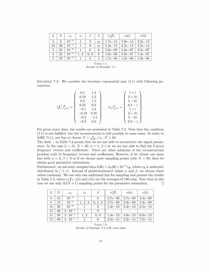
We sample this exponential sum (1.1) at the nodes h(k, 0), h(0, k) and h(k, αk + β),(k ∈ ZN ), where α, β ∈ Z are given in Table 7.1. Therefore the number of totalsampling points used in our method are only 3(2N + 1) or 4(2N + 1). Then weapply our Algorithm 5.1 for exact sampled data and for noisy sampled data h(k) =h(k) + 10−δ ek, where ek is uniformly distributed in [−1, 1]. The notation δ = ∞means that exact data are given. We present the chosen parameters and the resultsin Table 7.1. We choose same bounds ε0 = ε1 in Algorithm 5.1 and obtain very preciseresults even in the case, where the unknown number M = 3 is estimated by L.

18

L N ε0 α β δ e(f) e(c) e(h)

5 6 10−4 1 0 ∞ 1.7e−15 5.9e−14 3.2e−1310 20 10−4 1 0 ∞ 5.4e−15 4.5e−14 4.5e−145 25 10−3 1 0 6 5.6e−09 1.6e−07 2.5e−075 25 10−3 1, 2 0, 0 6 1.0e−08 5.9e−07 7.4e−075 25 10−3 1 0 5 1.7e−08 1.2e−06 1.3e−06

Table 7.1Results of Example 7.1.

Example 7.2. We consider the bivariate exponential sum (1.1) with following pa-rameters

(f>j )8j=1 =

0.1 1.20.19 1.30.3 1.50.35 0.3−0.1 1.2−0.19 0.35−0.3 −1.5−0.3 0.3

, (cj)

8j=1 =

1 + i2 + 3 i5− 6 i0.2− i1 + i

2 + 3 i5− 6 i0.2− i

.

For given exact data, the results are presented in Table 7.2. Note that the condition(5.1) is not fulfilled, but the reconstruction is still possible in some cases. In order tofulfill (5.1), one has to choose N > π

0.05 , i.e., N ≥ 63.

The dash − in Table 7.2 means that we are not able to reconstruct the signal param-eters. In the case L = 15, N = 30, α = 1, β = 0, we are not able to find the 8 givenfrequency vectors and coefficients. There are other solutions of the reconstructionproblem with 15 frequency vectors and coefficients. However, if we choose one moreline with α = 2, β = 0 or if we choose more sampling points with N = 80, then weobtain good parameter estimations.

Furthermore, we use noisy sampled data h(k) = h0(k)+10−δ ek, where ek is uniformlydistributed in [−1, 1]. Instead of predeterminated values α and β, we choose thesevalues randomly. We use only one additional line for sampling and present the resultsin Table 7.3, where e(f), e(c) and e(h) are the averages of 100 runs. Note that in thiscase we use only 3(2N + 1) sampling points for the parameter estimation.

L N ε0 α β e(f) e(c) e(h)

8 15 10−4 1 0 2.7e−09 5.7e−09 3.4e−098 15 10−4 1, 2, 3 0, 1, 2 2.7e−09 5.9e−09 3.3e−0915 30 10−4 1 0 1.4e−13 3.4e−13 6.5e−1315 30 2 · 10−1 1 0 – – –15 30 2 · 10−1 1, 2 0, 0 1.4e−13 4.0e−13 6.0e−1315 80 2 · 10−1 1 0 3.5e−15 3.2e−14 7.5e−14

Table 7.2Results of Example 7.2 with exact data.

19

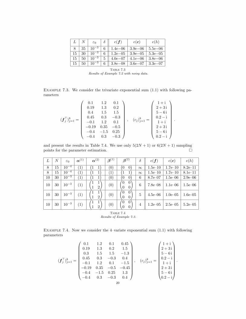
L N ε0 δ e(f) e(c) e(h)

8 35 10−3 6 1.4e−06 3.9e−06 5.5e−0615 30 10−3 6 1.2e−05 3.9e−05 5.3e−0515 50 10−3 5 4.0e−07 4.1e−06 3.8e−0615 50 10−3 6 3.8e−08 3.6e−07 3.3e−07

Table 7.3Results of Example 7.2 with noisy data.

Example 7.3. We consider the trivariate exponential sum (1.1) with following pa-rameters

(f>j )8j=1 =

0.1 1.2 0.10.19 1.3 0.20.4 1.5 1.50.45 0.3 −0.3−0.1 1.2 0.1−0.19 0.35 −0.5−0.4 −1.5 0.25−0.4 0.3 −0.3

, (cj)

8j=1 =

1 + i2 + 3 i5− 6 i0.2− i1 + i

2 + 3 i5− 6 i0.2− i

.

and present the results in Table 7.4. We use only 5(2N + 1) or 6(2N + 1) samplingpoints for the parameter estimation.

L N ε0 α(1) α(2) β(1) β(2) δ e(f) e(c) e(h)

8 15 10−4 (1)(1 1

)(0)

(0 0

)∞ 1.5e–10 1.7e–10 8.2e–11

8 15 10−4 (1)(1 1

)(1)

(1 1

)∞ 1.5e–10 1.7e–10 8.1e–11

10 30 10−3 (1)(1 1

)(0)

(0 0

)6 8.7e–07 1.5e–06 2.9e–06

10 30 10−3 (1)

(1 11 2

)(0)

(0 00 0

)6 7.8e–08 1.1e–06 1.5e–06

10 30 10−3 (1)

(1 11 2

)(0)

(0 00 0

)5 4.5e–06 1.0e–05 1.6e–05

10 30 10−3 (1)

(1 11 2

)(0)

(0 00 0

)4 1.2e–05 2.5e–05 5.2e–05

Table 7.4Results of Example 7.3.

Example 7.4. Now we consider the 4–variate exponential sum (1.1) with followingparameters

(f>j )8j=1 =

0.1 1.2 0.1 0.450.19 1.3 0.2 1.50.3 1.5 1.5 −1.30.45 0.3 −0.3 0.4−0.1 1.2 0.1 −1.5−0.19 0.35 −0.5 −0.45−0.4 −1.5 0.25 1.3−0.4 0.3 −0.3 0.4

, (cj)

8j=1 =

1 + i2 + 3 i5− 6 i0.2− i1 + i

2 + 3 i5− 6 i0.2− i

.

20

Instead of using Algorithm 6.1 directly, we apply the Algorithm 5.1 for the first twovariables and then for the last variables with the parameters α(2) and β(2). Then wetake the tensor product of the obtained two parameter sets and use the additionalparameters from α(4) and β(4) in order to find a reduced set. Finally we solve theoverdetermined linear system. The results are presented in Table 7.5. We use only7(2N + 1) or 10(2N + 1) sampling points for the parameter estimation.

L N ε0 α(2) α(4) β(2) β(4) δ e(f) e(c) e(h)

8 15 10−4 1(1 1 1

)0

(0 0 0

)∞ 1.7e-10 2.5e-11 1.6e-10

8 15 10−4 1(1 1 1

)1

(1 1 1

)∞ 1.7e-10 2.4e-11 1.6e-10

15 30 10−4 1(1 1 1

)0

(0 0 0

)∞ 1.3e-14 6.4e-15 8.8e-14

15 30 10−3 1(1 1 1

)0

(0 0 0

)6 1.0e-06 3.2e-07 3.0e-06

15 30 10−3 1(1 1 1

)0

(0 0 0

)5 1.3e-05 3.4e-06 4.2e-05

15 30 10−3

(1−1

) (1 1 1−1 1 −1

) (00

) (0 0 00 0 0

)6 1.1e-06 2.7e-07 3.9e-06

15 30 10−3

(1−1

) (1 1 1−1 1 −1

) (00

) (0 0 00 0 0

)5 8.8e-06 1.9e-06 3.3e-05

15 50 10−3

(1−1

) (1 1 1−1 1 −1

) (00

) (0 0 00 0 0

)5 4.5e-07 1.2e-07 1.6e-06

15 50 10−3

(1−1

) (1 1 1−1 1 −1

) (00

) (0 0 00 0 0

)4 8.0e-07 2.4e-07 1.1e-05

Table 7.5Results of Example 7.4.

Acknowledgment. The authors thank Franziska Nestler for the numerical ex-periments. The first named author gratefully acknowledges the support by the Ger-man Research Foundation within the project PO 711/10–1. Furthermore, the authorswould like to thank the reviewers for their helpful comments to improve this paper.

REFERENCES

[1] F. Andersson, M. Carlsson, and M.V. de Hoop. Nonlinear approximation of functions in twodimensions by sums of exponential functions. Appl. Comput. Harmon. Anal. 29:156 – 181,2010.

[2] R. F. Bass and K. Grochenig. Random sampling of multivariate trigonometric polynomials.SIAM J. Math. Anal. 36:773 – 795, 2004.

[3] G. Beylkin and L. Monzon. On approximations of functions by exponential sums. Appl. Comput.Harmon. Anal. 19:17 – 48, 2005.

[4] D. Braess. Nonlinear Approximation Theory. Springer, Berlin, 1986.[5] O. Christensen. An Introduction to Frames and Riesz Bases. Birkhauser, Boston, 2003.[6] P.L. Dragotti, M. Vetterli, and T. Blu. Sampling moments and reconstructing signals of finite

rate of innovation: Shannon meets Strang–Fix. IEEE Trans. Signal Process. 55:1741 – 1757,2007.

[7] G.H. Golub and C.F. Van Loan. Matrix Computations. 3rd ed. Johns Hopkins Univ. Press,Baltimore, 1996.

[8] K. Grochenig. Reconstruction algorithms in irregular sampling. Math. Comput. 59:181 – 194,1992.

[9] N.J. Higham. Functions of Matrices: Theory and Computation. SIAM, Philadelphia, 2008.[10] Y. Hua and T.K. Sarkar. Matrix pencil method for estimating parameters of exponentially

damped/undamped sinusoids in noise. IEEE Trans. Acoust. Speech Signal Process. 38:814– 824, 1990.

[11] A.E. Ingham. Some trigonometrical inequalities with applications to the theory of series. Math.Z. 41:367 – 379, 1936.

[12] M.A. Iwen. Combinatorial sublinear–time Fourier algorithms. Found. Comput. Math., 10:303–338, 2010.

[13] J. Keiner, S. Kunis, and D. Potts. Using NFFT3 - a software library for various nonequispacedfast Fourier transforms. ACM Trans. Math. Software 36:Article 19, 1 – 30, 2009.

21

[14] S. Kunis and H. Rauhut. Random sampling of sparse trigonometric polynomials II, Orthogonalmatching pursuit versus basis pursuit. Found. Comput. Math. 8:737 – 763, 2008.

[15] V. Komornik and P. Loreti. Fourier Series in Control Theory. Springer, New York, 2005.[16] V. Komornik and P. Loreti. Semi–discrete Ingham–type inequalities. Appl. Math. Optim. 55:203

– 218, 2007.[17] A.M. Lindner. A universal constant for exponential Riesz sequences. Z. Anal. Anw. 19:553 –

559, 2000.[18] J. M. Papy, L. De Lathauwer, and S. Van Huffel. Exponential data fitting using multilinear

algebra: the decimative case. J. Chemometrics 23:341 – 351, 2004.[19] V. Pereyra and G. Scherer. Exponential data fitting. In V. Pereyra and G. Scherer, editors.

Exponential Data Fitting and its Applications, pp. 1 – 26. Bentham Science Publ., Sharjah,2010.

[20] V. Pereyra and G. Scherer. Exponential Data Fitting and its Applications. Bentham SciencePubl., Sharjah, 2010.

[21] T. Peter, D. Potts, and M. Tasche. Nonlinear approximation by sums of exponentials andtranslates. SIAM J. Sci. Comput. 33:1920 – 1947, 2011.

[22] D. Potts and M. Tasche. Numerical stability of nonequispaced fast Fourier transforms. J.Comput. Appl. Math. 222:655 – 674, 2008.

[23] D. Potts and M. Tasche. Parameter estimation for exponential sums by approximate Pronymethod. Signal Process. 90:1631 – 1642, 2010.

[24] D. Potts and M. Tasche. Parameter estimation for nonincreasing exponential sums by Prony–likemethods. Preprint, Chemnitz University of Technology, 2012.

[25] A. Renyi. On projections of probability distributions. Acta Math. Acad. Sci. Hung., 3:131 –142, 1952.

[26] R. Roy and T. Kailath. ESPRIT – estimation of signal parameters via rotational invariancetechniques. IEEE Trans. Acoustic Speech Signal Process. 37:984 – 994, 1989.

[27] R. Roy and T. Kailath. ESPRIT – estimation of signal parameters via rotational invariancetechniques. In L. Auslander, F.A. Grunbaum, J.W. Helton, T. Kailath, P. Khargoneka, S.Mitter, editors. Signal Processing, Part II: Control Theory and Applications, pp. 369 – 411.Springer, New York, 1990.

[28] J.J. Sacchini, W.M. Steedy and R.L. Moses. Two–dimensional Prony modeling parameterestimation. IEEE Trans. Signal Process. 41:3127 – 3137, 1993.

[29] T.K. Sarkar and O. Pereira. Using the matrix pencil method to estimate the parameters of asum of complex exponentials. IEEE Antennas and Propagation Magazine 37:48 – 55, 1995.

[30] P. Shukla and P.L. Dragotti. Sampling schemes for multidimensional signals with finite rate ofinnovation. IEEE Trans. Signal Process. 55:3670 – 3686, 2007.

[31] M. Vetterli, P. Marziliano, and T. Blu. Sampling signals with finite rate of innovation. IEEETrans. Signal Process. 50:1417 – 1428, 2002.

[32] Z. Xu. Deterministic sampling of sparse trigonometric polynomials. J. Complexity 27:133 – 140,2011.

22