Embed Size (px)
Citation preview

1
Peter Fox
Data Analytics – ITWS-4963/ITWS-6965
Week 10a, April 1, 2014
Support Vector Machines
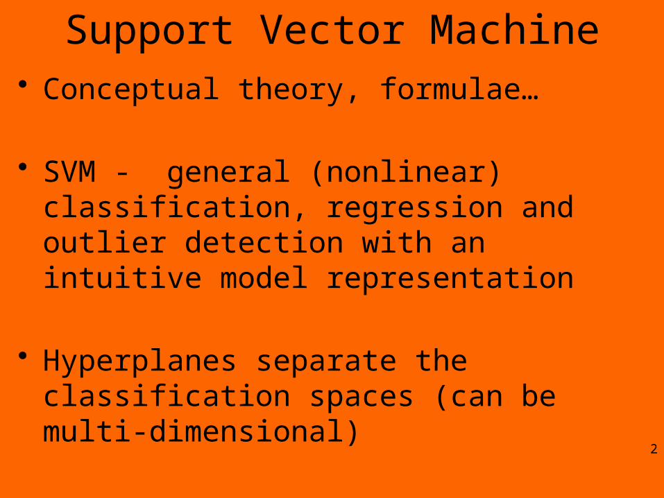
Support Vector Machine• Conceptual theory, formulae…
• SVM - general (nonlinear) classification, regression and outlier detection with an intuitive model representation
• Hyperplanes separate the classification spaces (can be multi-dimensional)
• Kernel functions can play a key role 2
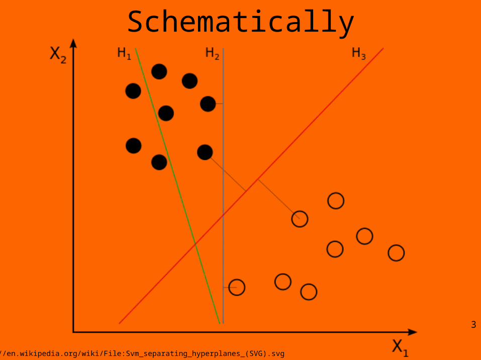
Schematically
3
http://en.wikipedia.org/wiki/File:Svm_separating_hyperplanes_(SVG).svg
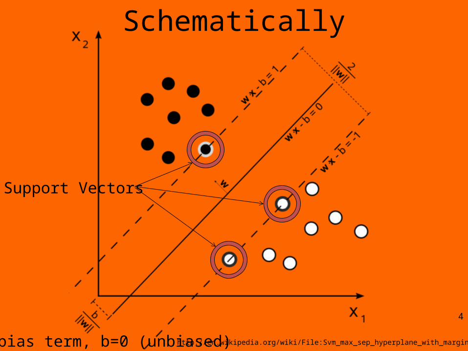
Schematically
4
http://en.wikipedia.org/wiki/File:Svm_max_sep_hyperplane_with_margin.pngb=bias term, b=0 (unbiased)
Support Vectors
Construction• Construct an optimization objective function
that is inherently subject to some constraints– Like minimizing least square error (quadratic)
• Most important: the classifier gets the points right by “at least” the margin
• Support Vectors can then be defined as those points in the dataset that have "non zero” Lagrange multipliers*. – make a classification on a new point by using
only the support vectors – why?5
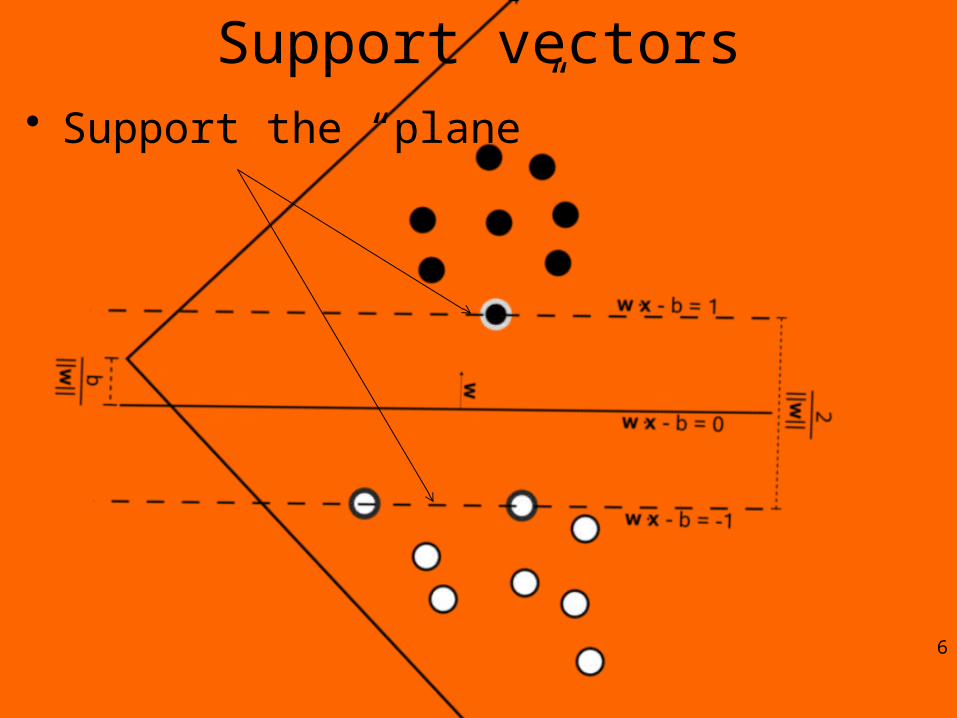
Support vectors• Support the “plane”
6
What about the “machine” part• Ignore it – somewhat leftover from the
“machine learning” era– It is trained and then– Classifies
7
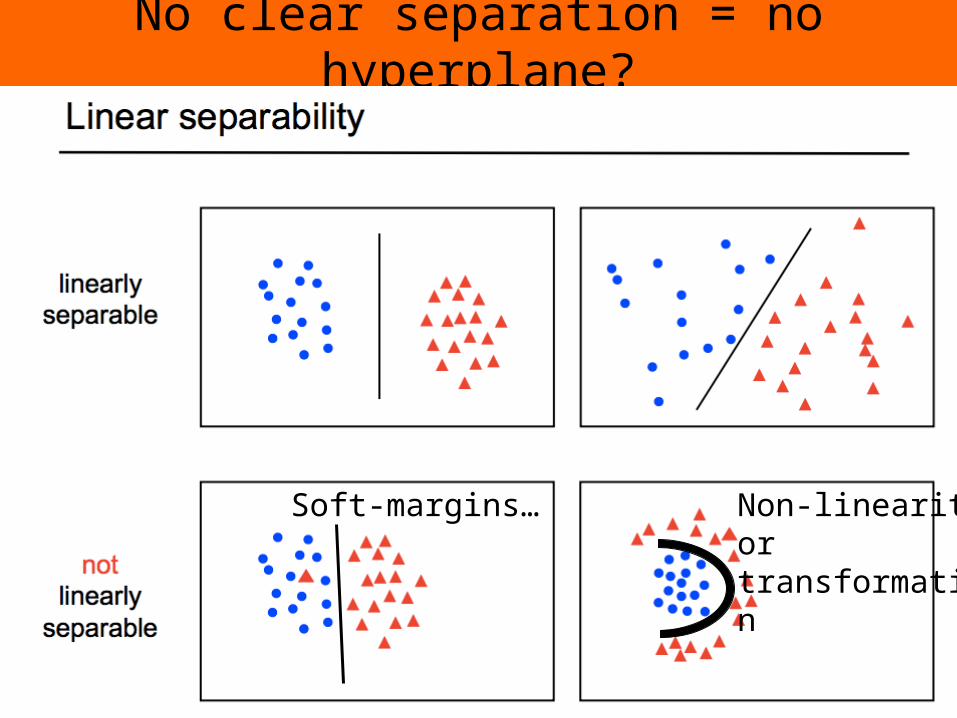
No clear separation = no hyperplane?
8
Soft-margins… Non-linearity or transformation
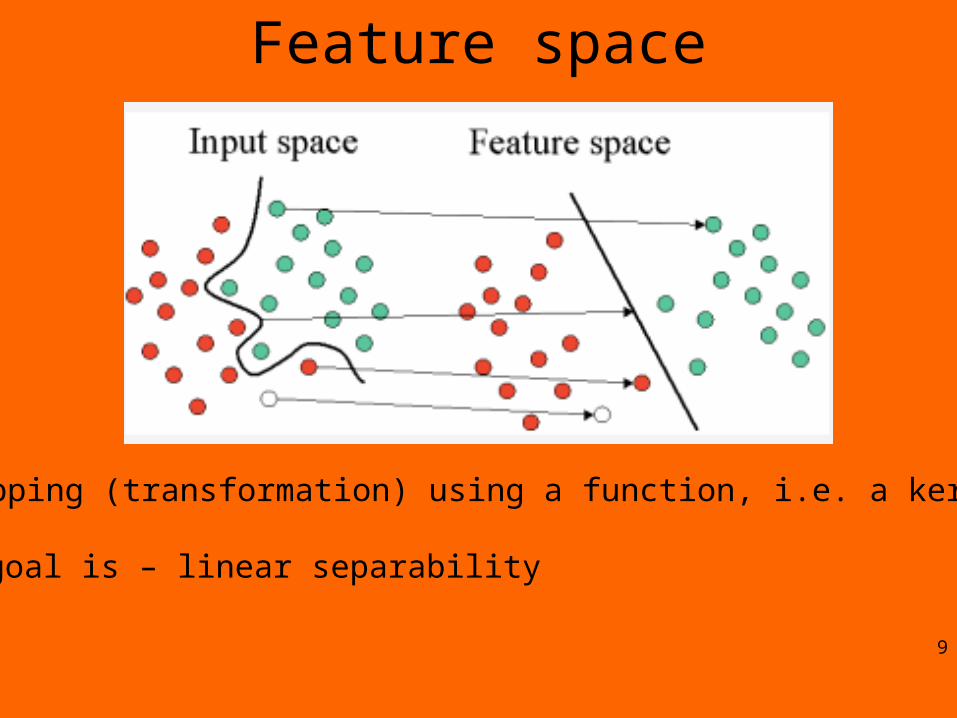
Feature space
9
Mapping (transformation) using a function, i.e. a kernel
goal is – linear separability

Kernels or “non-linearity”…
10
the kernel function, represents a dot product of input data points mapped into the higher dimensional feature space by transformation phi + note presence of “gamma” parameter
http://www.statsoft.com/Textbook/Support-Vector-Machines
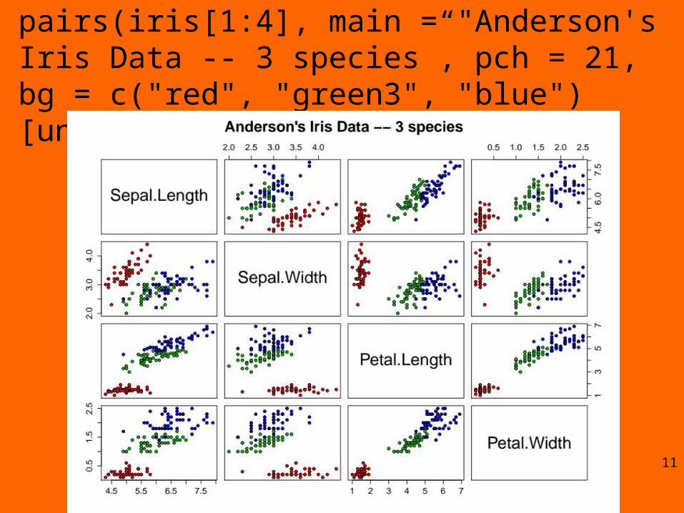
pairs(iris[1:4], main = "Anderson's Iris Data -- 3 species”, pch = 21, bg = c("red", "green3", "blue")[unclass(iris$Species)])
11
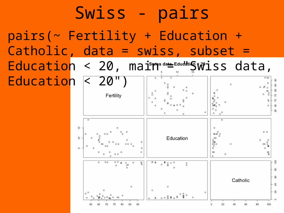
Swiss - pairs
12
pairs(~ Fertility + Education + Catholic, data = swiss, subset = Education < 20, main = "Swiss data, Education < 20")
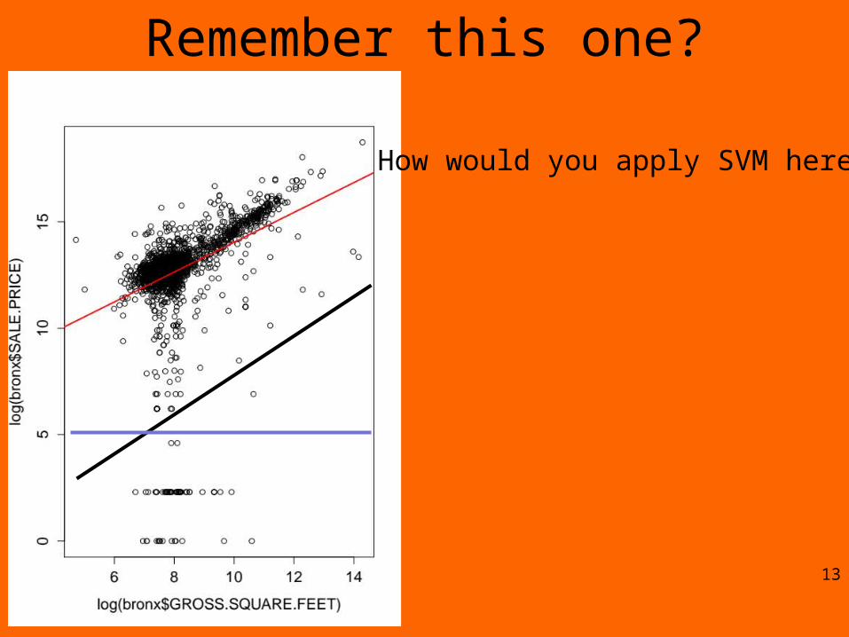
Remember this one?
13
How would you apply SVM here?
Outlier detection• SVMs have also been extended to deal with
the problem of novelty detection (or one-class classification)
• Detection works by creating a spherical decision boundary around a set of data points by a set of support vectors describing the sphere’s boundary
14
Multiple classification• In addition to these heuristics for extending a
binary SVM to the multi-class problem, there have been reformulations of the support vector quadratic problem that deal with more than two classes
• One of the many approaches for native support vector multi-class classification works by solving a single optimization problem including the data from all classes (spoc-svc)
15
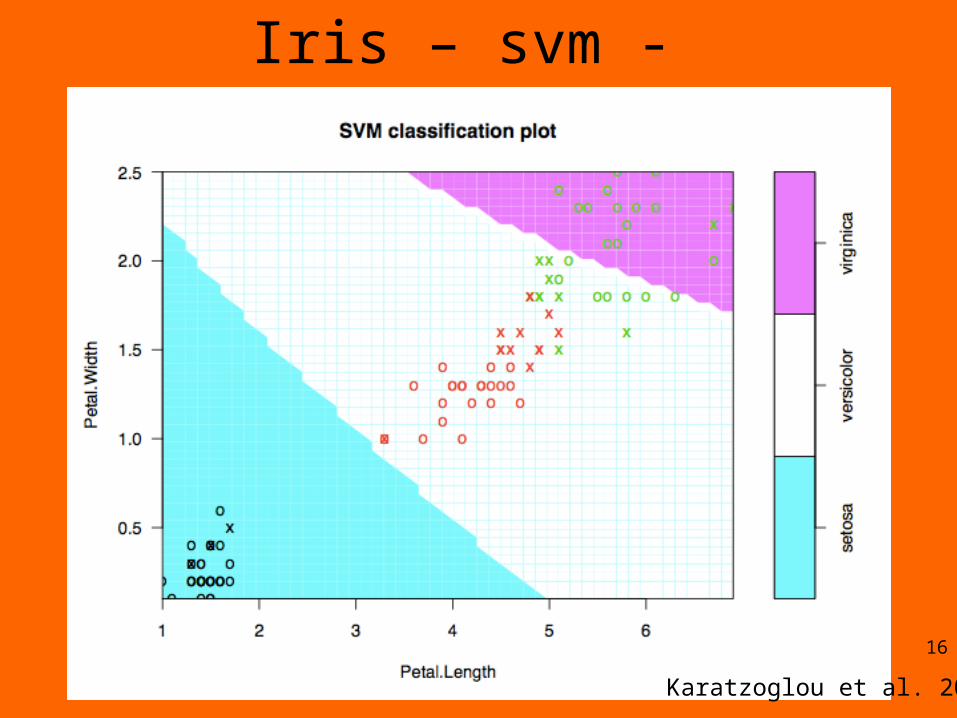
Iris – svm -
16
Karatzoglou et al. 2006

17
Karatzoglou et al. 2006
kernlab, svmpath and klaR• http://escience.rpi.edu/data/DA/v15i09.pdf
• Work through the examples – how did these go?– Familiar datasets and samples procedures from 4
libraries (these are the most used)– kernlab– e1071– svmpath– klaR
18
Karatzoglou et al. 2006
Application of SVM• Classification, outlier, regression…• Can produce labels or probabilities (and
when used with tree partitioning can produce decision values)
• Different minimizations functions subject to different constraints (Lagrange multipliers)
• Observe the effect of changing the C parameter and the kernel
19
See Karatzoglou et al. 2006

Types of SVM (names)• Classification SVM Type 1 (also known as C-
SVM classification)• Classification SVM Type 2 (also known as nu-
SVM classification)• Regression SVM Type 1 (also known as
epsilon-SVM regression)• Regression SVM Type 2 (also known as nu-
SVM regression)
20

More kernels
21
Karatzoglou et al. 2006
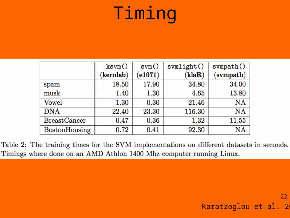
Timing
22
Karatzoglou et al. 2006
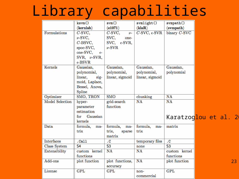
Library capabilities
23
Karatzoglou et al. 2006
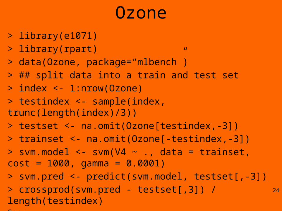
Ozone> library(e1071)
> library(rpart)
> data(Ozone, package=“mlbench”)
> ## split data into a train and test set
> index <- 1:nrow(Ozone)
> testindex <- sample(index, trunc(length(index)/3))
> testset <- na.omit(Ozone[testindex,-3])
> trainset <- na.omit(Ozone[-testindex,-3])
> svm.model <- svm(V4 ~ ., data = trainset, cost = 1000, gamma = 0.0001)
> svm.pred <- predict(svm.model, testset[,-3])
> crossprod(svm.pred - testset[,3]) / length(testindex)See: http://cran.r-project.org/web/packages/e1071/vignettes/svmdoc.pdf 24
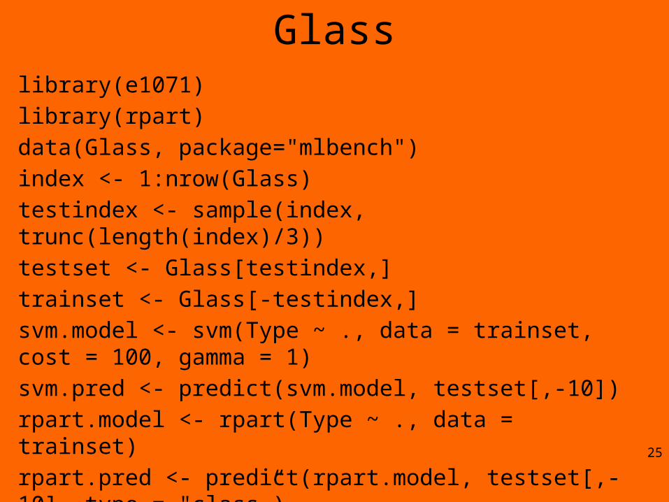
Glasslibrary(e1071)
library(rpart)
data(Glass, package="mlbench")
index <- 1:nrow(Glass)
testindex <- sample(index, trunc(length(index)/3))
testset <- Glass[testindex,]
trainset <- Glass[-testindex,]
svm.model <- svm(Type ~ ., data = trainset, cost = 100, gamma = 1)
svm.pred <- predict(svm.model, testset[,-10])
rpart.model <- rpart(Type ~ ., data = trainset)
rpart.pred <- predict(rpart.model, testset[,-10], type = "class”)25
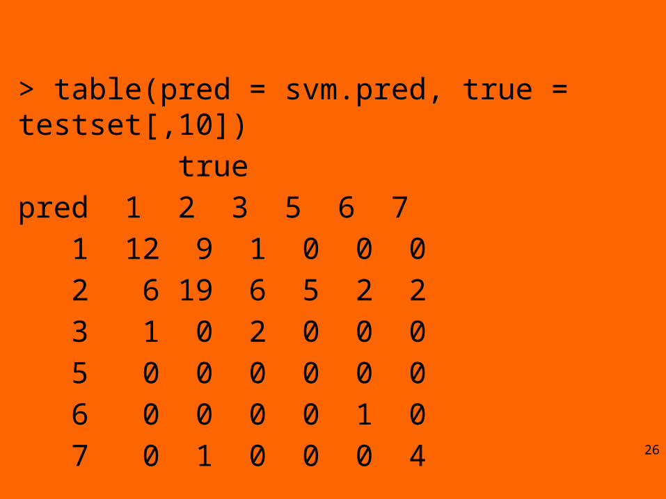
> table(pred = svm.pred, true = testset[,10])
true
pred 1 2 3 5 6 7
1 12 9 1 0 0 0
2 6 19 6 5 2 2
3 1 0 2 0 0 0
5 0 0 0 0 0 0
6 0 0 0 0 1 0
7 0 1 0 0 0 426
kernlab• http://escience.rpi.edu/data/DA/svmbasic_not
es.pdf
• Some scripts: Lab9b_<n>_2014.R
27
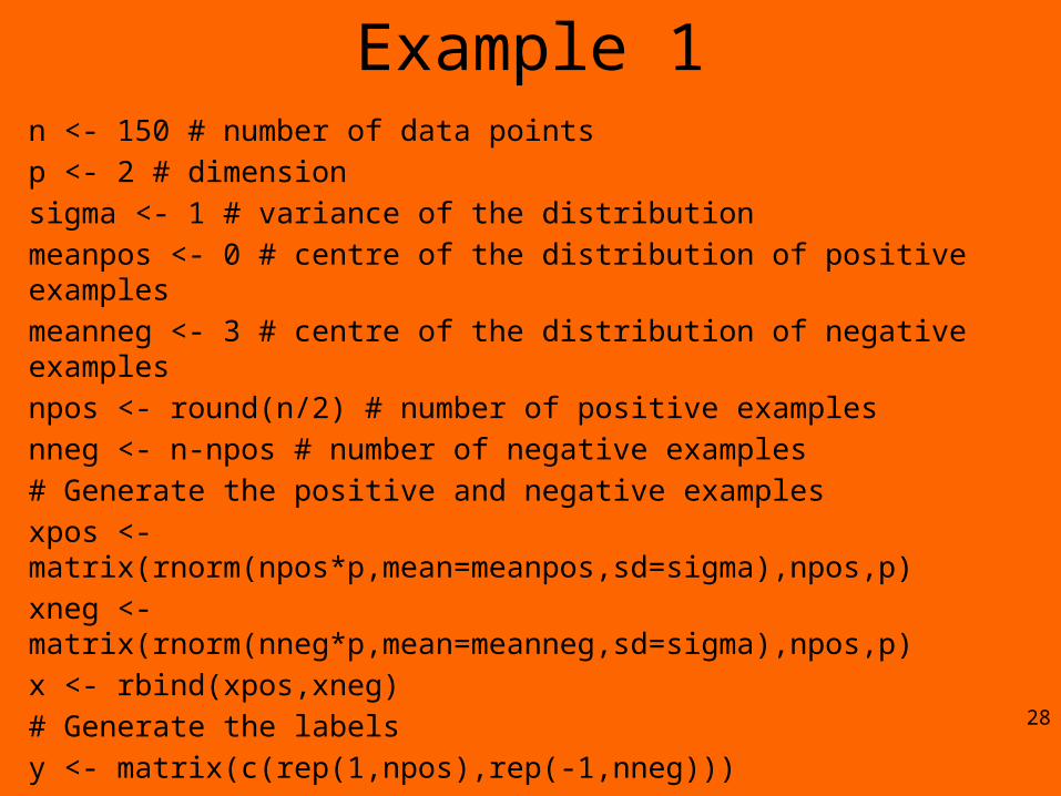
Example 1n <- 150 # number of data points
p <- 2 # dimension
sigma <- 1 # variance of the distribution
meanpos <- 0 # centre of the distribution of positive examples
meanneg <- 3 # centre of the distribution of negative examples
npos <- round(n/2) # number of positive examples
nneg <- n-npos # number of negative examples
# Generate the positive and negative examples
xpos <- matrix(rnorm(npos*p,mean=meanpos,sd=sigma),npos,p)
xneg <- matrix(rnorm(nneg*p,mean=meanneg,sd=sigma),npos,p)
x <- rbind(xpos,xneg)
# Generate the labels
y <- matrix(c(rep(1,npos),rep(-1,nneg)))
# Visualize the data
plot(x,col=ifelse(y>0,1,2))
legend("topleft",c('Positive','Negative'),col=seq(2),pch=1,text.col=seq(2))28
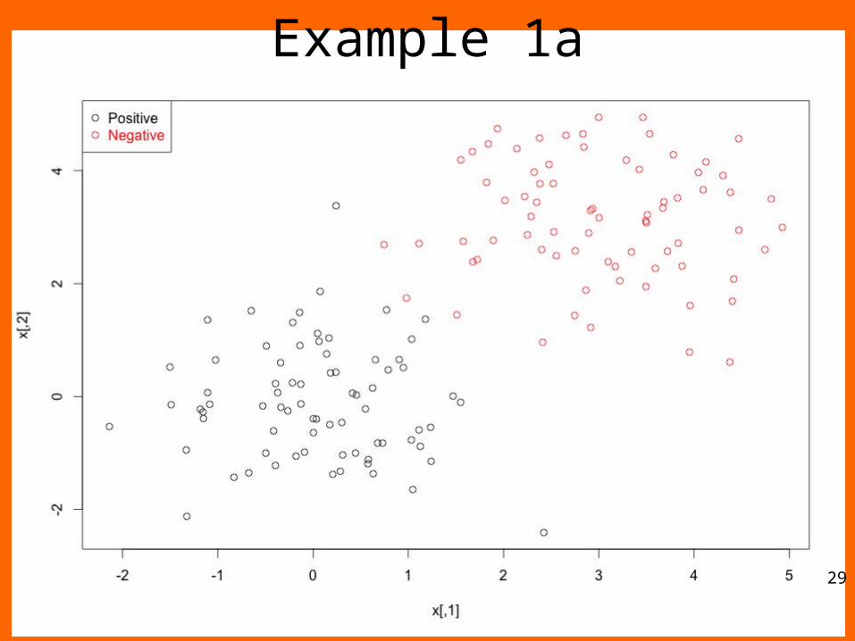
Example 1a
29
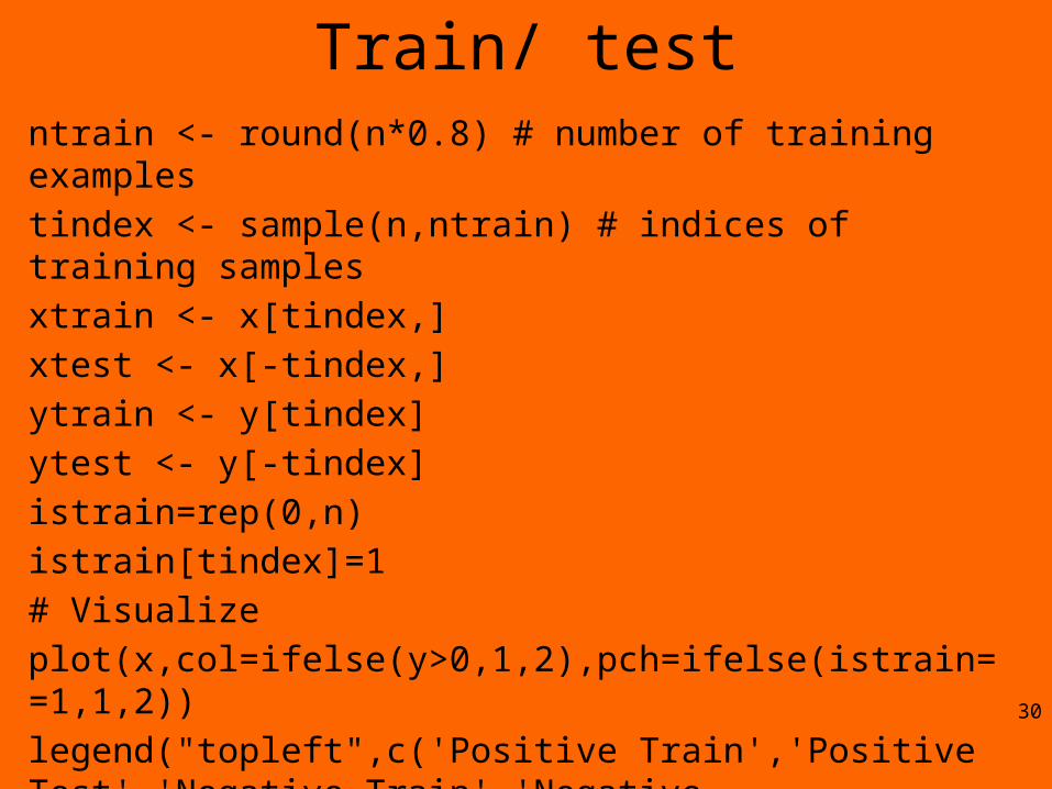
Train/ testntrain <- round(n*0.8) # number of training examples
tindex <- sample(n,ntrain) # indices of training samples
xtrain <- x[tindex,]
xtest <- x[-tindex,]
ytrain <- y[tindex]
ytest <- y[-tindex]
istrain=rep(0,n)
istrain[tindex]=1
# Visualize
plot(x,col=ifelse(y>0,1,2),pch=ifelse(istrain==1,1,2))
legend("topleft",c('Positive Train','Positive Test','Negative Train','Negative Test'),col=c(1,1,2,2), pch=c(1,2,1,2), text.col=c(1,1,2,2)) 30
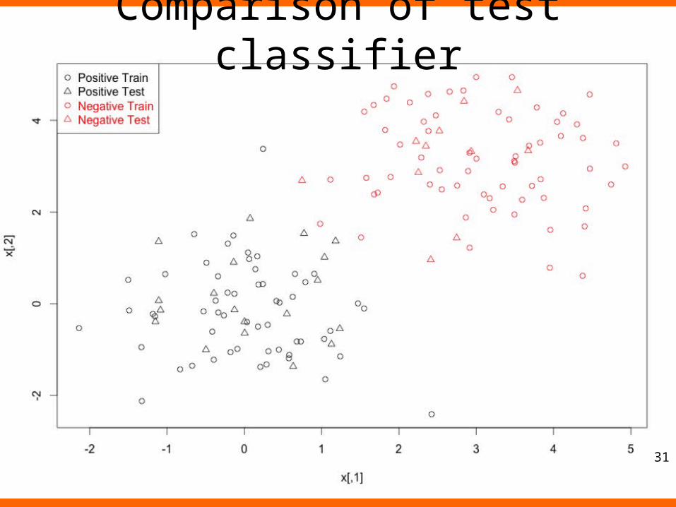
Comparison of test classifier
31
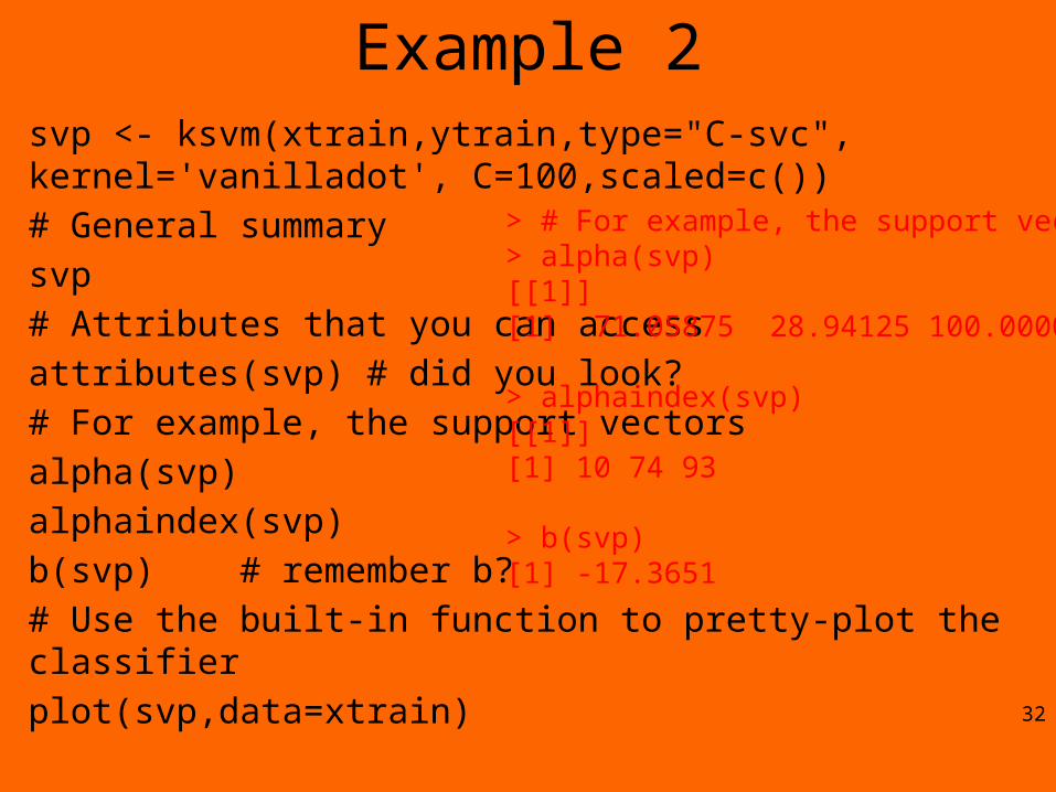
Example 2svp <- ksvm(xtrain,ytrain,type="C-svc", kernel='vanilladot', C=100,scaled=c())
# General summary
svp
# Attributes that you can access
attributes(svp) # did you look?
# For example, the support vectors
alpha(svp)
alphaindex(svp)
b(svp) # remember b?
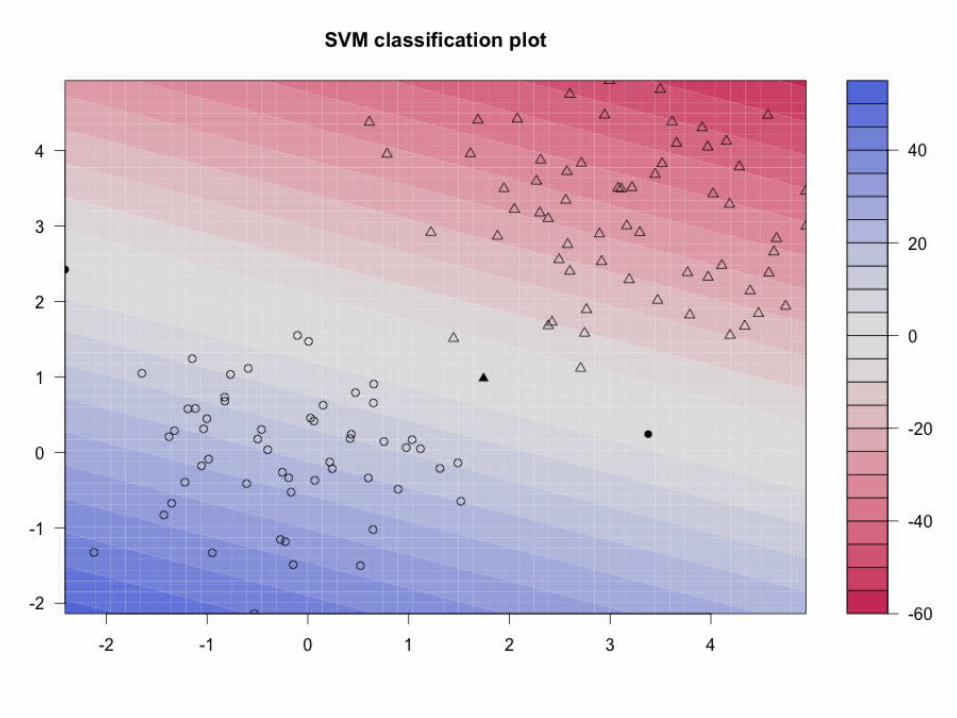
# Use the built-in function to pretty-plot the classifier
plot(svp,data=xtrain)32
> # For example, the support vectors> alpha(svp)[[1]][1] 71.05875 28.94125 100.00000
> alphaindex(svp)[[1]][1] 10 74 93
> b(svp)[1] -17.3651
33

ALL dataset (was dropped)• http://www.stjuderesearch.org/site/data/ALL1/
34
R-SVM• http://www.stanford.edu/group/wonglab/RSV
Mpage/r-svm.tar.gz
• http://www.stanford.edu/group/wonglab/RSVMpage/R-SVM.html – Read/ skim the paper– Explore this method on a dataset of your choice,
e.g. one of the R built-in datasets
35

Reading some papers…• They provide a guide to the type of project
report you may prepare…
36

Assignment to come…
• Assignment 7: Predictive and Prescriptive Analytics. Due ~ week ~11. 20%..
37

Admin info (keep/ print this slide)• Class: ITWS-4963/ITWS 6965• Hours: 12:00pm-1:50pm Tuesday/ Friday• Location: SAGE 3101• Instructor: Peter Fox• Instructor contact: [email protected], 518.276.4862 (do not
leave a msg)• Contact hours: Monday** 3:00-4:00pm (or by email appt)• Contact location: Winslow 2120 (sometimes Lally 207A
announced by email)• TA: Lakshmi Chenicheri [email protected] • Web site: http://tw.rpi.edu/web/courses/DataAnalytics/2014
– Schedule, lectures, syllabus, reading, assignments, etc.
38