1 Pertemuan 08 Pengujian Hipotesis Matakuliah: A0392 – Statistik Ekonomi Tahun: 2006

1

Pertemuan 08Pengujian Hipotesis

Matakuliah : A0392 – Statistik Ekonomi

Tahun : 2006

2

Outline Materi :

• Uji hipotesis rata-rata

• Uji hipotesis beda rata-rata peubah bebas

• Uji hipotesis beda rata-rata peubah berpasangan

3

Inference from Small Samples

I

Some graphic screen captures from Seeing Statistics ®Some images © 2001-(current year) www.arttoday.com

4

Introduction

• When the sample size is small, the estimation and testing procedures of large samples are not appropriate.

• There are equivalent small sample test and estimation procedures for , the mean of a normal populationthe difference between two population

means2, the variance of a normal populationThe ratio of two population variances.

5

The Sampling Distribution of the Sample Mean

• When we take a sample from a normal population, the sample mean has a normal distribution for any sample size n, and

• has a standard normal distribution. • But if is unknown, and we must use s to estimate it,

the resulting statistic is not normalis not normal.

n

xz

/

n

xz

/

normal!not is / ns

x normal!not is / ns

x

x

6

Student’s t Distribution

• Fortunately, this statistic does have a sampling distribution that is well known to statisticians, called the Student’s t distribution, Student’s t distribution, with nn-1 -1 degrees of freedom.degrees of freedom.

ns

xt

/

ns

xt

/

•We can use this distribution to create estimation testing procedures for the population mean .

7

Properties of Student’s t

• Shape depends on the sample size n or the degrees of degrees of freedom, freedom, nn-1.-1.

• As n increase , variability of t decrease because the estimate s is based on more and more information.

• As n increases the shapes of the t and z distributions become almost identical.

•Mound-shapedMound-shaped and symmetric about 0.

•More variable than More variable than zz, with “heavier tails”

AppletApplet

8

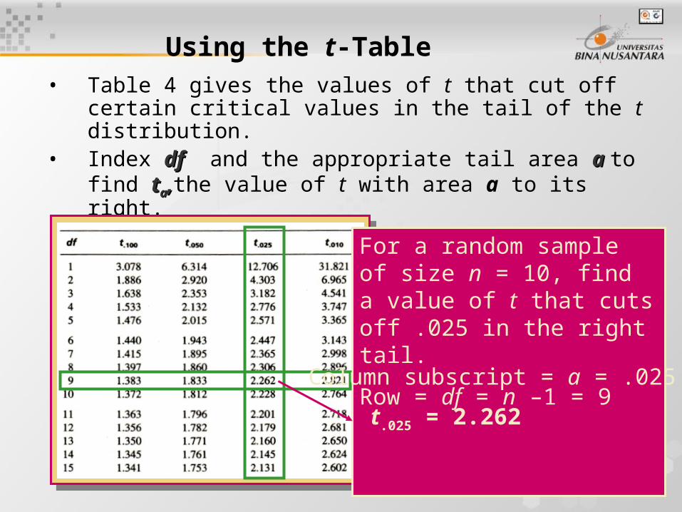
Using the t-Table

• Table 4 gives the values of t that cut off certain critical values in the tail of the t distribution.

• Index dfdf and the appropriate tail area a a to find ttaa,,the value of t with area a to its right.

For a random sample of size n = 10, find a value of t that cuts off .025 in the right tail.

Row = df = n –1 = 9

t.025 = 2.262

Column subscript = a = .025

9

Small Sample Inference for a Population Mean

• The basic procedures are the same as those used for large samples. For a test of hypothesis:

.1on with distributi- ta

on basedregion rejection aor values- using/

statistic test theusing

tailedor two one :H versus:HTest

0

a00

ndf

pns

xt


on basedregion rejection aor values- using/


tailedor two one :H versus:HTest

0

a00

ndf

pns

xt

10

• For a 100(1)% confidence interval for the population mean

.1on with distributi- ta of tailin the

/2 area off cuts that of value theis where 2/

2/

ndf

ttn

stx

.1on with distributi- ta of tailin the

/2 area off cuts that of value theis where 2/

2/

ndf

ttn

stx

Small Sample Inference for a Population Mean

11

Example

A sprinkler system is designed so that the average time for the sprinklers to activate after being turned on is no more than 15 seconds. A test of 5 systems gave the following times:

17, 31, 12, 17, 13, 25 Is the system working as specified? Test using = .05.

specified) as ng(not worki 15:H

specified) as (working 15:H

a

0

specified) as ng(not worki 15:H

specified) as (working 15:H

a

0

12

Example

Data:Data: 17, 31, 12, 17, 13, 25First, calculate the sample mean and standard deviation, using your calculator or the formulas in Chapter 2.

387.75

6115

2477

1

)(

167.196

115

222

nnx

xs

n

xx i

387.75

6115

2477

1

)(

167.196

115

222

nnx

xs

n

xx i

13

ExampleData:Data: 17, 31, 12, 17, 13, 25Calculate the test statistic and find the rejection region for =.05.

5161 38.16/387.7

15167.19

/

:freedom of Degrees :statisticTest

0

ndfns

xt

5161 38.16/387.7

15167.19

/

:freedom of Degrees :statisticTest

0

ndfns

xt

Rejection Region: Reject H0 if t > 2.015. If the test statistic falls in the rejection region, its p-value will be less than = .05.

Rejection Region: Reject H0 if t > 2.015. If the test statistic falls in the rejection region, its p-value will be less than = .05.

14

Conclusion

Data:Data: 17, 31, 12, 17, 13, 25Compare the observed test statistic to the rejection region, and draw conclusions.

.015.2 if HReject

:RegionRejection

38.1 :statisticTest

0

t

t

.015.2 if HReject

:RegionRejection

38.1 :statisticTest

0

t

t

Conclusion: For our example, t = 1.38 does not fall in the rejection region and H0 is not rejected. There is insufficient evidence to indicate that the average activation time is greater than 15.

15:H

15:H

a

0

15:H

15:H

a

0

15

Approximating the p-value

• You can only approximate the p-value for the test using Table 4.

Since the observed value of t = 1.38 is smaller than t.10 = 1.476,

p-value > .10.

16

The exact p-value

• You can get the exact p-value using some calculators or a computer.

One-Sample T: TimesTest of mu = 15 vs mu > 15

Variable N Mean StDev SE MeanTimes 6 19.17 7.39 3.02

Variable 95.0% Lower Bound T PTimes 13.09 1.38 0.113

One-Sample T: TimesTest of mu = 15 vs mu > 15

Variable N Mean StDev SE MeanTimes 6 19.17 7.39 3.02

Variable 95.0% Lower Bound T PTimes 13.09 1.38 0.113

p-value = .113 which is greater than .10 as we approximated using Table 4.

AppletApplet

17

Testing the Difference between Two Means

normal. be must spopulation two the small, are sizes sample the Since

and variancesand and means with2 and 1 spopulation from

drawn are and size of samples random tindependen 9,Chapter in As22

21 .21

21

μμ

nn

normal. be must spopulation two the small, are sizes sample the Since

and variancesand and means with2 and 1 spopulation from

drawn are and size of samples random tindependen 9,Chapter in As22

21 .21

21

μμ

nn

•To test: •H0:D0 versus Ha:one of three

where D0 is some hypothesized difference, usually 0.

18


•The test statistic used in Chapter 9

•does not have either a z or a t distribution, and cannot be used for small-sample inference. •We need to make one more assumption, that the population variances, although unknown, are equal.

2

22

1

21

21z

ns

ns

xx

2

22

1

21

21z

ns

ns

xx

19


•Instead of estimating each population variance separately, we estimate the common variance with

2

)1()1(

21

222

2112

nn

snsns

2

)1()1(

21

222

2112

nn

snsns

21

2

021

11

nns

Dxxt

21

2

021

11

nns

Dxxt

has a t distribution with n1+n2-2=(n1-1)+(n2-1) degrees of freedom.

•And the resulting test statistic,

20

Estimating the Difference between Two Means

•You can also create a 100(1-)% confidence interval for 1-2.

2

)1()1( with

21

222

2112

nn

snsns

2

)1()1( with

21

222

2112

nn

snsns

21

22/21

11)(

nnstxx

21

22/21

11)(

nnstxx

Remember the three assumptions:

1. Original populations normal

2. Samples random and independent

3. Equal population variances.

Remember the three assumptions:

1. Original populations normal

2. Samples random and independent

3. Equal population variances.

21

Example• Two training procedures are compared by

measuring the time that it takes trainees to assemble a device. A different group of trainees are taught using each method. Is there a difference in the two methods? Use = .01.

Time to Assemble

Method 1 Method 2

Sample size 10 12

Sample mean 35 31

Sample Std Dev

4.9 4.5

0:H 210

21

2

21

11

0

:statisticTest

nns

xxt

0:H 21a

22

Example

• Solve this problem by approximating the p-value using Table 4.

Time to Assemble

Method 1 Method 2

Sample size 10 12

Sample mean 35 31

Sample Std Dev 4.9 4.5

99.1

121

101

942.21

3135

:statisticTest

t

AppletApplet

942.2120

)5.4(11)9.4(9

2

)1()1(

:Calculate

22

21

222

2112

nn

snsns

23

Example

value)-(2

1)99.1(

)99.1()99.1( :value-

ptP

tPtPp

value)-(2

1)99.1(

)99.1()99.1( :value-

ptP

tPtPp

.025 < ½( p-value) < .05

.05 < p-value < .10

Since the p-value is greater than = .01, H0 is not rejected. There is insufficient evidence to indicate a difference in the population means.

.025 < ½( p-value) < .05

.05 < p-value < .10

Since the p-value is greater than = .01, H0 is not rejected. There is insufficient evidence to indicate a difference in the population means.

df = n1 + n2 – 2 = 10 + 12 – 2 = 20df = n1 + n2 – 2 = 10 + 12 – 2 = 20

24


•How can you tell if the equal variance assumption is reasonable?

statistic. test ealternativan use

,3smaller

larger ratio, theIf

.reasonable is assumption varianceequal the

,3smaller

larger ratio, theIf

:Thumb of Rule

2

2

2

2

s

s

s

s

statistic. test ealternativan use

,3smaller

larger ratio, theIf

.reasonable is assumption varianceequal the

,3smaller

larger ratio, theIf

:Thumb of Rule

2

2

2

2

s

s

s

s

25


•If the population variances cannot be assumed equal, the test statistic

•has an approximate t distribution with degrees of freedom given above. This is most easily done by computer.

2

22

1

21

21

ns

ns

xxt

2

22

1

21

21

ns

ns

xxt

1)/(

1)/(

2

22

22

1

21

21

2

2

22

1

21

nns

nns

ns

ns

df

1)/(

1)/(

2

22

22

1

21

21

2

2

22

1

21

nns

nns

ns

ns

df

26

The Paired-Difference Test

•Sometimes the assumption of independent samples is intentionally violated, resulting in a matched-pairsmatched-pairs or paired-difference testpaired-difference test.•By designing the experiment in this way, we can eliminate unwanted variability in the experiment by analyzing only the differences,

ddii = = xx11ii – – xx22ii

•to see if there is a difference in the two population means,

27

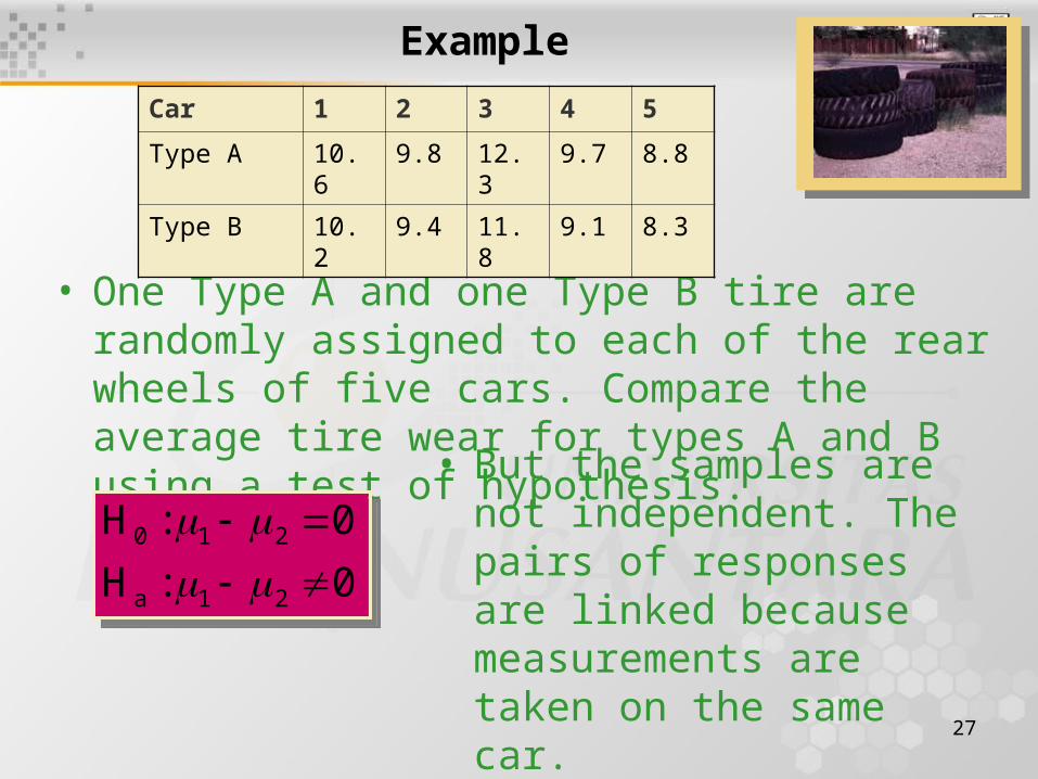
Example

• One Type A and one Type B tire are randomly assigned to each of the rear wheels of five cars. Compare the average tire wear for types A and B using a test of hypothesis.

Car 1 2 3 4 5

Type A 10.6 9.8 12.3 9.7 8.8

Type B 10.2 9.4 11.8 9.1 8.3

0:H

0:H

21a

210

0:H

0:H

21a

210

• But the samples are not independent. The pairs of responses are linked because measurements are taken on the same car.

28

The Paired-Difference Test


on basedregion rejection aor value- theUse

. s,difference theofdeviation standard andmean

theare and pairs, ofnumber where

/

0


0 :H test we0:H test To d0210

ndf

p

d

sdn

ns

dt

i

d

d


on basedregion rejection aor value- theUse

. s,difference theofdeviation standard andmean

theare and pairs, ofnumber where

/

0


0 :H test we0:H test To d0210

ndf

p

d

sdn

ns

dt

i

d

d

29

Example

Car 1 2 3 4 5

Type A 10.6 9.8 12.3 9.7 8.8

Type B 10.2 9.4 11.8 9.1 8.3

Difference .4 .4 .5 .6 .5

0:H

0:H

21a

210

0:H

0:H

21a

210

.0837

.48 Calculate

1

22

nn

dd

s

n

dd

ii

d

i

.0837

.48 Calculate

1

22

nn

dd

s

n

dd

ii

d

i 8.125/0837.

048.

/

0

:statisticTest

ns

dt

d

8.125/0837.

048.

/

0

:statisticTest

ns

dt

d

30

Example

CarCar 1 2 3 4 5

Type A 10.6 9.8 12.3 9.7 8.8

Type B 10.2 9.4 11.8 9.1 8.3

Difference .4 .4 .5 .6 .5

Rejection region: Reject H0 if t > 2.776 or t < -2.776.

Conclusion: Since t = 12.8, H0 is rejected. There is a difference in the average tire wear for the two types of tires.

31

Some Notes

•You can construct a 100(1-)% confidence interval for a paired experiment using

•Once you have designed the experiment by pairing, you MUST analyze it as a paired experiment. If the experiment is not designed as a paired experiment in advance, do not use this procedure.

n

std d

2/n

std d

2/

32

Key Concepts

I. Experimental Designs for Small SamplesI. Experimental Designs for Small Samples

1. Single random sample: The sampled population must be normal.

2. Two independent random samples: Both sampled populations must be normal.

a. Populations have a common variance 2.

b. Populations have different variances

3. Paired-difference or matched-pairs design: The samples are not independent.

33

Key Concepts

Documents

1 Pertemuan 08 Pengujian Hipotesis Matakuliah: A0392 – Statistik Ekonomi Tahun: 2006