Embed Size (px)
Citation preview

1
Performance evaluation of object detectionalgorithms for video surveillance
Jacinto Nascimento⋆, Member, IEEE Jorge [email protected] [email protected]
IST/ISR, Torre Norte, Av. Rovisco Pais, 1049-001, Lisboa Portugal
EDICS: 4-SEGMAbstract
In this paper we propose novel methods to evaluate the performance of object detection algorithms in videosequences. This procedure allows us to highlight characteristics (e.g., region splitting or merging) which are specificof the method being used. The proposed framework compares the output of the algorithm with the ground truthand measures the differences according to objective metrics. In this way it is possible to perform a fair comparisonamong different methods, evaluating their strengths and weaknesses and allowing the user to perform a reliablechoice of the best method for a specific application. We applythis methodology to segmentation algorithms recentlyproposed and describe their performance. These methods were evaluated in order to assess how well they can detectmoving regions in an outdoor scene in fixed-camera situations.
Index Terms
Surveillance Systems, Performance Evaluation, Metrics, Ground Truth, Segmentation, Multiple Interpretations.
I. I NTRODUCTION
V IDEO surveillance systems rely on the ability to detect moving objects in the video stream which is a relevant
information extraction step in a wide range of computer vision applications. Each image is segmented by
automatic image analysis techniques. This should be done in areliable and effective way in order to cope with
unconstrained environments, non stationary background and different object motion patterns. Furthermore, different
types of objects are manually considered e.g., persons, vehicles or groups of people.
Many algorithms have been proposed for object detection in video surveillance applications. They rely on different
assumptions e.g., statistical models of the background [1]–[3], minimization of Gaussian differences [4], minimum
and maximum values [5], adaptivity [6,7] or a combination offrame differences and statistical background models
[8]. However, few information is available on the performance of these algorithms for different operating conditions.
Two approaches have been recently considered to characterize the performance of video segmentation algorithms:
pixel-based methods, template based methods and object-based methods. Pixel based methods assume that we wish
to detect all the active pixels in a given image. Object detection is therefore formulated as a set of independent
pixel detection problems. This is a classic binary detectionproblem provided that we know the ground truth (ideal
segmented image). The algorithms can therefore be evaluatedby standard measures used in Communication theory
e.g., misdetection rate, false alarm rate and receiver operating characteristic (ROC) [9].
This work was supported by FCT under the project LTT and by EU project CAVIAR (IST-2001-37540).Corresponding Author: Jacinto Nascimento, (email:[email protected]), Complete Address: Instituto Superior Tecnico-Instituto
de Sistemas e Robotica (IST/ISR), Av. Rovisco Pais, Torre Norte, 6o piso, 1049-001, Lisboa, PORTUGALPhone: +351-21-8418270,Fax:+351-21-8418291

2
Several proposals have been made to improve the computation of the ROC in video segmentation problems e.g.,
using a perturbation detection rate analysis [10] or an equilibrium analysis [11]. The usefulness of pixel-based
methods for surveillance applications is questionable since we are not interested in the detection of point targets
but object regions instead. The computation of the ROC can also be performed using rectangular regions selected
by the user, with and without moving objects [12]. This improves the evaluation strategy since the statistics are
based on templates instead of isolated pixels.
A third class of methods is based on an object evaluation. Most of the works aim to characterize color, shape and
path fidelity by proposing figures of merit for each of these issues [13]–[15] or area based performance evaluation
as in [16]. This approach is instrumental to measure the performance of image segmentation methods for video
coding and synthesis but it is not usually used in surveillance applications.
These approaches have three major drawbacks. First object detection is not a classic binary detection problem.
Several types of errors should be considered (not just misdetection and false alarms). For examplewhat should we
do if a moving object is split into several active regions ? or if two objects are merged into a single region ? Second
some methods are based on the selection of isolated pixels orrectangular regions with and without persons. This
is an unrealistic assumption since practical algorithms have to segment the image into background and foreground
and do not have to classify rectangular regions selected by the user. Third, it is not possible to define a unique
ground truth. Many images admit several valid segmentations. If the image analysis algorithm produces a valid
segmentation its output should be considered as correct.
In this paper we propose objective metrics to evaluate the performance of object detection methods by comparing
the output of the video detector with the ground truth obtained by manual edition. Several types of errors are
considered: splits of foreground regions; merges of foreground regions; simultaneous split and merge of foreground
regions; false alarms, and detection failures. False alarms occur when false objects are detected. The detection
failures are caused by missing regions which have not been detected.
In this paper five segmentation algorithms are considered asexamples and evaluated. We also consider multiple
interpretations in the case of ambiguous situations e.g., when it is not clear if two objects overlap and should be
considered as a group or if they are separated apart.
The first algorithm is denoted as basic background subtraction(BBS) algorithm. It computes the absolute
difference between the current image and a static background image and compares each pixel to a threshold.
All the connected components are computed and they are considered as active regions if their area exceeds a
given threshold. This is perhaps the simplest object detection algorithm one can imagine. The second method is the
detection algorithm used in theW4 system [17]. Three features are used to characterize each pixel of the background
image: minimum intensity, maximum intensity and maximum absolute difference in consecutive frames. The third
method assumes that each pixel of the background is a realization of a random variable with Gaussian distribution
(SGM - Single Gaussian Model) [1]. The mean and covariance of the Gaussian distribution are independently
estimated for each pixel. The fourth algorithm represents the distribution of the background pixels with a mixture
of Gaussians [2]. Some modes correspond to the background andsome are associated with active regions (MGM
- Multiple Gaussian Model). The last method is the one proposed in [18] and denoted asLehigh Omnidirectional

3
Tracking System (LOTS). It is tailored to detect small non cooperative targets such as snipers. Some of these
algorithms are described in a special issue of IEEE transactions on PAMI (August 2001), which describes a state
of art methods for automatic surveillance systems.
In this work we provide segmentation results of these algorithms on the PETS2001 sequences, using the proposed
framework. The main features of the proposed method are the following. Given the correct segmentation of the
video sequence we detect several types of errorsi) splits of foreground regions,ii) merges of foreground regions,
iii) simultaneously split and merge of foreground regions,iv) false alarms (detection of false objects) andv) the
detection failures (missing active regions). We then compute statistics for each type of error.
The structure of the paper is as follows. Section 2 briefly reviews previous work. Section 3 describes the
segmentation algorithms used in this paper. Section 4 describes the proposed framework. Experimental tests are
discussed in Section 5 and Section 6 presents the conclusions.
II. RELATED WORK
Surveillance and monitoring systems often require on line segmentation of all moving objects in a video
sequence. Segmentation is a key step since it influences the performance of the other modules, e.g., object tracking,
classification or recognition. For instance, if object classification is required, an accurate detection is needed to
obtain a correct classification of the object.
Background subtraction is a simple approach to detect moving objects in video sequences. The basic idea is
to subtract the current frame from a background image and to classify each pixel as foreground or background
by comparing the difference with a threshold [19]. Morphological operations followed by a connected component
analysis are used to compute all active regions in the image.In practice, several difficulties arise: the background
image is corrupted by noise due to camera movements and fluttering objects (e.g., trees waving), illumination
changes, clouds, shadows. To deal with these difficulties several methods have been proposed (see [20]).
Some works use a deterministic background model e.g., by characterizing the admissible interval for each pixel
of the background image as well as the maximum rate of change in consecutive images or the median of largest
inter-frames absolute difference [5,17]. Most works however rely on statistical models of the background, assuming
that each pixel is a random variable with a probability distribution estimated from the video stream. For example, the
Pfinder system (“Person Finder”) uses a Gaussian model to describe each pixel of the background image [1]. A more
general approach consists of using a mixture of Gaussians torepresent each pixel. This allows the representation
of multi modal distributions which occur in natural scene (e.g., in the case of fluttering trees) [2].
Another set of algorithms is based on spatio-temporal segmentation of the video signal. These methods try to
detect moving regions taking into account not only the temporal evolution of the pixel intensities and color but also
their spatial properties. Segmentation is performed in a 3D region of image-time space, considering the temporal
evolution of neighbor pixels. This can be done in several wayse.g., by using spatio-temporal entropy, combined
with morphological operations [21]. This approach leads to an improvement of the systems performance, compared
with traditional frame difference methods. Other approaches are based on the 3D structure tensor defined from
the pixels spatial and temporal derivatives, in a given timeinterval [22]. In this case, detection is based on the
Mahalanobis distance, assuming a Gaussian distribution for the derivatives. This approach has been implemented
4
in real time and tested with PETS 2005 data set. Other alternatives have also been considered e.g., the use of a
region growing method in 3D space-time [23].
A significant research effort has been done to cope with shadows and with nonstationary backgrounds. Two
types of changes have to be considered: show changes (e.g., due to the sun motion) and rapid changes (e.g., due to
clouds, rain or abrupt changes in static objects). Adaptivemodels and thresholds have been used to deal with slow
background changes [18]. These techniques recursively update the background parameters and thresholds in order to
track the evolution of the parameters in nonstationary operating conditions. To cope with abrupt changes, multiple
model techniques have been proposed [18] as well as predictive stochastic models (e.g., AR, ARMA [24,25]).
Another difficulty is the presence of ghosts [26], i.e., falseactive regions due to statics objects belonging to
the background image (e.g., cars) which suddenly start to move. This problem has been addressed by combining
background subtraction with frame differencing or by high level operations [27],[28].
III. SEGMENTATION ALGORITHMS
This section describes object detection algorithms used in this work:BBS, W4, SGM , MGM andLOTS. The
BBS, SGM , MGM algorithms use color whileW4 andLOTS use gray scale images. In theBBS algorithm,
the moving objects are detected by computing the differencebetween the current frame and the background image.
A thresholding operation is performed to classify each pixel as foreground region if
|It(x, y)− µt(x, y)| > T, (1)
where It(x, y) is a 3 × 1 vector being the intensity of the pixel in the current frame and µt(x, y) is the mean
intensity (background) of the pixel,T is a constant.
Ideally, pixels associated with the same object should havethe same label. This can be accomplished by
performing a connected component analysis (e.g., using 8 - connectivity criterion). This step is usually performed
after a morphological filtering (dilation and erosion) to eliminate isolated pixels and small regions.
The second algorithm is denoted here asW4 since it is used in theW4 system to compute moving objects
[17]. This algorithm is designed for grayscale images. The background model is built using a training sequence
without persons or vehicles. Three values are estimated for each pixel using the training sequence: minimum
intensity (Min), maximum intensity (Max), and the maximum intensity difference between consecutive frames (D).
Foreground objects are computed in four steps:i) thresholding,ii) noise cleaning by erosion,iii) fast binary
component analysis andiv) elimination of small regions.
We have modified the thresholding step of this algorithm sinceoften leads to a significant level of miss
classifications. We classify a pixelI(x, y) as a foreground pixel iff
|It(x, y) < Min(x, y)| ∨ |It(x, y) > Max(x, y)|) ∧ |It(x, y)− It−1(x, y)| > D(x, y) (2)
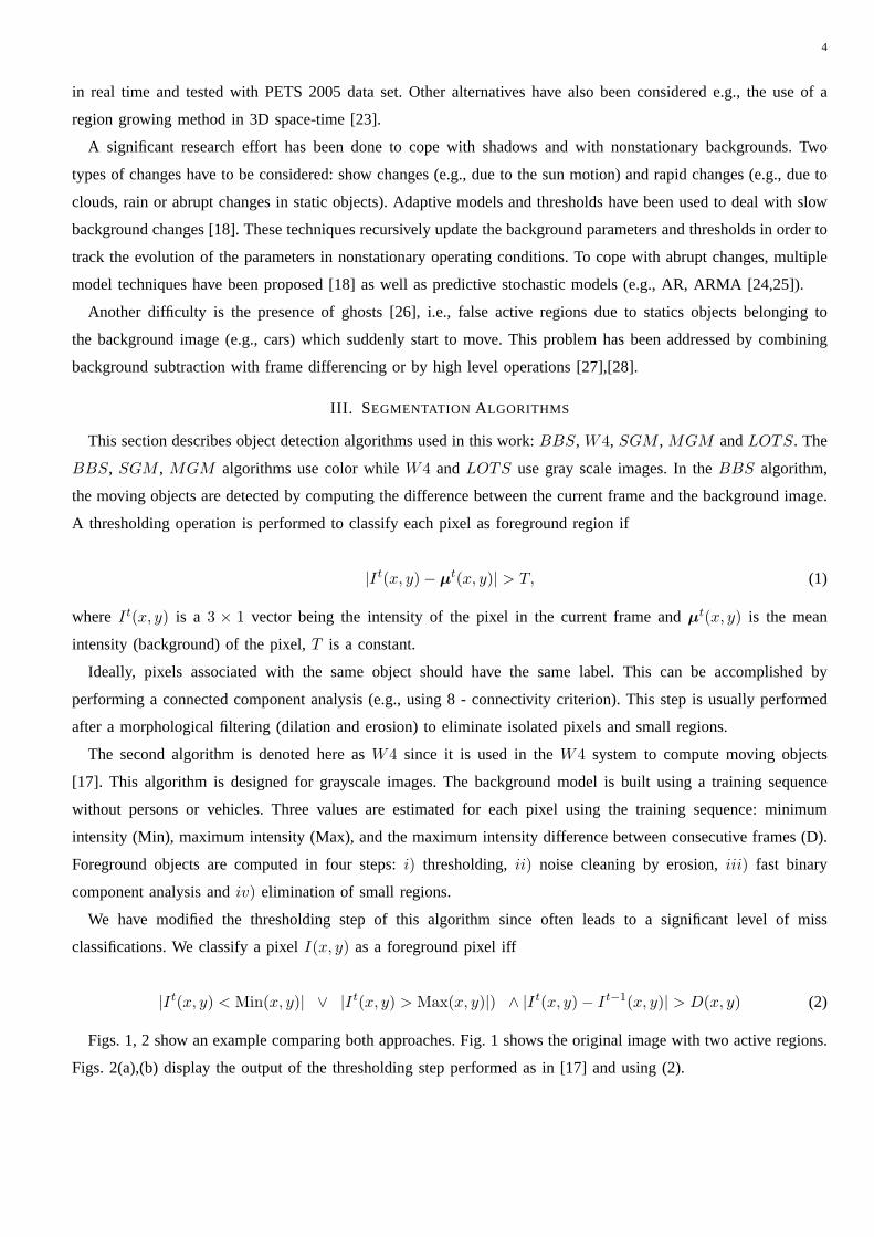
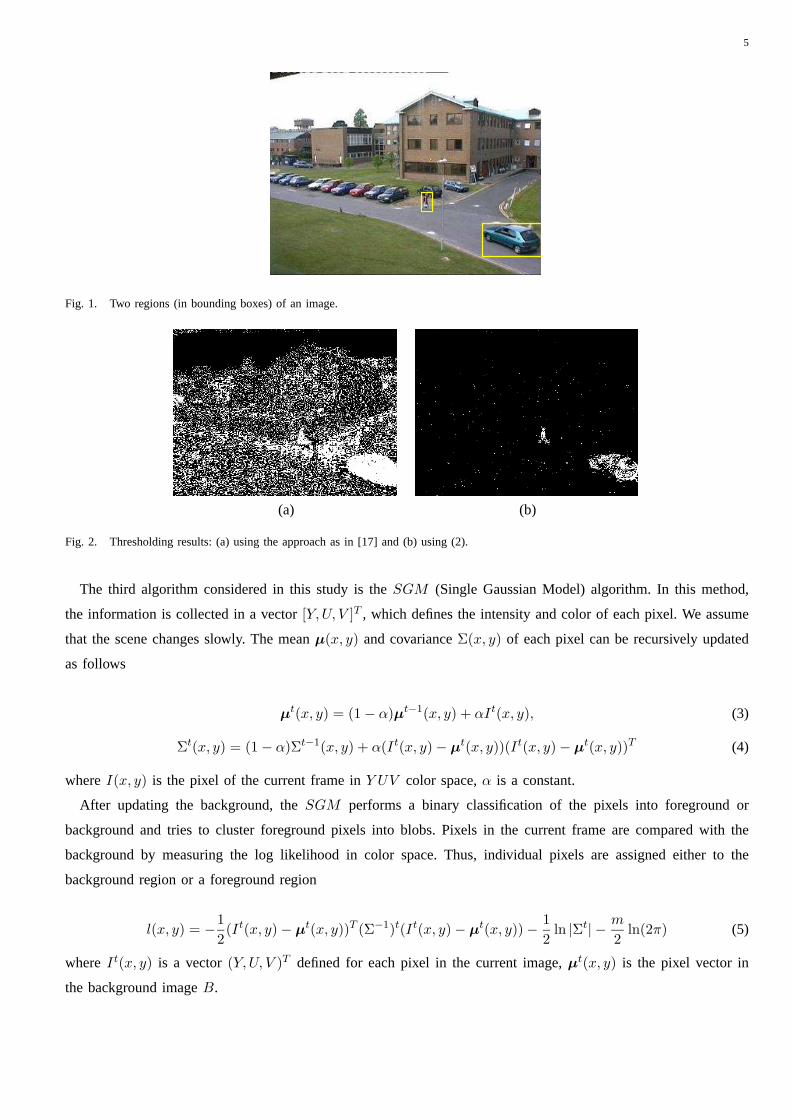
Figs. 1, 2 show an example comparing both approaches. Fig. 1 shows the original image with two active regions.
Figs. 2(a),(b) display the output of the thresholding step performed as in [17] and using (2).
5
Fig. 1. Two regions (in bounding boxes) of an image.
(a) (b)
Fig. 2. Thresholding results: (a) using the approach as in [17] and (b)using (2).
The third algorithm considered in this study is theSGM (Single Gaussian Model) algorithm. In this method,
the information is collected in a vector[Y, U, V ]T , which defines the intensity and color of each pixel. We assume
that the scene changes slowly. The meanµ(x, y) and covarianceΣ(x, y) of each pixel can be recursively updated
as follows
µt(x, y) = (1− α)µt−1(x, y) + αIt(x, y), (3)
Σt(x, y) = (1− α)Σt−1(x, y) + α(It(x, y)− µt(x, y))(It(x, y)− µ
t(x, y))T (4)
whereI(x, y) is the pixel of the current frame inY UV color space,α is a constant.
After updating the background, theSGM performs a binary classification of the pixels into foreground or
background and tries to cluster foreground pixels into blobs. Pixels in the current frame are compared with the
background by measuring the log likelihood in color space. Thus, individual pixels are assigned either to the
background region or a foreground region
l(x, y) = −1
2(It(x, y)− µ
t(x, y))T (Σ−1)t(It(x, y)− µt(x, y))−
1
2ln |Σt| −
m
2ln(2π) (5)
whereIt(x, y) is a vector(Y, U, V )T defined for each pixel in the current image,µt(x, y) is the pixel vector in
the background imageB.
6
If a small likelihood is computed using (5), the pixel is classified as active. Otherwise, it is classified as
background.
The fourth algorithm (MGM ) models each pixelI(x) = I(x, y) as a mixture ofN(N = 3) Gaussians distributions,
i.e.
p(I(x)) =
N∑
k=1
ωkN (I(x), µk(x), Σk(x)), (6)
whereN (I(x), µk(x), Σk(x)) is a multivariate normal distribution andωk is the weight ofkth normal,
N (I(x), µk(x), Σk(x)) = c exp{
−1
2
(
I(x)− µk(x))T
Σ−1k (x)
(
I(x)− µk(x))}
. (7)
with c = 1
(2π)n/2|Σk|1
2
. Note that each pixelI(x) is a3×1 vector with three component colors (red, green and blue),
i.e., I(x) = [I(x)RI(x)GI(x)B]T . To avoid an excessive computational cost, the covariance matrix is assumed to
be diagonal [2].
The mixture model is dynamically updated. Each pixel is updated as follows:i) The algorithm checks if each
incoming pixel valuex can be ascribed to a given mode of the mixture, this is the match operation.ii) If the pixel
value occurs inside the confidence interval with+2.5 standard deviation, a match event is verified. The parameters
of the corresponding distributions (matched distributions) for that pixel are updated according to
µtk(x) = (1− λt
k)µt−1k (x) + λt
kIt(x) (8)
Σtk(x) = (1− λt
k)Σt−1k (x) + λt
k(It(x)− µ
tk(x))(It(x)− µ
tk(x))T (9)
where
λtk = αN (It(x), µt−1
k (x), Σt−1k (x)) (10)
The weights are updated by
ωtk = (1− α)ωt−1
k + α(M tk), with M t
k =
1 matched models
0 remaining models(11)
α is the learning rate. The non match components of the mixture are not modified. If none of the existing components
match the pixel value, the least probable distribution is replaced by a normal distribution with mean equal to the
current value, a large covariance and small weight.iii) The next step is to order the distributions in the descending
order of ω/σ. This criterion favours distributions which have more weight (most supporting evidence) and less
variance (less uncertainty).iv) Finally the algorithm models each pixel as the sum of the corresponding updated
distributions. The firstB Gaussian modes are used to represent the background, while the remaining modes are
considered as foreground distributions.B is chosen as follows:B is the smallest integer such that
B∑
k=1
ωk > T (12)
whereT is a threshold that accounts for a certain quantity of data that should belong to the background.
7
The fifth algorithm [18] is tailored for the detection of non cooperative targets (e.g., snipers) under non stationary
environments. The algorithm uses two gray level background imagesB1, B2. This allows the algorithm to cope with
intensity variations due to noise or fluttering objects, moving in the scene. The background images are initialized
using a set ofT consecutive frames, without active objects
B1(x, y) = min{It(x, y), t = 1, . . . , T} (13)
B2(x, y) = max{It(x, y), t = 1, . . . , T} (14)
wheret ∈ {1, 2, . . . , T} denotes the time instant.
In this method, targets are detected by using two thresholds(TL, TH ) followed by aquasi-connected components
(QCC) analysis. These thresholds are initialized using the difference between the background images
TL(x, y) = |B1(x, y)−B2(x, y) |+ cU (15)
TH(x, y) = TL(x, y) + cS (16)
where,cU andcS ∈ [0, 255] are constants specified by the user.
We compute the difference between each pixel and the closestbackground image. If the difference exceeds a
low thresholdTL, i.e.,
mini|It(x, y)−Bt
i(x, y)| > TL(x, y) (17)
the pixel is considered as active. A target is a set of connected active pixels such that a subset of them verifies
mini|It(x, y)−Bt
i(x, y)| > TH(x, y) (18)
whereTH(x, y) ia a high threshold. The low and high thresholdsT tL(x, y), T t
H(x, y) as well as the background
images,Bti(x, y), i = 1, 2 are recursively updated in a fully automatic way (see [18] for details).
IV. PROPOSEDFRAMEWORK
In order to evaluate the performance of object detection algorithms we propose a framework which is based on
the following principles:
• A set sequences is selected for testing and all the moving objects are detected using an automatic procedure
and manually corrected if necessary to obtain the ground truth. This is performed one frame per second.
• The output of the automatic detector is compared with the ground truth.
• The errors are detected and classified in one of the following classes: correct detections, detections failures,
splits, merges, split/merges and false alarms.
• A set of statistics (mean, standard deviation) are computedfor each type of error.
To perform the first step we made a user friendly interface which allows the user to define the foreground regions
in the test sequence in a semi-automatic way. Fig. 3 shows the interface used to generate the ground truth. A set
of frames is extracted from the test sequence (one per second). An automatic object detection algorithm is then
used to provide a tentative segmentation of the test images.Finally, the automatic segmentation is corrected by the

8
user, by merging, splitting, removing or creating active regions. Typically the boundary of the object is detected
with a two pixel accuracy. Multiple segmentations of the video data are generated every time there is an ambiguous
situation i.e., two close regions which are almost overlapping. This problem is discussed in section IV-D.
In the case depicted in the Fig. 3, there are four active regions: a car, a lorry and two groups of persons. The
segmentation algorithm also detects regions due to lighting changes, leading to a number of false alarms (four). The
user can easily edit the image by adding, removing, checkingthe operations, thus providing a correct segmentation.
In Fig. 3 we can see an example where the user progressively removes the regions which do not belong to the
object of interest. The final segmentation is shown at the bottom images.
Fig. 3. User interface used to create the ground truth from the automatic segmentation of the video images.
The test images are used to evaluate the performance of objectdetection algorithms. In order to compare the
output of the algorithm with the ground truth segmentation,a region matching procedure is adopted which allows
to establish a correspondence between the detected objectsand the ground truth. Several cases are considered:
1) Correct Detection (CD) or 1-1 match: the detected region matches one and only one region.
2) False Alarm (FA): the detected region has no correspondence.
3) Detection Failure (DF): the ground truth region has no correspondence.
4) Merge Region (M): the detected region is associated to several ground truth regions.
5) Split Region (S): the ground truth region is associated to several detected regions.
6) Split-Merge Region (SM): when the conditions pointed in 4, 5 are simultaneously satisfied.
A. Region Matching
Object matching is performed by computing a binary correspondence matrixCt which defines the correspondence
between the active regions in a pair of images. Let us assume that we have N ground truth regionsRi and M
detected regionsRj . Under these conditionsCt is a N ×M matrix, defined as follows
9
Ct(i, j) =
1 if♯(Ri ∩Rj)
♯(Ri ∪Rj)> T
∀i∈{1,...,N},j∈{1,...,M}
0 if♯(Ri ∩Rj)
♯(Ri ∪Rj)< T
(19)
whereT is the threshold which accounts for the overlap requirement. It is also useful to add the number of ones
in each line or column, defining two auxiliary vectors
L(i) =M∑
j=1
C(i, j) i ∈ {1, . . . , N} (20)
C(j) =N∑
i=1
C(i, j) j ∈ {1, . . . , M} (21)
When we associate ground truth regions with detected regions six cases can occur: zero-to-one, one-to-zero,
one-to-one, many-to-one, one-to-many, many-to-many associations. These correspond to false alarm, misdetection,
correct detection, merge, split and split-merge.
Detected regionsRj are classified according to the following rules
CD ∃i : L(i) = C(j) = 1 ∧ C(i, j) = 1M ∃i : C(j) > 1 ∧ C(i, j) = 1S ∃i : L(i) > 1 ∧ C(i, j) = 1SM ∃i : L(i) > 1 ∧ C(j) > 1 ∧ C(i, j) = 1FA ∃i : C(j) = 0
(22)
Detection failures (DF ) associated to the ground truth regionRi occurs ifL(i) = 0.
The two last situations (FA, DF) in (22) occur whenever empty columns or lines in matrixC are observed.
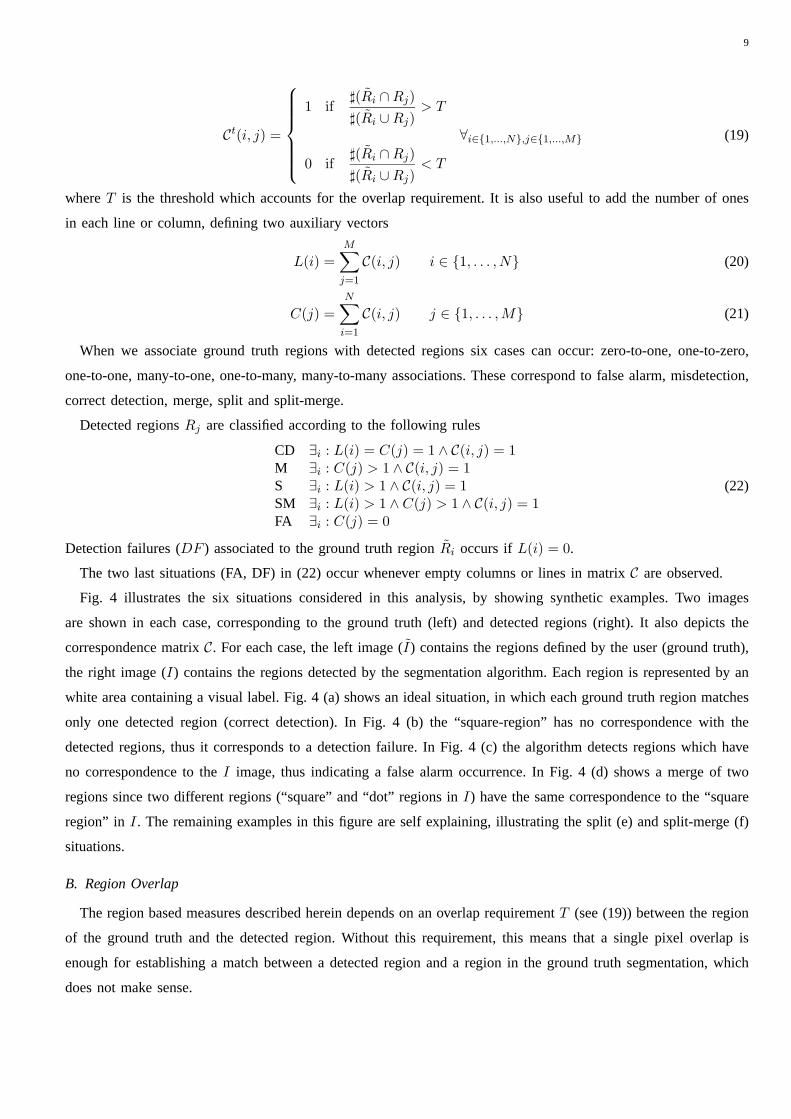
Fig. 4 illustrates the six situations considered in this analysis, by showing synthetic examples. Two images
are shown in each case, corresponding to the ground truth (left) and detected regions (right). It also depicts the
correspondence matrixC. For each case, the left image (I) contains the regions defined by the user (ground truth),
the right image (I) contains the regions detected by the segmentation algorithm. Each region is represented by an
white area containing a visual label. Fig. 4 (a) shows an idealsituation, in which each ground truth region matches
only one detected region (correct detection). In Fig. 4 (b) the “square-region” has no correspondence with the
detected regions, thus it corresponds to a detection failure. In Fig. 4 (c) the algorithm detects regions which have
no correspondence to theI image, thus indicating a false alarm occurrence. In Fig. 4 (d)shows a merge of two
regions since two different regions (“square” and “dot” regions in I) have the same correspondence to the “square
region” in I. The remaining examples in this figure are self explaining, illustrating the split (e) and split-merge (f)
situations.
B. Region Overlap
The region based measures described herein depends on an overlap requirementT (see (19)) between the region
of the ground truth and the detected region. Without this requirement, this means that a single pixel overlap is
enough for establishing a match between a detected region and a region in the ground truth segmentation, which
does not make sense.

10
A match is determined to occur if the overlap is at least as bigas the Overlap Requirement. The bigger the overlap
requirement, the more the boxes are required to overlap hence performance usually declines as the requirement
reaches 100%. In this work we use a overlap requirement ofT = 10%.
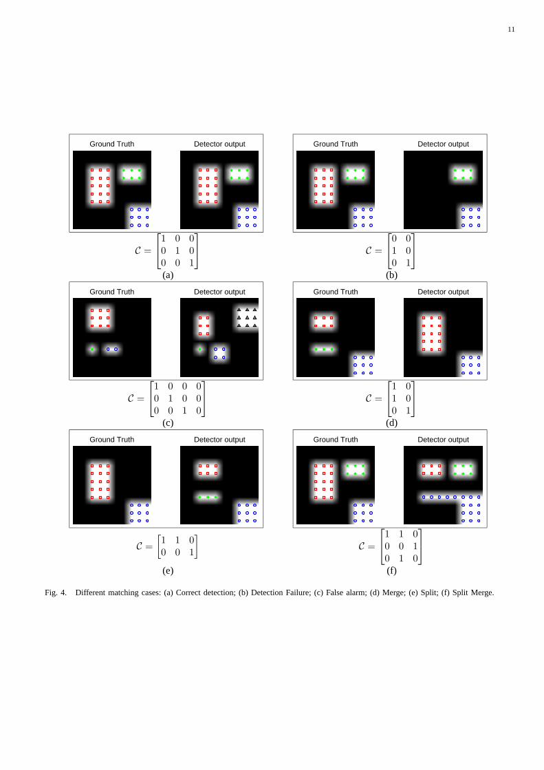
Fig. 5 illustrates the association matrices in two differentcases considering an overlap requirement ofT = 20%.
It can be seen that in Fig. 5(a) the region in the ground truth (“circle” region) is not represented by any detected
region since the overlap is below the overlap requirement, leading to a detection failure. If we increase the overlap
between these two regions (see Fig. 5(b)) we see that now we have a correct detection (second line, second column
of C). Finally it is illustrated a situation where two detection failures (in Fig. 5 (c)) become a split (in Fig. 5 (d))
if we increase the overlap among these regions.
C. Area Matching
The match between pairs of the two regions (ground truth/ automatically detected) is also considered to measure
the performance of the algorithms. The higher is the percentage of the match size, the better are the active regions
produced by the algorithm. This is done for all the correctly detected regions. The match metric is defined by
M(i) = ♯(Ri∩Rj)
♯(Ri∪Rj), wherej is the index of the corresponding detected region. The metricM is the area of the
overlap normalized by the total area of the object. The average of M(i) in a video sequence will be used to
characterize the performance of the detector.
11
Ground Truth Detector output Ground Truth Detector output
C =
1 0 00 1 00 0 1
C =
0 01 00 1
(a) (b)
Ground Truth Detector output Ground Truth Detector output
C =
1 0 0 00 1 0 00 0 1 0
C =
1 01 00 1
(c) (d)
Ground Truth Detector output Ground Truth Detector output
C =
[1 1 00 0 1
]
C =
1 1 00 0 10 1 0
(e) (f)
Fig. 4. Different matching cases: (a) Correct detection; (b) DetectionFailure; (c) False alarm; (d) Merge; (e) Split; (f) Split Merge.
12
Ground Truth Detector output Ground Truth Detector output
C =
[1 0 00 0 0
]
C =
[1 0 00 1 0
]
(a) (b)
Ground Truth Detector output Ground Truth Detector output
C =
[1 0 00 0 0
]
C =
[1 0 00 1 1
]
(c) (d)
Fig. 5. Matching cases with an overlap requirement ofT = 20%. Detection failure (overlap< T) (a) Correct detection (overlap> T) (b);two detection failures (overlap< T) (c) and split (overlap> T) (d).

13
D. Multiple Interpretations
Sometimes the segmentation procedure is subjective, since each active region may contain several objects and
it is not always easy to determine if it is a single connected region or several disjoint regions. For instance, Fig.
6 (a) shows an input image and a manual segmentation. Three active regions were considered: person, lorry and
group of people. Fig. 6 (b) shows the segmentation results provided by theSGM algorithm. This algorithm splits
the group into three individuals which can also be considered as a valid solution since there is very little overlap.
This segmentation should be considered as an alternative ground truth. All these situations should not penalize the
performance of the algorithm. On the contrary, situations such as the ones depicted in Fig. 7 should be considered
as errors. Fig. 7 (a) shows the ground truth and in Fig. 7 (b) the segmentation provided by theW4 algorithm. In
this situation the algorithm makes a wrong split of the vehicle.
(a) (b)
Fig. 6. Correct split example: (a) supervised segmentation, (b)SGM segmentation.
(a) (b)
Fig. 7. Wrong split example: (a) supervised segmentation, (b)W4 segmentation.
Since we do not know how the algorithm behaves in terms of merging or splitting, every possible combinations
within elements, belonging to a group, must be taken into account. For instance, another ambiguous situation is
depicted in Fig. 8, where it is shown the segmentation resultsof the SGM method. Here, we see that the same
algorithm provides different segmentations (both can be considered as correct) on the same group in different

14
instants. This suggests the use of multiple interpretationsfor the segmentation. To accomplish this the evaluation
setup takes into account all possible merges of single regions belonging to the same group whenever multiple
interpretations should be considered in a group, i.e., whenthere is a small overlap among the group members.
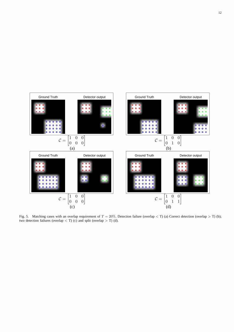
The number of merges depends on the relative position of single regions. Fig. 9 shows two examples of different
merged regions groups with three objects ABC (each one representing a person in the group). In the first example
(Fig. 9 (a)) four interpretations are considered: all the objects are separated, they are all merged in a single active
region or AB (BC) are linked and the other is isolated. In the second example an addition interpretation is added
since A can be linked with C.
Instead of asking the user to identify all the possible merges in an ambiguous situation, an algorithm is used to
generate all the valid interpretations in two steps. First weassign all the possible labels sequences to the group
regions. If the same label is assigned to two different regions, these regions are considered as merged. Equation
(23)(a) shows the labelling matrixM for the example of Fig. 9 (a). Each row corresponds to a different labelling
assignment. The elementMij denotes the label of thejth region in theith labelling configuration. The second
step checks if the merged regions are close to each other and if there is another region in the middle. The invalid
labelling configuration are removed from the matrixM . The output of this step for the example of Fig. 9 (a) is
in equation (23)(b). The labelling sequence121 is discarded since region 2 is between region 1 and 3. Therefore,
regions 1, 3 cannot be merged. In the case of the Fig. 9 (b) all the configurations are possible (M = MFINAL). A
detailed description of the labelling method is included inappendix VII-A.
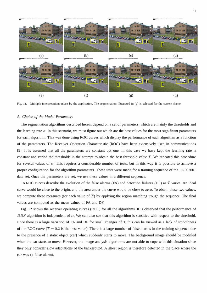
Figs. 10,11 illustrate the generation of the valid interpretations. Fig. 10 (a) shows the input frame, Fig. 10 (b)
shows the hand segmented image, where the user specifies all the objects (three objects must be provided separately
in the group of persons) and Fig. 10 (c) illustrates the outputof the SGM . Fig. 11 shows all possible merges of
individual regions. All of them are considered as correct. Remain to know which segmentation should be selected
to appraise the performance. In this paper we choose the bestsegmentation, which is the one that provides the
highest number of correct detections. In the present example the segmentation illustrated in Fig. 11 (g) is selected.
In this way we overcome the segmentation ambiguities that may appear without penalizing the algorithm. This is
the most complex situation which occurs in the video sequences used in this paper.
Fig. 8. Two different segmentations, provided bySGM method on the same group taken at different time instants.
15
(a) (b)
Fig. 9. Regions linking procedure with three objects A B C (from left to right). The same number of foreground regions may have differentinterpretations: three possible configurations (a), or four configurations (b). Each color represent a different region.
M =
1 1 11 1 21 2 11 2 21 2 3
(a)
MFINAL =
1 1 11 1 2
1 2 21 2 3
(b)
(23)
(a) (b) (c)
Fig. 10. Input frame (a), segmented image by the user (b), output ofSGM (c).
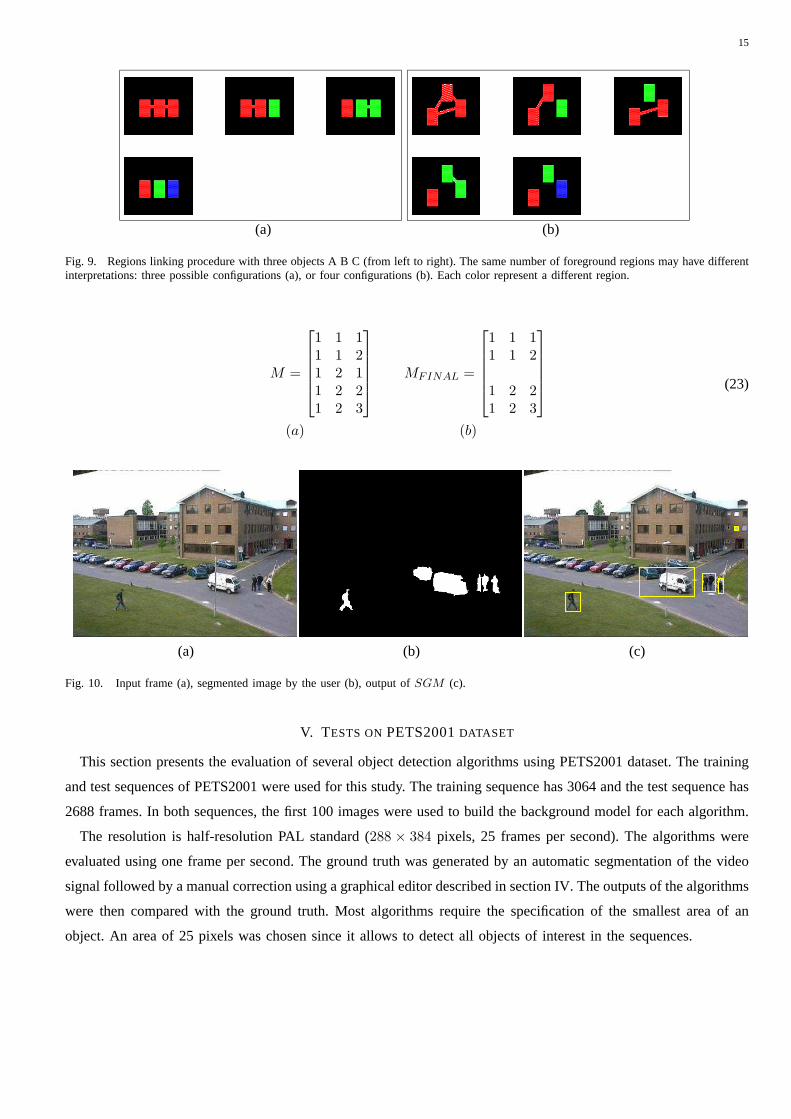
V. TESTS ONPETS2001DATASET
This section presents the evaluation of several object detection algorithms using PETS2001 dataset. The training
and test sequences of PETS2001 were used for this study. The training sequence has 3064 and the test sequence has
2688 frames. In both sequences, the first 100 images were used to build the background model for each algorithm.
The resolution is half-resolution PAL standard (288 × 384 pixels, 25 frames per second). The algorithms were
evaluated using one frame per second. The ground truth was generated by an automatic segmentation of the video
signal followed by a manual correction using a graphical editor described in section IV. The outputs of the algorithms
were then compared with the ground truth. Most algorithms require the specification of the smallest area of an
object. An area of 25 pixels was chosen since it allows to detect all objects of interest in the sequences.
16
(a) (b) (c) (d)
(e) (f) (g) (h)
Fig. 11. Multiple interpretations given by the application. The segmentation illustrated in (g) is selected for the current frame.
A. Choice of the Model Parameters
The segmentation algorithms described herein depend on a setof parameters, which are mainly the thresholds and
the learning rateα. In this scenario, we must figure out which are the best values for the most significant parameters
for each algorithm. This was done using ROC curves which display the performance of each algorithm as a function
of the parameters. The Receiver Operation Characteristic (ROC) have been extensively used in communications
[9]. It is assumed that all the parameters are constant but one. In this case we have kept the learning rateα
constant and varied the thresholds in the attempt to obtain the best threshold valueT . We repeated this procedure
for several values ofα. This requires a considerable number of tests, but in this wayit is possible to achieve a
proper configuration for the algorithm parameters. These tests were made for a training sequence of the PETS2001
data set. Once the parameters are set, we use these values in adifferent sequence.
To ROC curves describe the evolution of the false alarms (FA)and detection failures (DF) asT varies. An ideal
curve would be close to the origin, and the area under the curve would be close to zero. To obtain these two values,
we compute these measures (for each value ofT ) by applying the region matching trough the sequence. The final
values are computed as the mean values of FA and DF.
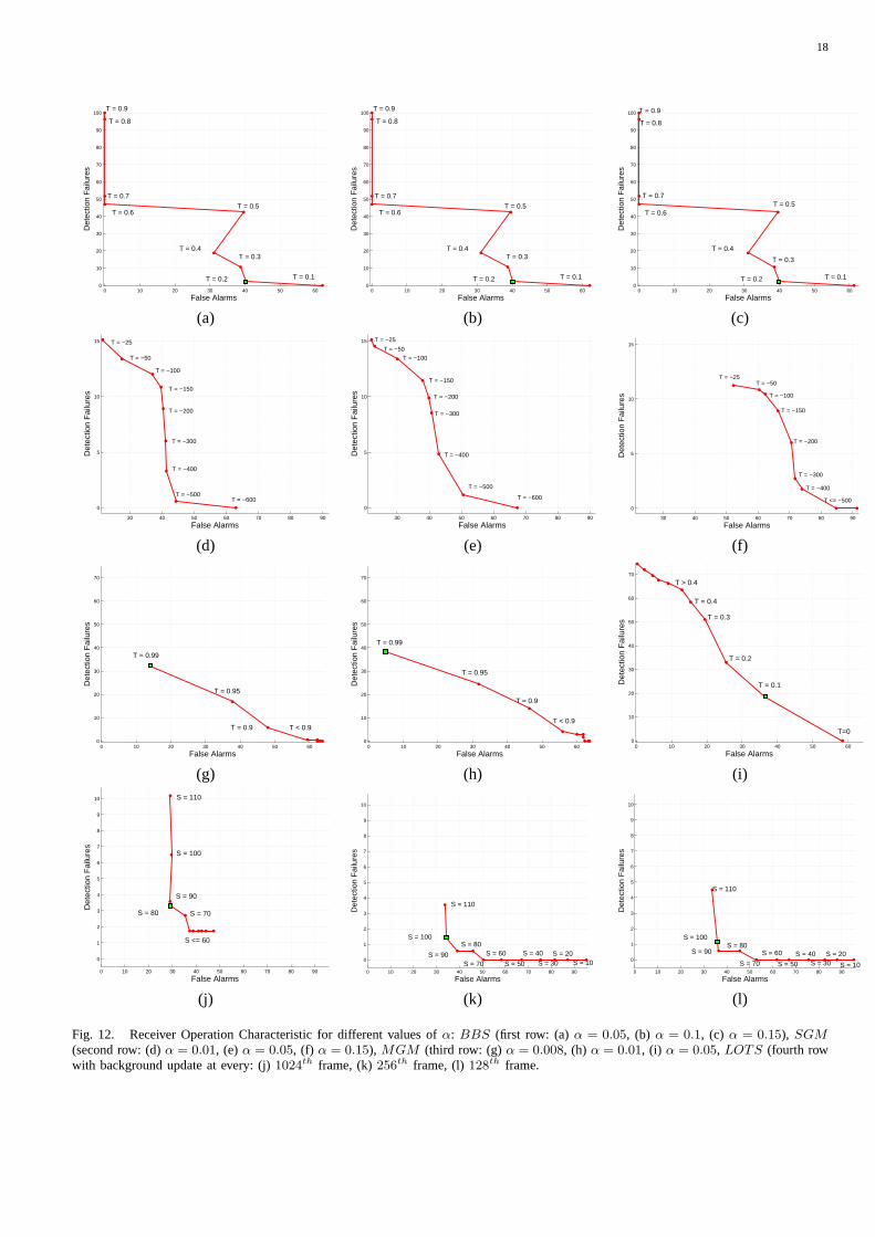
Fig. 12 shows the receiver operating curves (ROC) for all the algorithms. It is observed that the performance of
BBS algorithm is independent ofα. We can also see that this algorithm is sensitive with respect to the threshold,
since there is a large variation of FA and DF for small changesof T, this can be viewed as a lack of smoothness
of the ROC curve (T = 0.2 is the best value). There is a large number of false alarms in the training sequence due
to the presence of a static object (car) which suddenly starts to move. The background image should be modified
when the car starts to move. However, the image analysis algorithms are not able to cope with this situation since
they only consider slow adaptations of the background. A ghost region is therefore detected in the place where the
car was (a false alarm).
17
The second row of the Fig. 12 shows the ROC curves of theSGM method, for three values ofα (0.01, 0.05, 0.15).
This method is more robust than theBBS algorithm with respect to the threshold. We see that for−400 < T <
−150, andα = 0.01, α = 0.05 we get similar FA rates and a small variation of DF. We choseα = 0.05, T = −400.
The third row show the results of theMGM method. The best performances are obtained forα < 0.05 (first
and second column). The best value of theα parameter isα = 0.008. In fact, we observe the best performances
for α ≤ 0.01. We notice that the algorithm strongly depends on the value of T , since for small variations ofT
there are significant changes of FA and DF. The ROC curve suggestthat it is acceptable to chooseT > 0.9.
The fourth row shows the results of theLOTS algorithm for a variation of the sensitivity from10% to 110%.
As discussed in [29] we use a smallα parameter. For the sake of computational burden,LOTS does not update
the background image in every single frame. This algorithm decreases the background update rate which takes
place in periods ofN frames. For instance an effective integration factorα = 0.0003 is achieved by adding
approximately 113 of the current frame to the background in every256th frame, or 1
6.5 in every 512th frame.
Remark thatBt = Bt−1 + αDt, with Dt = It −Bt. In our case we have used intervals of1024 (Fig. 12 (j)) 256
(Fig. 12 (k)) 128 (Fig. 12 (l)), being the best results achieved in the first case.The latter two cases Fig.(12) (k),
(l) present a right shift in relation to (j), meaning that in these cases one obtains a large number of false alarms.
From this study we conclude that the best ROC curves are the curves associated withLOTS andSGM since
they have the smallest area under the curve.
18
0 10 20 30 40 50 600
10
20
30
40
50
60
70
80
90
100
False Alarms
Det
ectio
n F
ailu
res
T = 0.9
T = 0.8
T = 0.7
T = 0.6 T = 0.5
T = 0.4 T = 0.3
T = 0.2 T = 0.1
0 10 20 30 40 50 600
10
20
30
40
50
60
70
80
90
100
False Alarms
Det
ectio
n F
ailu
res
T = 0.9
T = 0.8
T = 0.7
T = 0.6 T = 0.5
T = 0.4 T = 0.3
T = 0.2 T = 0.1
0 10 20 30 40 50 600
10
20
30
40
50
60
70
80
90
100
False Alarms
Det
ectio
n F
ailu
res
T = 0.9
T = 0.8
T = 0.7
T = 0.6 T = 0.5
T = 0.4
T = 0.3
T = 0.2 T = 0.1
(a) (b) (c)
30 40 50 60 70 80 90
0
5
10
15
False Alarms
Det
ectio
n F
ailu
res
T = −600 T = −500
T = −400
T = −300
T = −200
T = −150
T = −100
T = −50
T = −25
30 40 50 60 70 80 90
0
5
10
15
False Alarms
Det
ectio
n F
ailu
res
T = −600
T = −500
T = −400
T = −300
T = −200
T = −150
T = −100
T = −50
T = −25
30 40 50 60 70 80 90
0
5
10
15
False Alarms
Det
ectio
n F
ailu
res
T = −25 T = −50
T = −100
T = −150
T = −200
T = −300
T = −400
T <= −500
(d) (e) (f)
0 10 20 30 40 50 600
10
20
30
40
50
60
70
False Alarms
Det
ectio
n F
ailu
res
T = 0.99
T = 0.95
T = 0.9 T < 0.9
0 10 20 30 40 50 600
10
20
30
40
50
60
70
False Alarms
Det
ectio
n F
ailu
res
T = 0.99
T = 0.95
T = 0.9
T < 0.9
0 10 20 30 40 50 600
10
20
30
40
50
60
70
False Alarms
Det
ectio
n F
ailu
res
T=0
T = 0.1
T = 0.2
T = 0.3
T = 0.4
T > 0.4
(g) (h) (i)
0 10 20 30 40 50 60 70 80 90
0
1
2
3
4
5
6
7
8
9
10
False Alarms
Det
ectio
n F
ailu
res
S = 110
S = 100
S = 90
S = 80 S = 70
S <= 60
0 10 20 30 40 50 60 70 80 90
0
1
2
3
4
5
6
7
8
9
10
False Alarms
Det
ectio
n F
ailu
res
S = 110
S = 100
S = 90
S = 80
S = 70
S = 60
S = 50
S = 40
S = 30 S = 20
S = 10 0 10 20 30 40 50 60 70 80 90
0
1
2
3
4
5
6
7
8
9
10
False Alarms
Det
ectio
n F
ailu
res
S = 110
S = 100
S = 90 S = 80
S = 70
S = 60
S = 50
S = 40 S = 30
S = 20
S = 10
(j) (k) (l)
Fig. 12. Receiver Operation Characteristic for different values ofα: BBS (first row: (a) α = 0.05, (b) α = 0.1, (c) α = 0.15), SGM
(second row: (d)α = 0.01, (e) α = 0.05, (f) α = 0.15), MGM (third row: (g)α = 0.008, (h) α = 0.01, (i) α = 0.05, LOTS (fourth rowwith background update at every: (j)1024th frame, (k)256th frame, (l)128th frame.
19
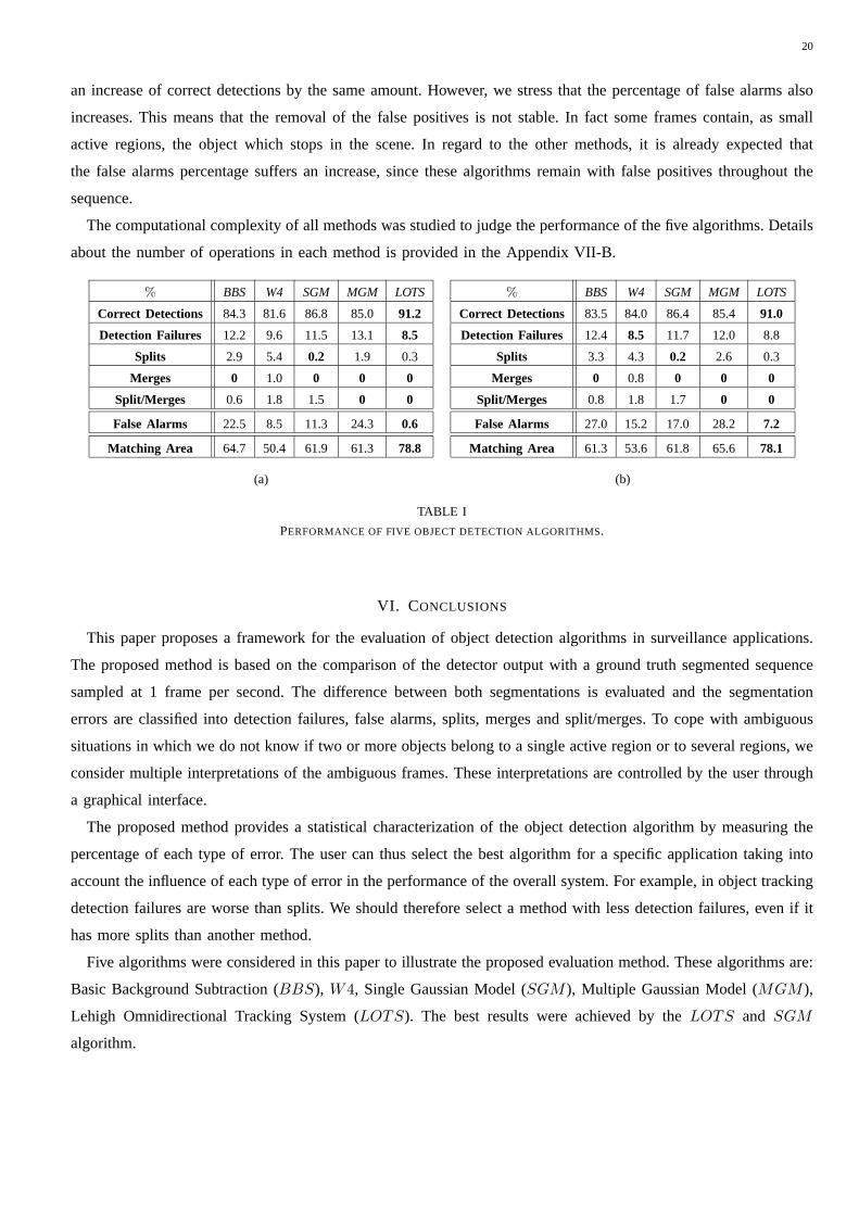
B. Performance Evaluation
Table I (a),(b) shows the results obtained in the test sequence using the parameters selected in the previous
study. The percentage of correct detections, detection failures, splits, merges and split-merges were obtained by
normalizing the number of each type of event by the total number of moving objects in the image. Their sum is
100%. The percentage of false alarms is defined by normalizing the number of false alarms by the total number of
detected objects. It is therefore a number in the range0− 100%.
Each algorithm is characterized in terms of correct detections, detection failures, number of splits, merges and
split/merges false alarms as well as matching area.
Two types of ground truth were used. They correspond to different interpretations of static objects. If a moving
object stops and remains still it is considered an active region in the first case (Table I (a)) and it is integrated in
the background after one minute in the second case (Table I (b)). For example, if a car stops in front of the camera
it will always be an active region in the first case. In the second case it will be ignored after one minute.
Let us consider the first case. The results are shown in Table I (a). In terms of correct detections, the best results
are achieved by theLOTS (91.2%) algorithm followed bySGM (86.8%).
Concerning the detection failures, theLOTS (8.5%) followed by W4 (9.6%) outperforms all the others. The
worst results are obtained byMGM (13.1%). This is somewhat surprising sinceMGM method, based on the
use of multiple Gaussians per pixel, performs worse than theSGM method based on a single Gaussian. We will
discuss this issue bellow. TheW4 has the highest percentage of splits and theBBS, MGM methods tend to split
the regions as well. The performance of the methods in terms ofregion merging is excellent: very few merges are
observed in the segmented data. However, some methods tend to produce split/merges errors (e.g.,W4, SGM and
BBS). The LOTS andMGM algorithm have the best score in terms of split/merge errors.
Let us now consider the false alarms (false positives). TheLOTS (0.6%) is the best and theMGM andBBS
are the worst. TheLOTS, W4 andSGM methods are much better than the others in terms of false alarms.
TheLOTS has the best tradeoff between CD and FA. Although theW4 produces many splits (splits can often be
overcome in tracking applications since the region matching algorithms are able to track the active regions though
they are split). TheLOTS algorithm has the best performance if all the errors are equally important.
In terms of matching area theLOTS exhibit the best value in both situations.
In this study, the performance of theMGM method, based on mixtures of Gaussians is unexpectedly low.
During the experiments we have observed the following:i) when the object undergoes a slow motion and stops,
the algorithm ceases to detect the object after a small period of time; ii) when an object enters the scene it is not
well detected during a few frames since the Gaussian modes have to adapt to this case.
This situation justify the percentage of the splits in both Tables. In fact, when a moving object stops, theMGM
starts to split the region until it disappears, becoming part of the background. Objects entering into the scene will
cause some detection failures (during the first frames) and splits, when theMGM method starts to separate the
foreground region from the background.
Comparing the results in Table I (a) and (b) we can see that theperformance of theMGM is improved. The
detection failures are reduced, meaning that the stopped car is correctly integrated in the background. This produces
20
an increase of correct detections by the same amount. However, we stress that the percentage of false alarms also
increases. This means that the removal of the false positivesis not stable. In fact some frames contain, as small
active regions, the object which stops in the scene. In regard to the other methods, it is already expected that
the false alarms percentage suffers an increase, since these algorithms remain with false positives throughout the
sequence.
The computational complexity of all methods was studied to judge the performance of the five algorithms. Details
about the number of operations in each method is provided in the Appendix VII-B.
% BBS W4 SGM MGM LOTS
Correct Detections 84.3 81.6 86.8 85.0 91.2
Detection Failures 12.2 9.6 11.5 13.1 8.5
Splits 2.9 5.4 0.2 1.9 0.3
Merges 0 1.0 0 0 0
Split/Merges 0.6 1.8 1.5 0 0
False Alarms 22.5 8.5 11.3 24.3 0.6
Matching Area 64.7 50.4 61.9 61.3 78.8
% BBS W4 SGM MGM LOTS
Correct Detections 83.5 84.0 86.4 85.4 91.0
Detection Failures 12.4 8.5 11.7 12.0 8.8
Splits 3.3 4.3 0.2 2.6 0.3
Merges 0 0.8 0 0 0
Split/Merges 0.8 1.8 1.7 0 0
False Alarms 27.0 15.2 17.0 28.2 7.2
Matching Area 61.3 53.6 61.8 65.6 78.1
(a) (b)
TABLE I
PERFORMANCE OF FIVE OBJECT DETECTION ALGORITHMS.
VI. CONCLUSIONS
This paper proposes a framework for the evaluation of object detection algorithms in surveillance applications.
The proposed method is based on the comparison of the detectoroutput with a ground truth segmented sequence
sampled at 1 frame per second. The difference between both segmentations is evaluated and the segmentation
errors are classified into detection failures, false alarms,splits, merges and split/merges. To cope with ambiguous
situations in which we do not know if two or more objects belong to a single active region or to several regions, we
consider multiple interpretations of the ambiguous frames. These interpretations are controlled by the user through
a graphical interface.
The proposed method provides a statistical characterization of the object detection algorithm by measuring the
percentage of each type of error. The user can thus select the best algorithm for a specific application taking into
account the influence of each type of error in the performance of the overall system. For example, in object tracking
detection failures are worse than splits. We should therefore select a method with less detection failures, even if it
has more splits than another method.
Five algorithms were considered in this paper to illustrate the proposed evaluation method. These algorithms are:
Basic Background Subtraction (BBS), W4, Single Gaussian Model (SGM ), Multiple Gaussian Model (MGM ),
Lehigh Omnidirectional Tracking System (LOTS). The best results were achieved by theLOTS and SGM
algorithm.

21
Acknowledgement: We are very grateful to the three anonymous reviewers for their useful comments and
suggestions. We also thank R. Oliveira and P. Ribeiro for kindly provide the code ofLOTS detector.
22
VII. A PPENDIX
A. Merge Regions Algorithm
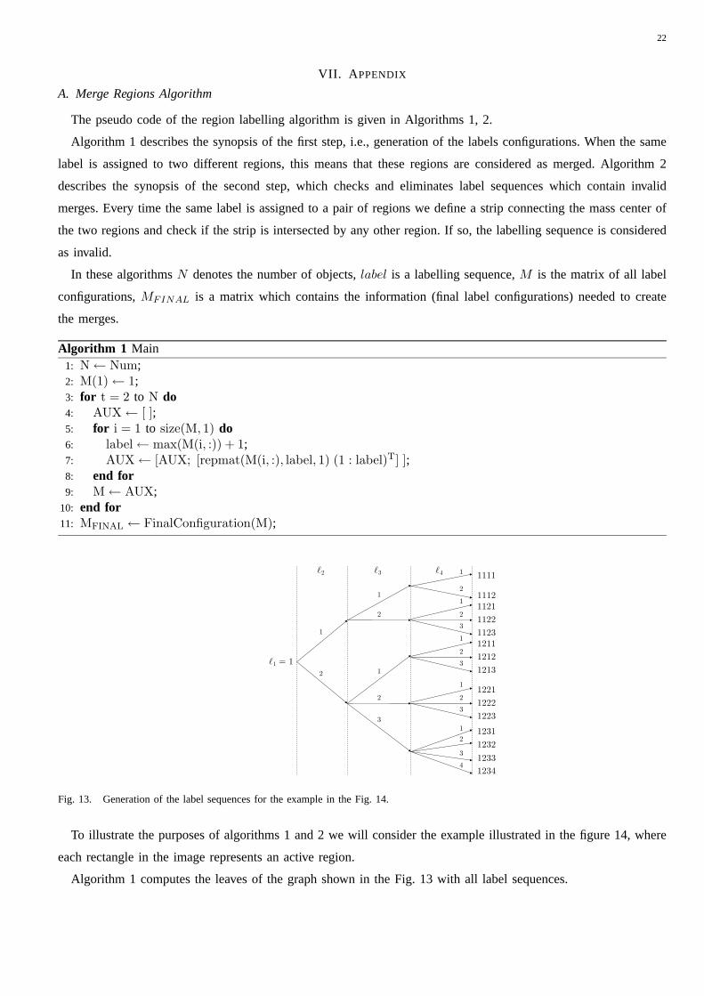
The pseudo code of the region labelling algorithm is given in Algorithms 1, 2.
Algorithm 1 describes the synopsis of the first step, i.e., generation of the labels configurations. When the same
label is assigned to two different regions, this means that these regions are considered as merged. Algorithm 2
describes the synopsis of the second step, which checks and eliminates label sequences which contain invalid
merges. Every time the same label is assigned to a pair of regions we define a strip connecting the mass center of
the two regions and check if the strip is intersected by any other region. If so, the labelling sequence is considered
as invalid.
In these algorithmsN denotes the number of objects,label is a labelling sequence,M is the matrix of all label
configurations,MFINAL is a matrix which contains the information (final label configurations) needed to create
the merges.
Algorithm 1 Main1: N← Num;2: M(1)← 1;3: for t = 2 to N do4: AUX← [ ];5: for i = 1 to size(M, 1) do6: label← max(M(i, :)) + 1;7: AUX← [AUX; [repmat(M(i, :), label, 1) (1 : label)T] ];8: end for9: M← AUX;
10: end for11: MFINAL ← FinalConfiguration(M);
ℓ1 = 1
ℓ3ℓ2 ℓ4
1
2
3
4
1
1
1
2
2
2
3
1
1
3
2
2
1
3
2
1
3
2
1111
1112
1122
1123
1211
1212
1213
1221
1222
1223
1231
1232
1233
1121
1234
Fig. 13. Generation of the label sequences for the example in the Fig. 14.
To illustrate the purposes of algorithms 1 and 2 we will consider the example illustrated in the figure 14, where
each rectangle in the image represents an active region.
Algorithm 1 computes the leaves of the graph shown in the Fig. 13 with all label sequences.

23
Algorithm 2 MFINAL = FinalConfiguration (M)1: MFINAL ← [ ];2: for i = 1 to lenght(M) do3: Compute the centroids of the objects to be linked inM(i, :);4: Link the centroids with strip lines;5: if the strip lines do not intersect another object regionthen6: MFINAL ← [MT
FINAL M(i, :)T]T;7: end if8: end for
A CB D
Fig. 14. Four rectangles A,B,C,D representing active regions in the image.
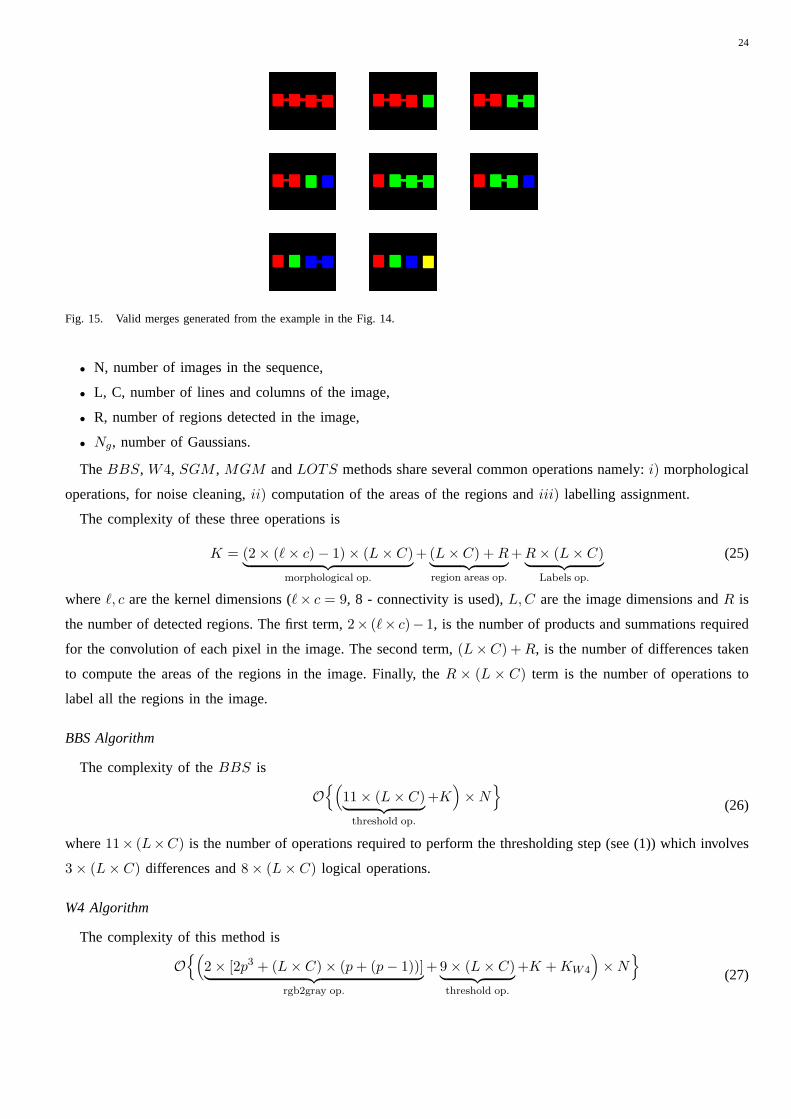
Algorithm 2 checks each sequence taking into account the relative position of the objects in the image. For
example, configurations1212,1213 are considered as invalid since object A cannot be merged with C (see Fig. 14).
Equations (24)(a) and (b) show the output of the first and the second step respectively. All the labelling sequences
considered as valid (the content of the matrixMFINAL) provides the resulting images shown in Fig. 15.
M =
1 1 1 11 1 1 21 1 2 11 1 2 21 1 2 31 2 1 11 2 1 21 2 1 31 2 2 11 2 2 21 2 2 31 2 3 11 2 3 21 2 3 31 2 3 4
(a)
MFINAL =
1 1 1 11 1 1 2
1 1 2 21 1 2 3
1 2 2 21 2 2 3
1 2 3 31 2 3 4
(b)
(24)
B. Computational Complexity
Computational complexity was also studied to judge the performance of the five algorithms. Next, we provide
comparative data on computational complexity using the “Big-O” analysis.
Let us define the following variables:
24
Fig. 15. Valid merges generated from the example in the Fig. 14.
• N, number of images in the sequence,
• L, C, number of lines and columns of the image,
• R, number of regions detected in the image,
• Ng, number of Gaussians.
TheBBS, W4, SGM , MGM andLOTS methods share several common operations namely:i) morphological
operations, for noise cleaning,ii) computation of the areas of the regions andiii) labelling assignment.
The complexity of these three operations is
K = (2× (ℓ× c)− 1)× (L× C)︸ ︷︷ ︸
morphological op.
+ (L× C) + R︸ ︷︷ ︸
region areas op.
+ R× (L× C)︸ ︷︷ ︸
Labels op.
(25)
whereℓ, c are the kernel dimensions (ℓ× c = 9, 8 - connectivity is used),L, C are the image dimensions andR is
the number of detected regions. The first term,2× (ℓ× c)− 1, is the number of products and summations required
for the convolution of each pixel in the image. The second term, (L×C) + R, is the number of differences taken
to compute the areas of the regions in the image. Finally, theR × (L × C) term is the number of operations to
label all the regions in the image.
BBS Algorithm
The complexity of theBBS is
O{(
11× (L× C)︸ ︷︷ ︸
threshold op.
+K)
×N}
(26)
where11× (L×C) is the number of operations required to perform the thresholding step (see (1)) which involves
3× (L× C) differences and8× (L× C) logical operations.
W4 Algorithm
The complexity of this method is
O{(
2× [2p3 + (L× C)× (p + (p− 1))]︸ ︷︷ ︸
rgb2gray op.
+ 9× (L× C)︸ ︷︷ ︸
threshold op.
+K + KW4
)
×N}
(27)
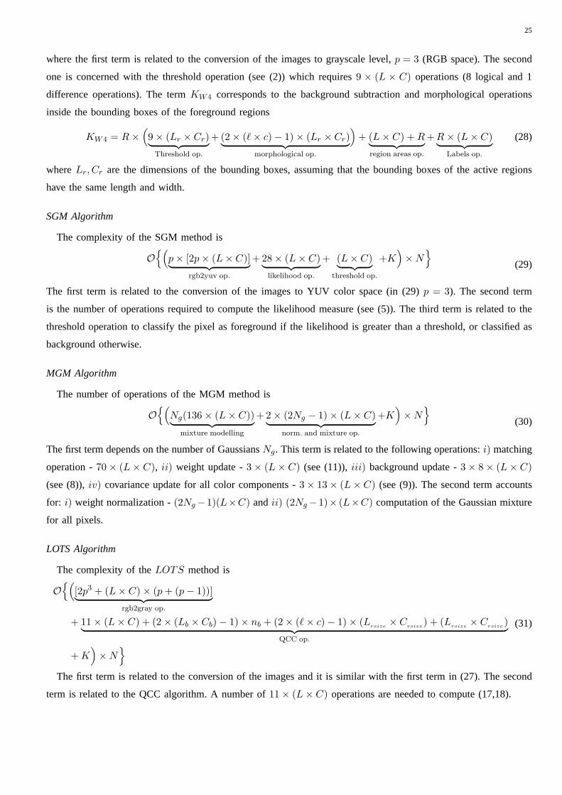
25
where the first term is related to the conversion of the images to grayscale level,p = 3 (RGB space). The second
one is concerned with the threshold operation (see (2)) which requires9 × (L × C) operations (8 logical and 1
difference operations). The termKW4 corresponds to the background subtraction and morphological operations
inside the bounding boxes of the foreground regions
KW4 = R×(
9× (Lr × Cr)︸ ︷︷ ︸
Threshold op.
+ (2× (ℓ× c)− 1)× (Lr × Cr)︸ ︷︷ ︸
morphological op.
)
+ (L× C) + R︸ ︷︷ ︸
region areas op.
+ R× (L× C)︸ ︷︷ ︸
Labels op.
(28)
whereLr, Cr are the dimensions of the bounding boxes, assuming that the bounding boxes of the active regions
have the same length and width.
SGM Algorithm
The complexity of the SGM method is
O{(
p× [2p× (L× C)]︸ ︷︷ ︸
rgb2yuv op.
+ 28× (L× C)︸ ︷︷ ︸
likelihood op.
+ (L× C)︸ ︷︷ ︸
threshold op.
+K)
×N}
(29)
The first term is related to the conversion of the images to YUV color space (in (29)p = 3). The second term
is the number of operations required to compute the likelihood measure (see (5)). The third term is related to the
threshold operation to classify the pixel as foreground if the likelihood is greater than a threshold, or classified as
background otherwise.
MGM Algorithm
The number of operations of the MGM method is
O{(
Ng(136× (L× C))︸ ︷︷ ︸
mixture modelling
+ 2× (2Ng − 1)× (L× C)︸ ︷︷ ︸
norm. and mixture op.
+K)
×N}
(30)
The first term depends on the number of GaussiansNg. This term is related to the following operations:i) matching
operation -70× (L× C), ii) weight update -3× (L× C) (see (11)),iii) background update -3× 8× (L× C)
(see (8)),iv) covariance update for all color components -3× 13× (L× C) (see (9)). The second term accounts
for: i) weight normalization -(2Ng−1)(L×C) andii) (2Ng−1)× (L×C) computation of the Gaussian mixture
for all pixels.
LOTS Algorithm
The complexity of theLOTS method is
O{(
[2p3 + (L× C)× (p + (p− 1))]︸ ︷︷ ︸
rgb2gray op.
+ 11× (L× C) + (2× (Lb × Cb)− 1)× nb + (2× (ℓ× c)− 1)× (Lrsize× C
rsize) + (L
rsize× C
rsize)
︸ ︷︷ ︸
QCC op.
+ K)
×N}
(31)
The first term is related to the conversion of the images and it issimilar with the first term in (27). The second
term is related to the QCC algorithm. A number of11× (L× C) operations are needed to compute (17,18).
26
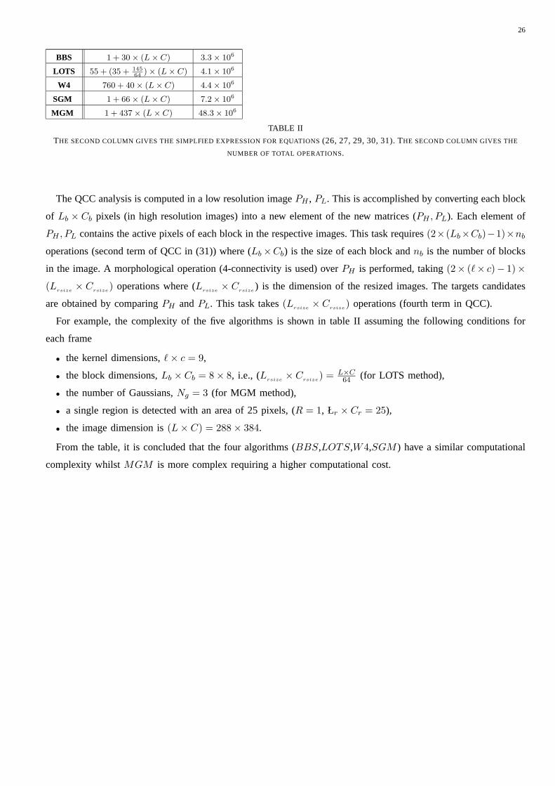
BBS 1 + 30× (L× C) 3.3× 10⁶
LOTS 55 + (35 + 145
64)× (L× C) 4.1× 10⁶
W4 760 + 40× (L× C) 4.4× 10⁶
SGM 1 + 66× (L× C) 7.2× 10⁶
MGM 1 + 437× (L× C) 48.3× 10⁶
TABLE II
THE SECOND COLUMN GIVES THE SIMPLFIED EXPRESSION FOR EQUATIONS (26, 27, 29, 30, 31). THE SECOND COLUMN GIVES THE
NUMBER OF TOTAL OPERATIONS.
The QCC analysis is computed in a low resolution imagePH , PL. This is accomplished by converting each block
of Lb × Cb pixels (in high resolution images) into a new element of the new matrices (PH , PL). Each element of
PH , PL contains the active pixels of each block in the respective images. This task requires(2×(Lb×Cb)−1)×nb
operations (second term of QCC in (31)) where (Lb×Cb) is the size of each block andnb is the number of blocks
in the image. A morphological operation (4-connectivity isused) overPH is performed, taking(2× (ℓ× c)− 1)×
(Lrsize× C
rsize) operations where (L
rsize× C
rsize) is the dimension of the resized images. The targets candidates
are obtained by comparingPH andPL. This task takes(Lrsize× C
rsize) operations (fourth term in QCC).
For example, the complexity of the five algorithms is shown intable II assuming the following conditions for
each frame
• the kernel dimensions,ℓ× c = 9,
• the block dimensions,Lb × Cb = 8× 8, i.e., (Lrsize× C
rsize) = L×C
64 (for LOTS method),
• the number of Gaussians,Ng = 3 (for MGM method),
• a single region is detected with an area of 25 pixels, (R = 1, Łr × Cr = 25),
• the image dimension is(L× C) = 288× 384.
From the table, it is concluded that the four algorithms (BBS,LOTS,W4,SGM ) have a similar computational
complexity whilstMGM is more complex requiring a higher computational cost.
27
REFERENCES
[1] C. R. Wren, A. Azarbayejani, T. Darrell, and A. P. Pentland, “Pfinder: Real-time tracking of the human body,”IEEE Trans. PatternAnal. Machine Intell., vol. 19, no. 7, pp. 780–785, July 1997.
[2] C. Stauffer, W. Eric, and L. Grimson, “Learning patterns of activity using real-time tracking,”IEEE Trans. Pattern Anal. MachineIntell., vol. 22, no. 8, pp. 747–757, August 2000.
[3] S. J. McKenna and S. Gong, “Tracking colour objects using adaptive mixture models,”Image Vision Computing, vol. 17, pp. 225–231,1999.
[4] N. Ohta, “A statistical approach to background suppression for surveillance systems,” inProceedings of IEEE Int. Conference onComputer Vision, 2001, pp. 481–486.
[5] I. Haritaoglu, D. Harwood, and L. S. Davis, “W4: Who? when? where? what? a real time system for detecting and tracking people,”
in IEEE International Conference on Automatic Face and Gesture Recognition, April 1998, pp. 222–227.[6] M. Seki, H. Fujiwara, and K. Sumi, “A robust background subtraction method for changing background,” inProceedings of IEEE
Workshop on Applications of Computer Vision, 2000, pp. 207–213.[7] D. Koller, J. Weber, T. Huang, J. Malik, G. Ogasawara, B. Rao, and S. Russel, “Towards robust automatic traffic scene analysis in
real-time,” in Proceedings of Int. Conference on Pattern Recognition, 1994, pp. 126–131.[8] R. Collins, A. Lipton, and T. Kanade, “A system for video surveillance and monitoring,” inProc. American Nuclear Society (ANS)
Eighth Int. Topical Meeting on Robotic and Remote Systems, Pittsburgh, PA, April 1999, pp. 25–29.[9] H. V. Trees,Detection, Estimation, and Modulation Theory. John Wiley and Sons, 2001.
[10] T. H. Chalidabhongse, K. Kim, D. Harwood, and L. Davis, “A perturbation method for evaluating background subtraction algorithms,”in Proc. Joint IEEE International Workshop on Visual Surveillance and Performance Evaluation of Tracking and Surveillance (VS-PETS2003), Nice, France, October 2003.
[11] X. Gao, T.E.Boult, F. Coetzee, and V. Ramesh, “Error analysisof background adaption,” inIEEE Computer Society Conference onComputer Vision and Pattern Recognition, 2000, pp. 503–510.
[12] F. Oberti, A. Teschioni, and C. S. Regazzoni, “Roc curves for performance evaluation of video sequences processing systems forsurveillance applications,” inIEEE Int. Conf. on Image Processing, vol. 2, 1999, pp. 949–953.
[13] J. Black, T. Ellis, and P. Rosin, “A novel method for video trackingperformance evaluation,” inJoint IEEE Int. Workshop on VisualSurveillance and Performance Evaluation of Tracking and Surveillance (VS-PETS), Nice, France, 2003, pp. 125–132.
[14] P. Correia and F. Pereira, “Objective evaluation of relative segmentation quality,” inInt. Conference on Image Processing, 2000, pp.308–311.
[15] C. E. Erdem, B. Sankur, and A. M.Tekalp, “Performance measures for video object segmentation and tracking,”IEEE Trans. ImageProcessing, vol. 13, no. 7, pp. 937–951, 2004.
[16] V. Y. Mariano, J. Min, J.-H. Park, R. Kasturi, D. Mihalcik, H. Li, D. Doermann, and T. Drayer, “Performance evaluation of objectdetection algorithms,” inProceedings of 16th Int. Conf. on Pattern Recognition (ICPR02), vol. 3, 2002, pp. 965–969.
[17] I. Haritaoglu, D. Harwood, and L. S. Davis, “W4: real-time surveillance of people and their activities,”IEEE Trans. Pattern Anal.
Machine Intell., vol. 22, no. 8, pp. 809–830, August 2000.[18] T. Boult, R. Micheals, X. Gao, and M. Eckmann, “Into the woods: Visual surveillance of non-cooperative camouflaged targets in
complex outdoor settings,” inProceedings of the IEEE, October 2001, pp. 1382–1402.[19] R. C. Gonzalez and R. E. Woods,Digital Image Processing. Prentice Hall, 2002.[20] R. Cucchiara, C. Grana, M. Piccardi, and A. Prati, “Detecting moving objects, ghosts and shadows in video streams,”IEEE Trans.
Pattern Anal. Machine Intell., vol. 25, no. 10, pp. 1337–1342, 2003.[21] Y.-F. Ma and H.-J. Zhang, “Detecting motion object by spatio-temporal entropy,” inIEEE Int. Conf. on Multimedia and Expo, Tokyo,
Japan, August 2001.[22] R. Souvenir, J. Wright, and R. Pless, “Spatio-temporal detection and isolation: Results on the PETS2005 datasets,” inProceedings of
the IEEE Workshop on Performance Evaluation in Tracking and Surveillance, 2005.[23] H. Sun, T. Feng, and T. Tan, “Spatio-temporal segmentation forvideo surveillance,” inIEEE Int. Conf. on Pattern Recognition, vol. 1,
Barcelona, Spain, September, pp. 843–846.[24] A. Monnet, A. Mittal, N. Paragios, and V. Ramesh, “Background modeling and subtraction of dynamic scenes,” inProceedings of the
ninth IEEE Int. Conf. on Computer Vision, 2003, pp. 1305–1312.[25] J. Zhong and S. Sclaroff., “Segmenting foreground objects from a dynamic, textured background via a robust kalman filter,” in
Proceedings of the ninth IEEE Int. Conf. on Computer Vision, 2003, pp. 44–50.[26] N. T. Siebel and S. J. Maybank, “Real-time tracking of pedestrians and vehicles,” inProc. of IEEE workshop on Performance Evaluation
of tracking and surveillance, 2001.[27] R. Cucchiara, C. Grana, and A. Prati, “Detecting moving objects and their shadows: an evaluation with the PETS2002 dataset,” in
Proceedings of Third IEEE International Workshop on Performance Evaluation of Tracking and Surveillance (PETS 2002) in conj. withECCV 2002, Pittsburgh, PA, May 2002, pp. 18–25.
[28] Collins, Lipton, Kanade, Fujiyoshi, Duggins, Tsin, Tolliver, Enomoto, and Hasegawa, “A system for video surveillance and monitoring:Vsam final report,” Robotics Institute, Carnegie Mellon University, Tech. Rep. Technical report CMU-RI-TR-00-12, May 2000.
[29] T. Boult, R. Micheals, X. Gao, W. Y. P. Lewis, C. Power, and A. Erkan, “Frame-rate omnidirectional surveillance and tracking ofcamouflaged and occluded targets,” inSecond IEEE International Workshop on Visual Surveillance, 1999, pp. 48–55.