Embed Size (px)
Citation preview
1
Particular solutions for some engineering problems
Chia-Cheng Tasi 蔡加正
Department of Information Technology Toko University, Chia-Yi County, Taiwan
2008 NTOU
2
Motivation
Method of Particular Solutions (MPS)
Particular solutions of polyharmonic spline
Numerical example I
Particular solutions of Chebyshev polynomials
Numerical example II
Conclusions
Overview
3
Motivation
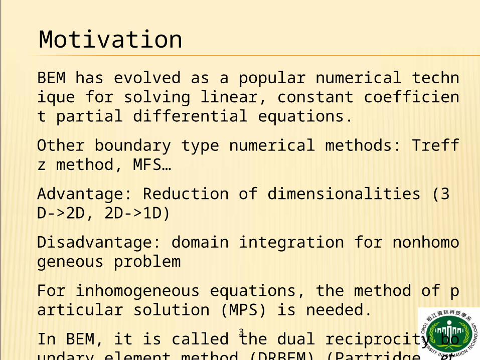
BEM has evolved as a popular numerical technique for solving linear, constant coefficient partial differential equations.
Other boundary type numerical methods: Treffz method, MFS…
Advantage: Reduction of dimensionalities (3D->2D, 2D->1D)
Disadvantage: domain integration for nonhomogeneous problem
For inhomogeneous equations, the method of particular solution (MPS) is needed.
In BEM, it is called the dual reciprocity boundary element method (DRBEM) (Partridge, et al., 1992).
4
Motivation and Literature review
5
Motivation
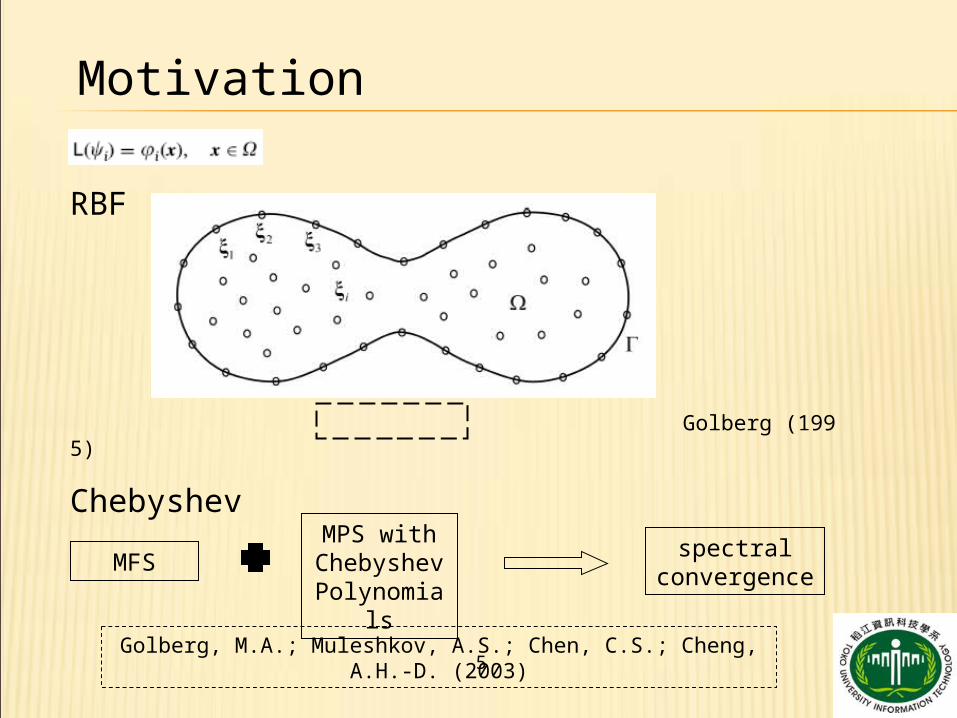
RBF
Golberg (1995)
Chebyshev
MFSMPS with
Chebyshev Polynomial
s
spectral convergence
Golberg, M.A.; Muleshkov, A.S.; Chen, C.S.; Cheng, A.H.-D. (2003)
6
Motivation
1 21 2( ) ( ) ( )
L
7
Motivation
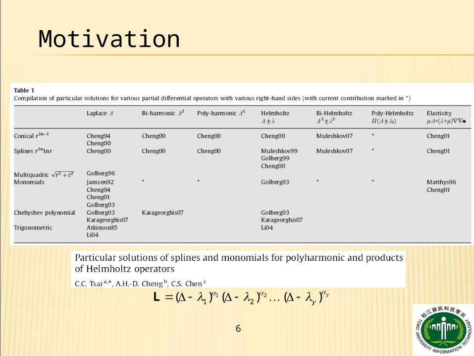
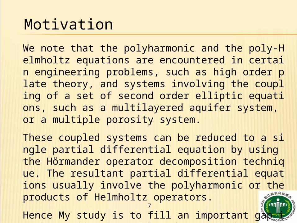
We note that the polyharmonic and the poly-Helmholtz equations are encountered in certain engineering problems, such as high order plate theory, and systems involving the coupling of a set of second order elliptic equations, such as a multilayered aquifer system, or a multiple porosity system.
These coupled systems can be reduced to a single partial differential equation by using the Hörmander operator decomposition technique. The resultant partial differential equations usually involve the polyharmonic or the products of Helmholtz operators.
Hence My study is to fill an important gap in the application of boundary methods to these engineering problems.
8
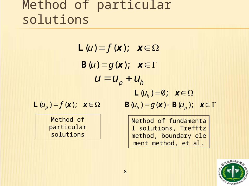
Method of particular solutions
( ) ( );u f L x x
( ) ( );u g B x x
p hu u u
( ) ( );pu f L x x
( ) 0;hu L x
( ) ( ) ( );h pu g u B Bx x
Method of particular solutions
Method of fundamental solutions, Trefftz method, boundary element metho
d, et al.
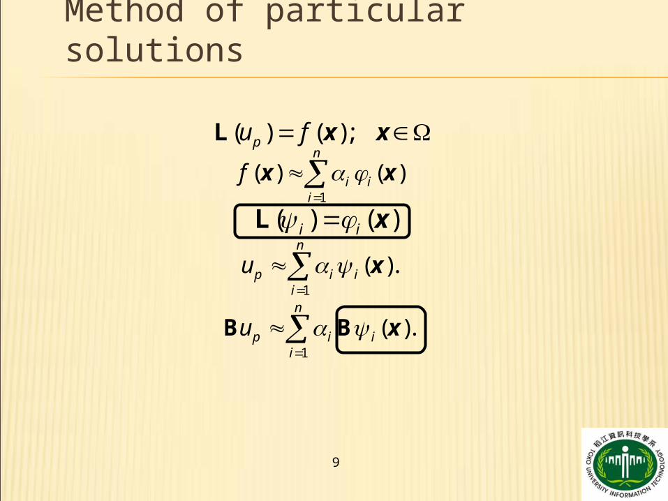
9
( ) ( );pu f L x x
1
( ) ( )n
i ii
f
x x
( ) ( )i i L x
1
( ).n
p i ii
u
x
1
( ).n
p i ii
u
B B x
Method of particular solutions
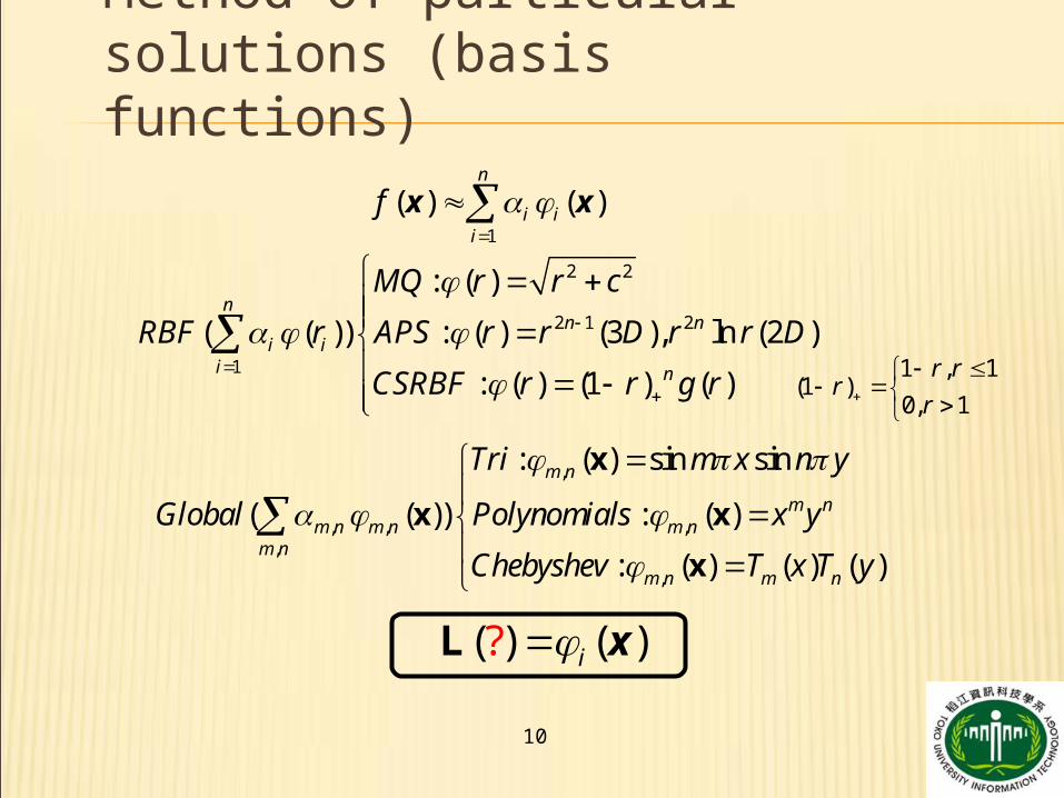
10
1
( ) ( )n
i ii
f
x x
2 2
2 1 2
1
: ( )
( ( )) : ( ) (3 ), ln (2 )
: ( ) (1 ) ( )
nn n
i ii n
MQ r r c
RBF r APS r r D r r D
CSRBF r r g r
,
, , ,,
,
: ( ) sin sin
( ( )) : ( )
: ( ) ( ) ( )
m n
m nm n m n m n
m n
m n m n
Tri m x n y
Global Polynomials x y
Chebyshev T x T y
x
x x
x
1 , 1(1 )
0, 1
r rr
r
( (?) )iL x
Method of particular solutions (basis functions)
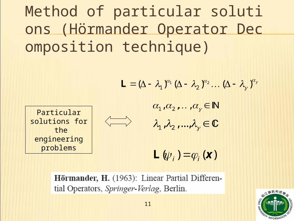
11
1 21 2( ) ( ) ( )
L
1 2, , ,
1 2, ,...,
( ) ( )i i L x
Particular solutions for
the engineering problems
Method of particular solutions (Hörmander Operator Decomposition technique)
12
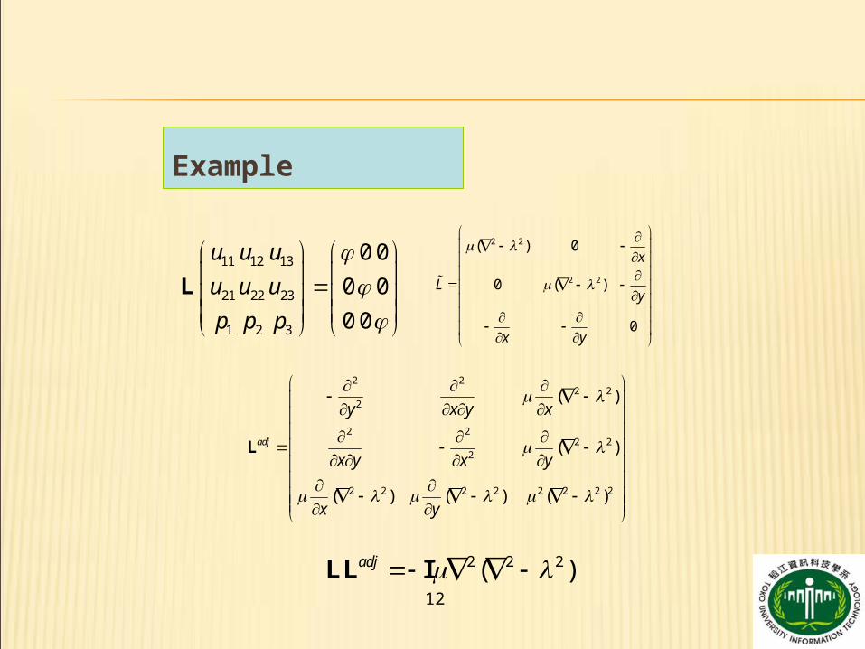
Example
11 12 13
21 22 23
1 2 3
0 0
0 0
0 0
u u u
u u u
p p p
L
2 2
2 2
( ) 0
0 ( )
0
x
Ly
x y
2 22 2
2
2 22 2
2
2 2 2 2 2 2 2 2
( )
( )
( ) ( ) ( )
adj
y x y x
x y x y
x y
L
2 2 2( )adj LL I
13
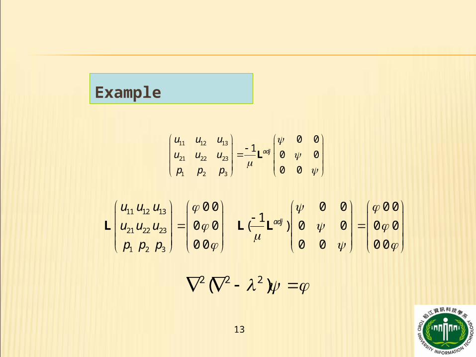
Example
11 12 13
21 22 23
1 2 3
0 01
0 0
0 0
adj
u u u
u u u
p p p
L
0 0 0 01
( ) 0 0 0 0
0 0 0 0
adj
L L11 12 13
21 22 23
1 2 3
0 0
0 0
0 0
u u u
u u u
p p p
L
2 2 2( )

14
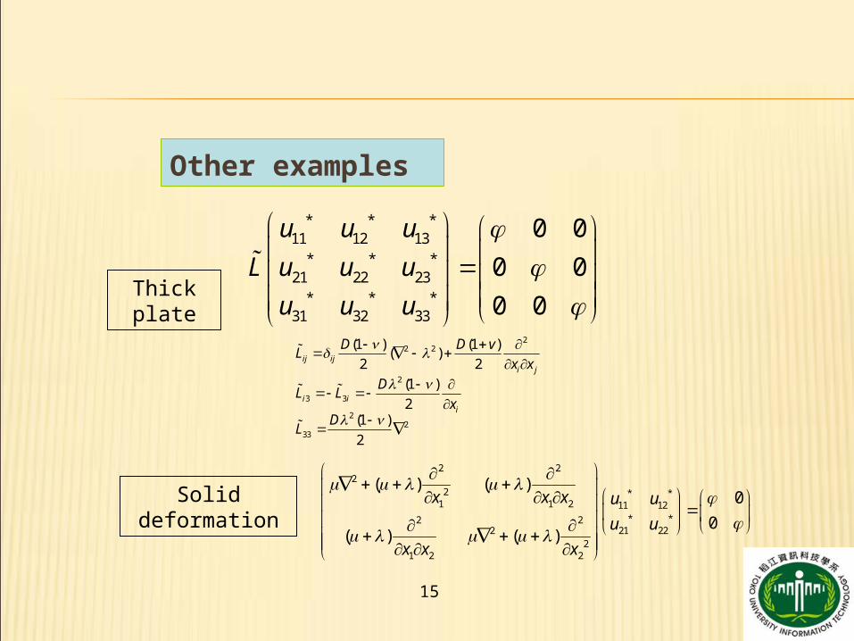
Other examples
2
11 12 132
21 22 23
1 2 3
00 0
0 0 0
0 0
0
x u u u
u u uy
p p p
x y
2
1 * * *11 12 13
2 * * *21 22 23
2 * * *2 1 2 3
* * *1 2 3
1 2
0 0
0 0 000 0 0 00
0 0 000 0 0
0 0 0 000 0
T
xu u u
u u ux
T T Tk
p p p
x x
Stokes flow
Thermal Stokes flow
15
Other examples
* * *11 12 13
* * *21 22 23
* * *31 32 33
0 0
0 0
0 0
u u u
L u u u
u u u
22 2(1 ) (1 )
( )2 2ij ij
i j
D D vL
x x
2
3 3
(1 )
2i ii
DL L
x
22
33
(1 )
2
DL
Thick plate
2 22
2 * *1 1 2 11 12
* *2 22 21 22
21 2 2
( ) ( )0
0( ) ( )
x x x u u
u u
x x x
Solid deformation
16
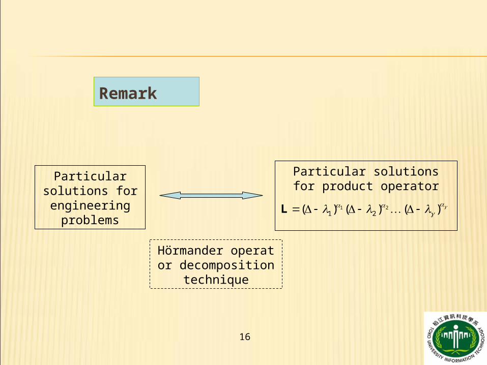
Remark
Particular solutions for engineering
problems
Particular solutions for product operator
1 21 2( ) ( ) ( )
L
Hörmander operator decomposition techn
ique
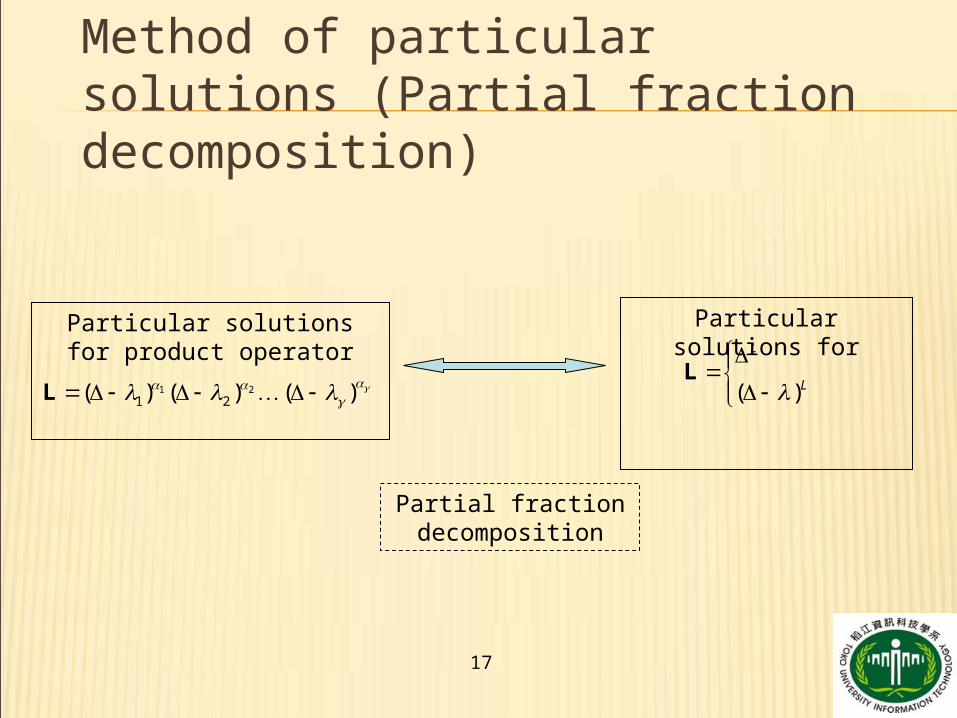
17
Particular solutions for
( )
L
L
L
Partial fraction decomposition
Particular solutions for product operator
1 21 2( ) ( ) ( )
L
Method of particular solutions (Partial fraction decomposition)
18
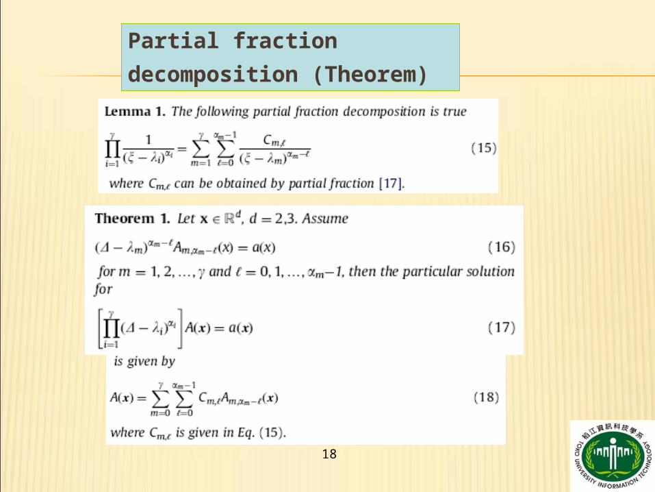
Partial fraction
decomposition (Theorem)
19
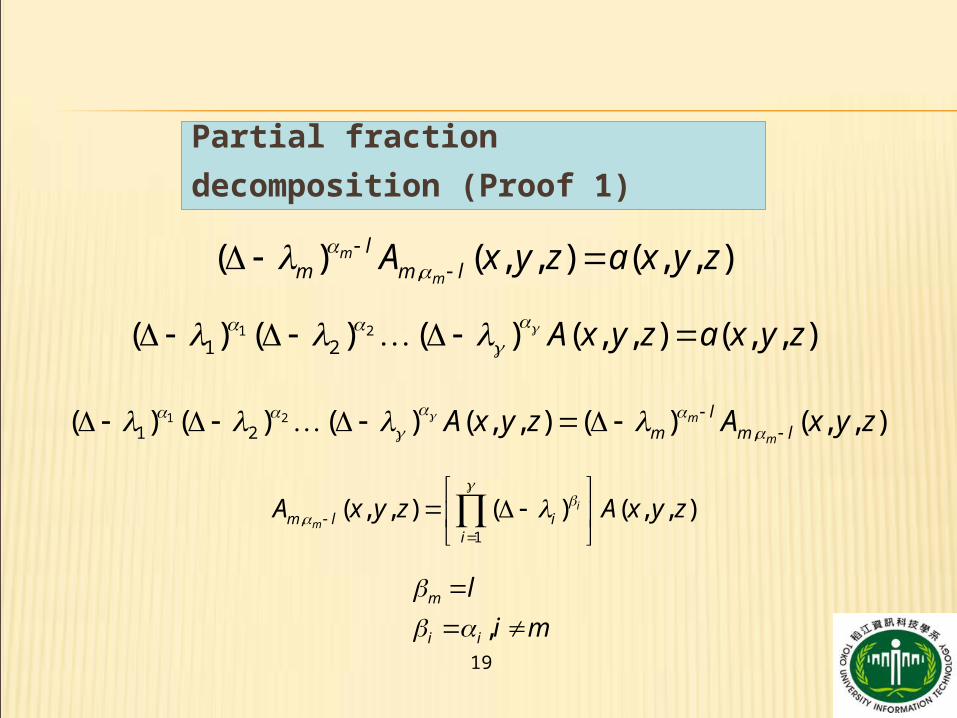
Partial fraction decomposition
(Proof 1)
,( ) ( , , ) ( , , )m
m
lm m lA x y z a x y z
1 21 2( ) ( ) ( ) ( , , ) ( , , )A x y z a x y z
1 21 2 ,( ) ( ) ( ) ( , , ) ( ) ( , , )m
m
lm m lA x y z A x y z
,1
( , , ) ( ) ( , , )i
mm l ii
A x y z A x y z
,m
i i
l
i m
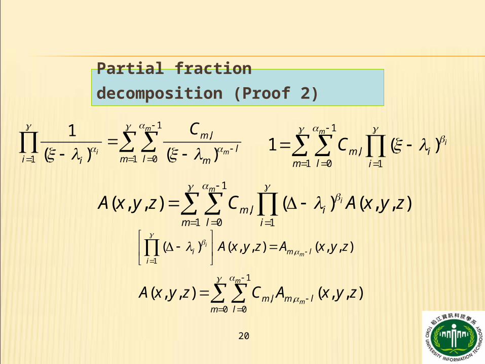
20
Partial fraction decomposition
(Proof 2)
1
,1 0 1
1 ( )m
im l i
m l i
C
1
,1 0 1
( , , ) ( ) ( , , )m
im l i
m l i
A x y z C A x y z
,
1
( ) ( , , ) ( , , )i
mi m li
A x y z A x y z
1
, ,0 0
( , , ) ( , , )m
mm l m lm l
A x y z C A x y z
1,
1 01
1
( ) ( )
m
i m
m ll
m li i m
C
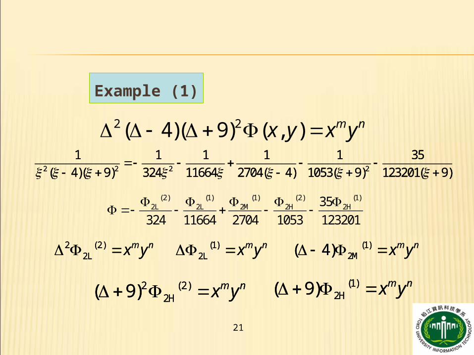
21
Example
(1)
2 2( 4)( 9) ( , ) m nx y x y
2 2 2 2
1 1 1 1 1 35
( 4)( 9) 324 11664 2704( 4) 1053( 9) 123201( 9)
(2) (1) (1) (2) (1)2L 2L 2M 2H 2H35
324 11664 2704 1053 123201
2 (2)2L
m nx y (1)2L
m nx y (1)2M( 4) m nx y
2 (2)2H( 9) m nx y (1)
2H( 9) m nx y
2 2 2 2
1 1 1 1 1 35
( 4)( 9) 324 11664 2704( 4) 1053( 9) 123201( 9)
2 (2)2L
m nx y (1)2L
m nx y (1)2M( 4) m nx y
2 (2)2H( 9) m nx y (1)
2H( 9) m nx y
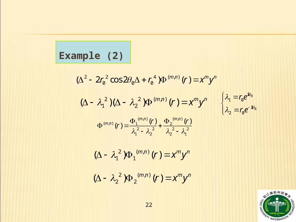
22
Example (2)
2 2 4 ( , )0 0 0( 2 cos 2 ) ( )m n m nr r r x y
2 2 ( , )1 2( )( ) ( )m n m nr x y
0
0
1 0
2 0
r e
r e
i
i
( , ) ( , )( , ) 1 2
2 2 2 21 2 2 1
( ) ( )( )
m n m nm n r r
r
2 ( , )1 1( ) ( )m n m nr x y
2 ( , )2 2( ) ( )m n m nr x y
23
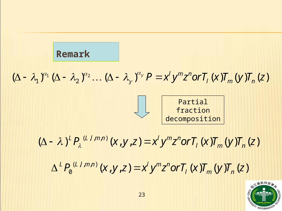
Remark
( , , , )( ) ( , , ) ( ) ( ) ( )L L l m n l m nl m nP x y z x y z orT x T y T z
( , , , )0 ( , , ) ( ) ( ) ( )L L l m n l m n
l m nP x y z x y z orT x T y T z
1 21 2( ) ( ) ( ) ( ) ( ) ( )l m n
l m nP x y z orT x T y T z
Partial fraction decomposition
24
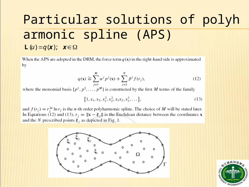
Particular solutions of polyharmonic spline (APS)
( ) ( );u q L x x
25
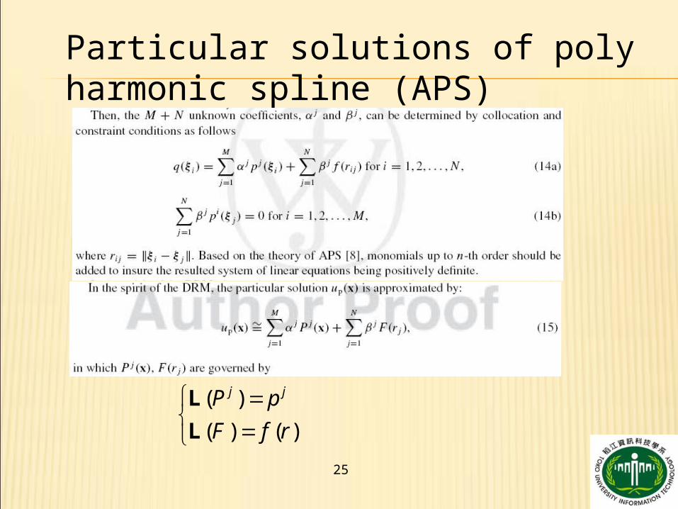
Particular solutions of polyharmonic spline (APS)
( )
( ) ( )
j jP p
F f r
L
L
26
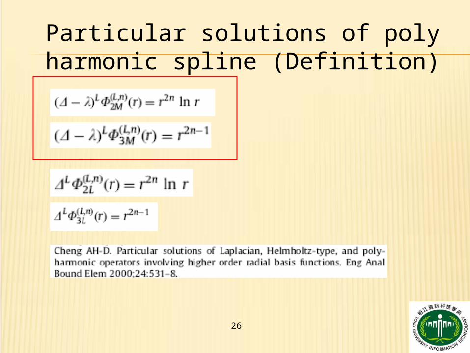
Particular solutions of polyharmonic spline (Definition)
27
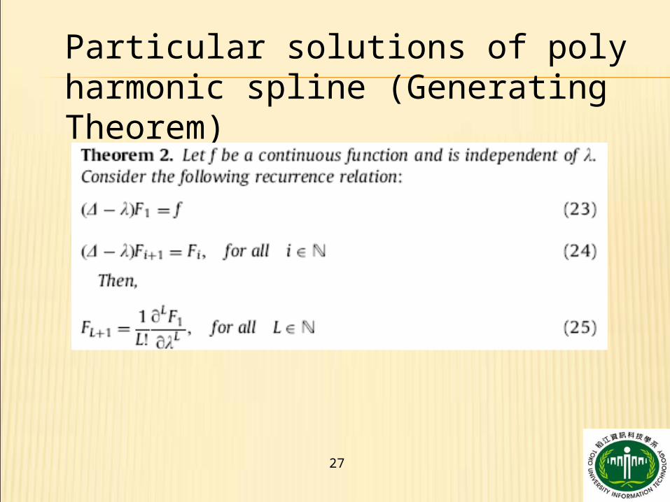
Particular solutions of polyharmonic spline (Generating Theorem)
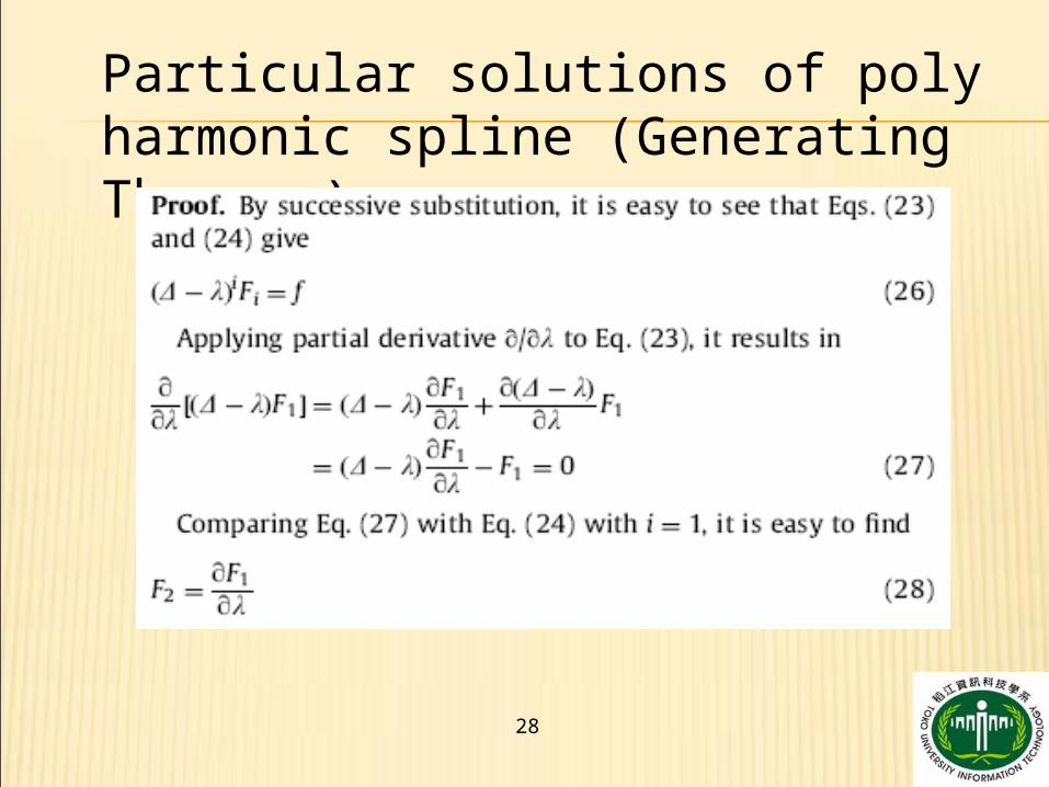
28
Particular solutions of polyharmonic spline (Generating Theorem)
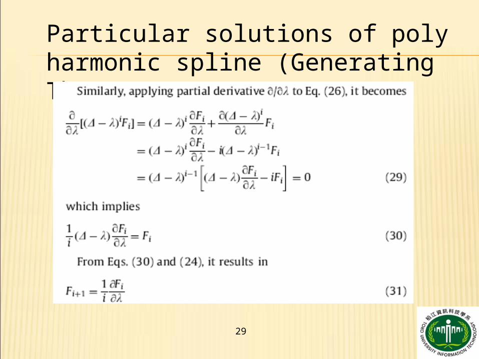
29
Particular solutions of polyharmonic spline (Generating Theorem)

30
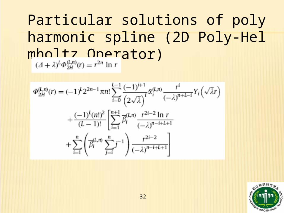
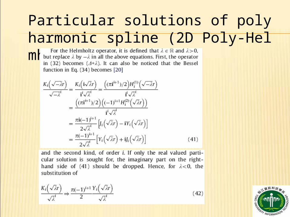
Particular solutions of polyharmonic spline (2D Poly-Helmholtz Operator)
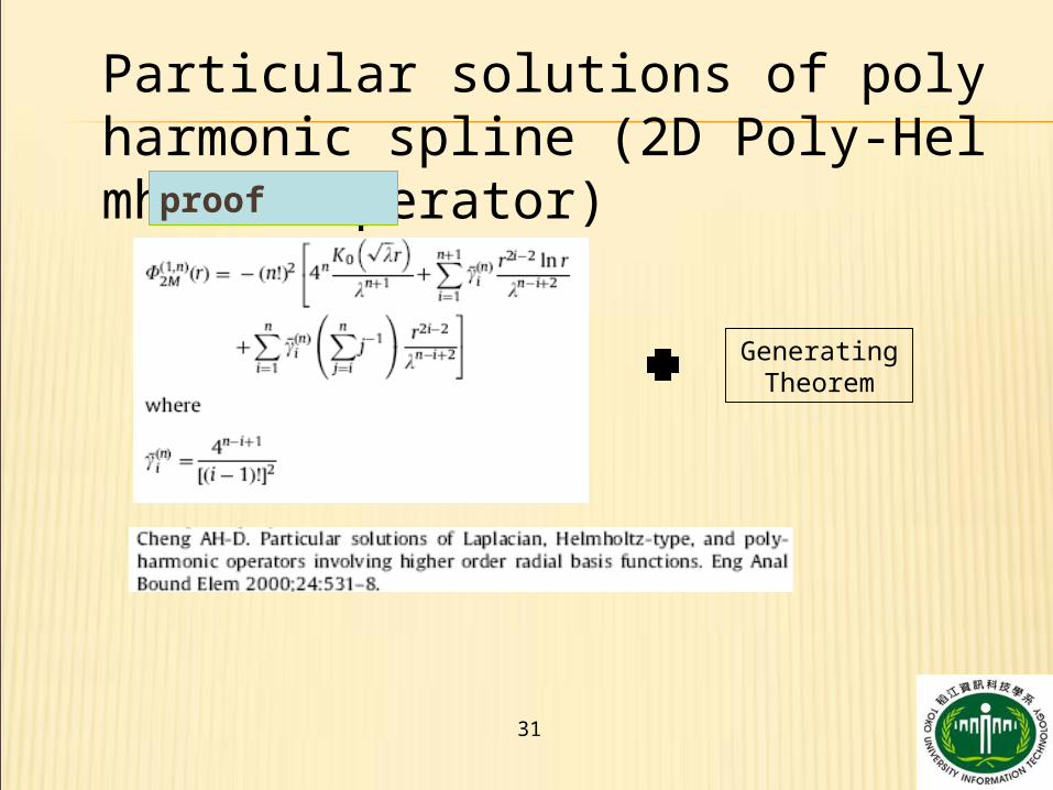
31
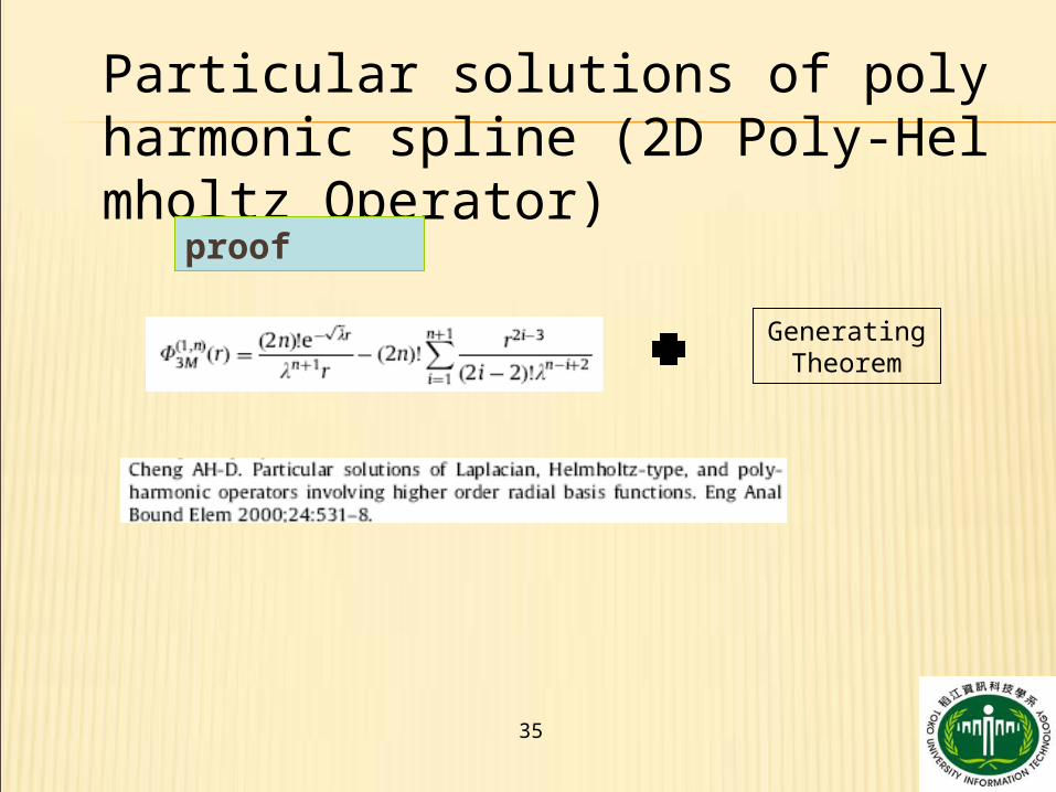
Particular solutions of polyharmonic spline (2D Poly-Helmholtz Operator)
Generating Theorem
proof
32
Particular solutions of polyharmonic spline (2D Poly-Helmholtz Operator)
33
Particular solutions of polyharmonic spline (2D Poly-Helmholtz Operator)
34
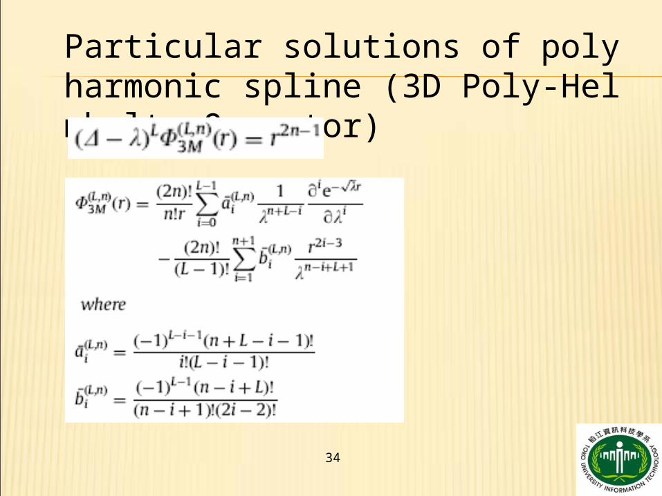
Particular solutions of polyharmonic spline (3D Poly-Helmholtz Operator)
35
Particular solutions of polyharmonic spline (2D Poly-Helmholtz Operator)
Generating Theorem
proof
36
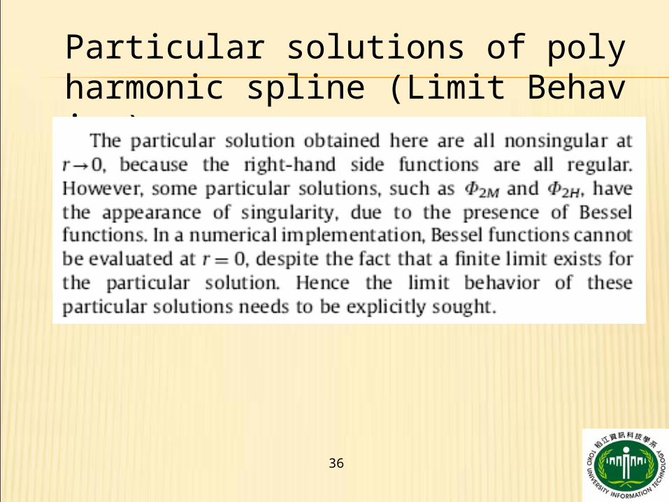
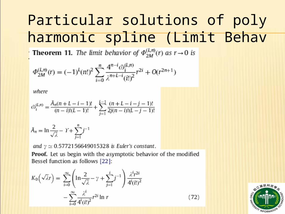
Particular solutions of polyharmonic spline (Limit Behavior)
37
Particular solutions of polyharmonic spline (Limit Behavior)
38
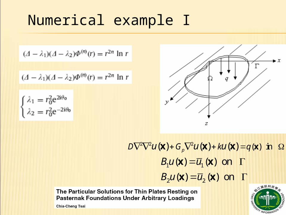
2 2 2 ( ) in ( ) ( ) ( )pD G k qu u u xx x x
Numerical example I
1 1
2 2
( ) ( ) on
( ) ( ) on
B u u
B u u
x x
x x
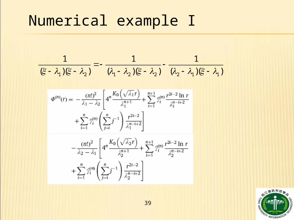
39
Numerical example I
1 2 1 2 2 2 1 1
1 1 1
( )( ) ( )( ) ( )( )
40
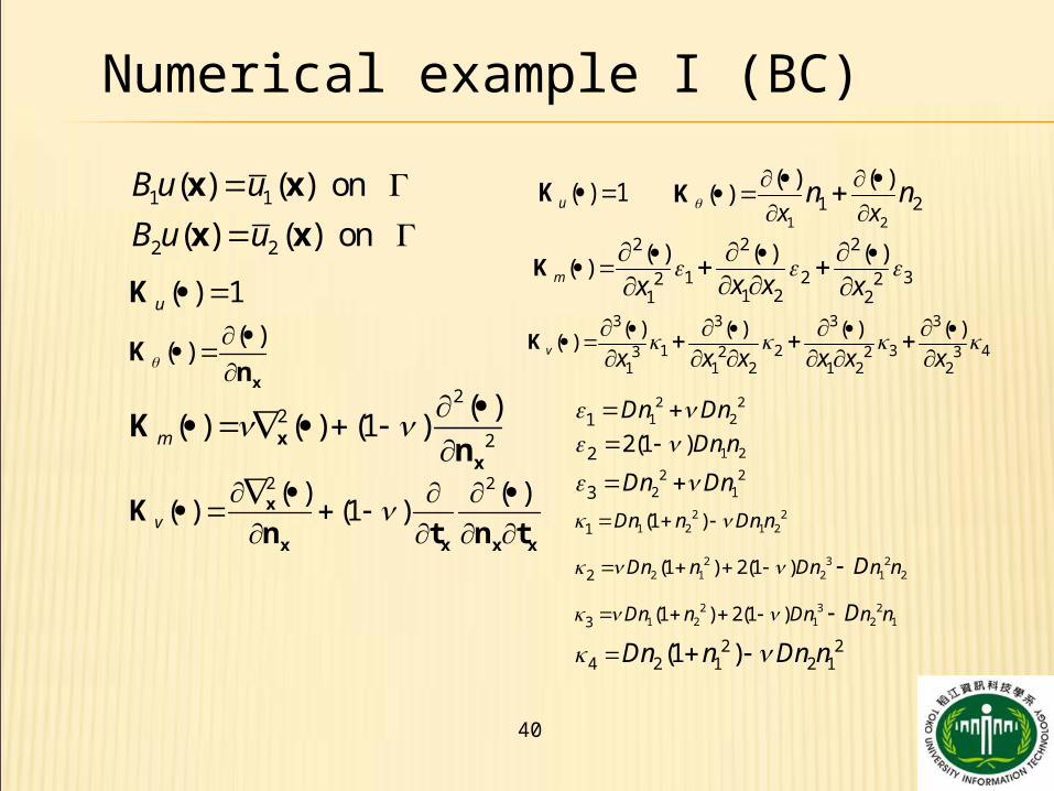
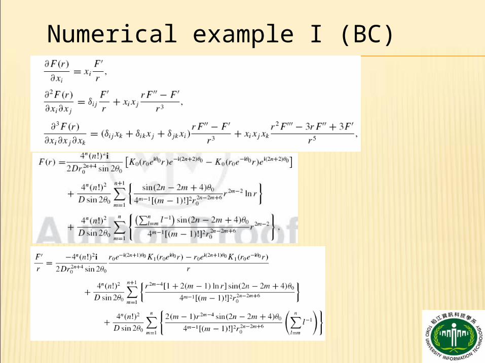
Numerical example I (BC)
( ) 1u K
1 1
2 2
( ) ( ) on
( ) ( ) on
B u u
B u u
x x
x x
( )( )
x
Kn
22
2
( )( ) ( ) (1 )m
xx
Kn
2 2( ) ( )( ) (1 )v
x
x x x x
Kn t n t
( ) 1u K1 2
1 2( ) ( )
( )x x
n n
K
2 2 2
1 2 32 21 21 2
( ) ( ) ( )( )m x xx x
K
3 3 3 3
1 2 3 43 2 2 31 1 2 1 2 2
( ) ( ) ( ) ( )( )v x x x x x x
K
2 21 21 Dn Dn
1 22 2(1 )Dn n 2 2
2 13 Dn Dn 2 2
1 2 1 21 (1 )Dn n Dn n
2 3 22 1 2 1 22 (1 ) 2(1 )Dn n Dn n nD
2 3 21 2 1 2 13 (1 ) 2(1 )Dn n Dn n nD
2 24 2 1 2 1(1 )Dn n Dn n
41
Numerical example I (BC)
42
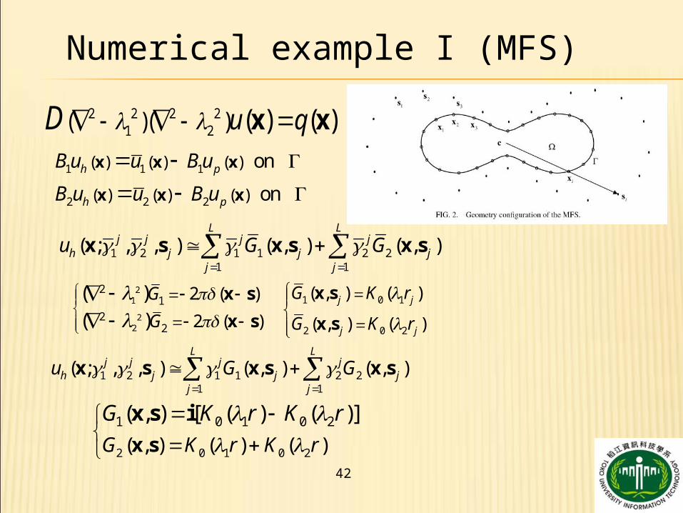
Numerical example I (MFS)
1 1 1
2 2 2
( ) ( ) ( )
( ) ( ) ( )
on
on
h p
h p
B u u B u
B u u B u
x x x
x x x
1 2 1 1 2 21 1
( ; , , ) ( , ) ( , )L L
j j j jh j j j
j j
u G G
x s x s x s
1 0 1
2 0 2
( , ) ( )
( , ) ( )
j j
j j
G K r
G K r
x s
x s
21
22
21
22
2 ( )
2 ( )
( )( )
G
G
x s
x s
1 2 1 1 2 21 1
( ; , , ) ( , ) ( , )L L
j j j jh j j j
j j
u G G
x s x s x s
2 0 1 0 2
1 0 1 0 2
( , ) ( ) ( )
( , ) [ ( ) ( )]
G K r K r
G K r K r
x s
x s i
2 2 2 21 2( )( ) ( ) ( )u qD x x
43
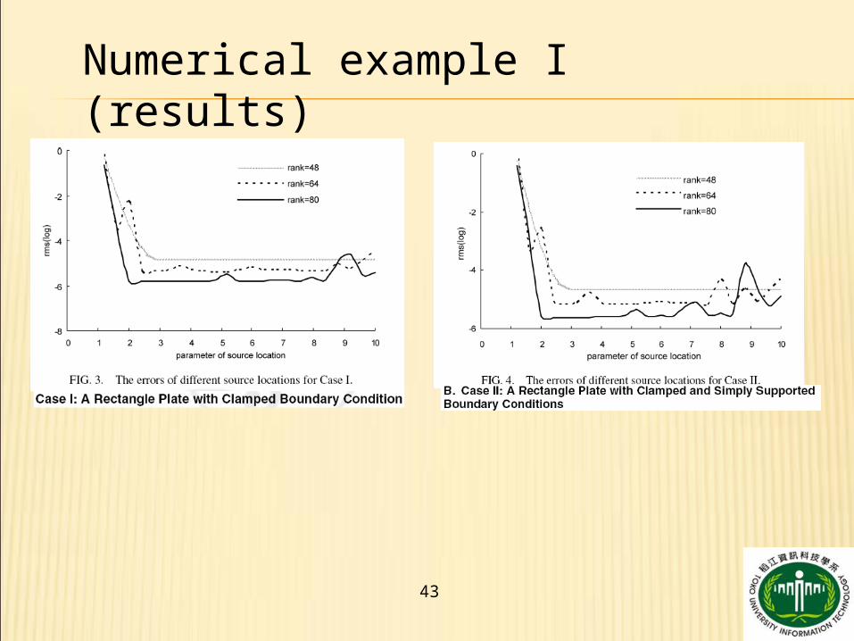
Numerical example I (results)
44
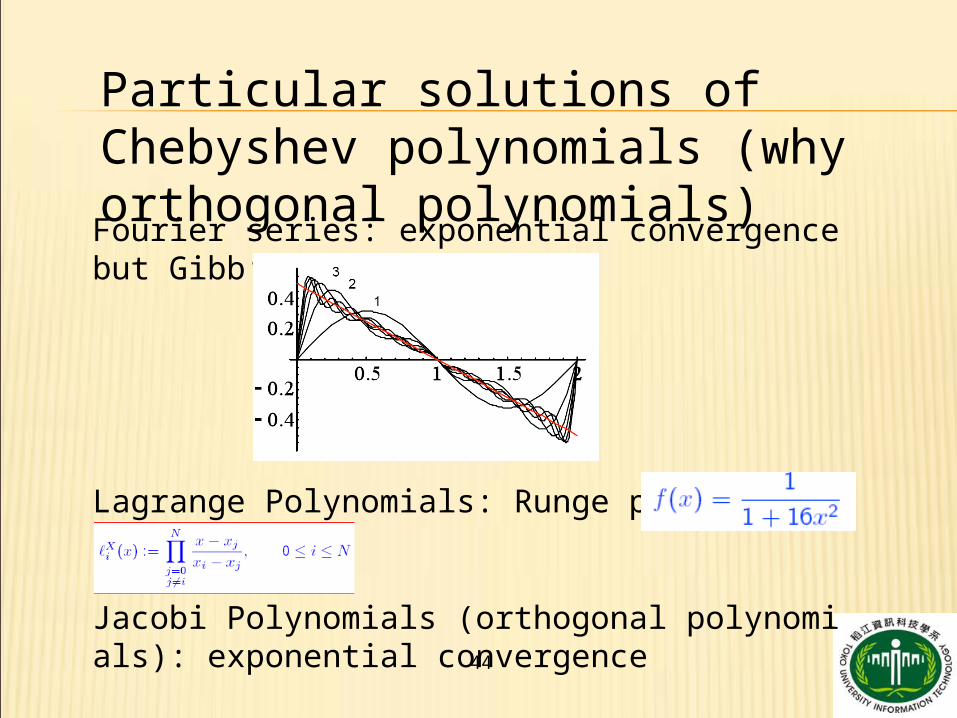
Particular solutions of Chebyshev polynomials (why orthogonal polynomials)Fourier series: exponential convergence but Gibb’s phenomena
Lagrange Polynomials: Runge phenomena
Jacobi Polynomials (orthogonal polynomials): exponential convergence
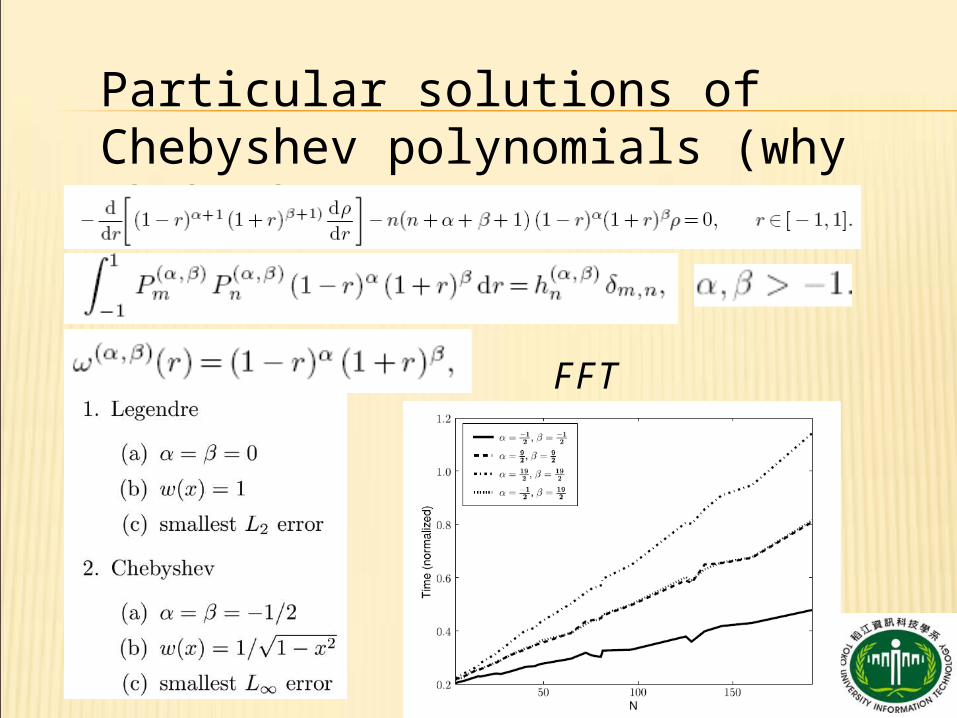
45
Particular solutions of Chebyshev polynomials (why Chebyshev)
FFT
46
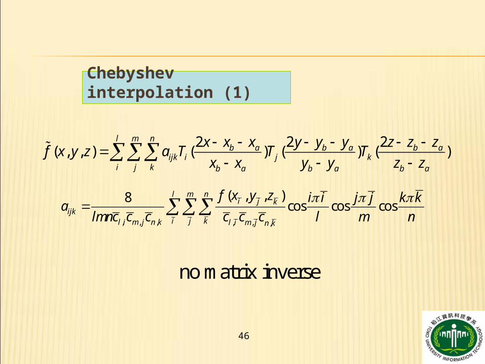
Chebyshev interpolation (1)
2 2 2( , , ) ( ) ( ) ( )
l m nb a b a b a
ijk i j ki j k b a b a b a
x x x y y y z z zf x y z a T T T
x x y y z z
, , , , , ,
( , , )8cos cos cos
l m ni j k
ijki j kl i m j n k l i m j n k
f x y z i i j j k ka
lmnc c c c c c l m n
no matrix inverse
47
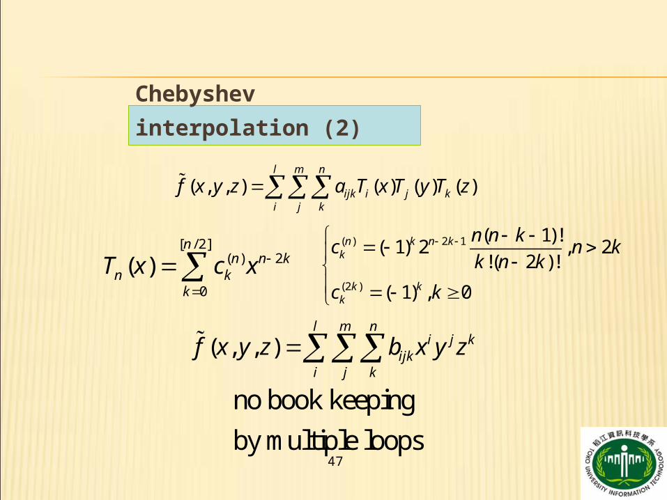
Chebyshev
interpolation (2)
( , , ) ( ) ( ) ( )l m n
ijk i j ki j k
f x y z a T x T y T z
[ / 2]( ) 2
0
( )n
n n kn k
k
T x c x
( ) 2 1
(2 )
( 1)!( 1) 2 , 2
!( 2 )!
( 1) , 0
n k n kk
k kk
n n kc n k
k n k
c k
( , , )l m n
i j kijk
i j k
f x y z b x y z
no book keeping
by multiple loops
48
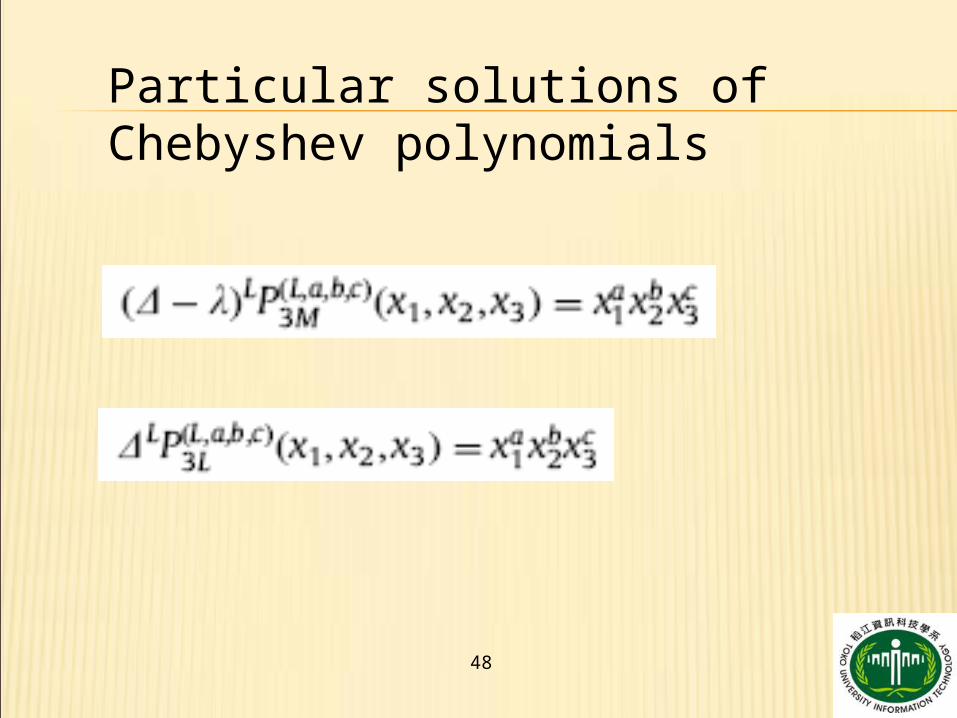
Particular solutions of Chebyshev polynomials
49
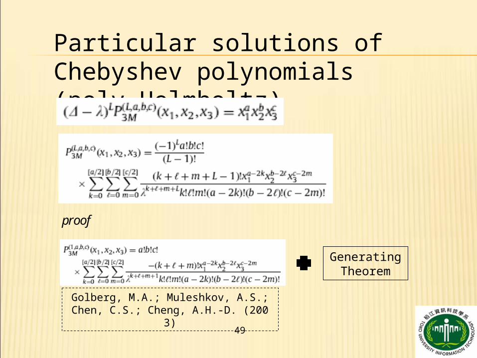
Particular solutions of Chebyshev polynomials (poly-Helmholtz)
proof
Generating Theorem
Golberg, M.A.; Muleshkov, A.S.; Chen, C.S.; Cheng, A.H.-D. (2003)
50
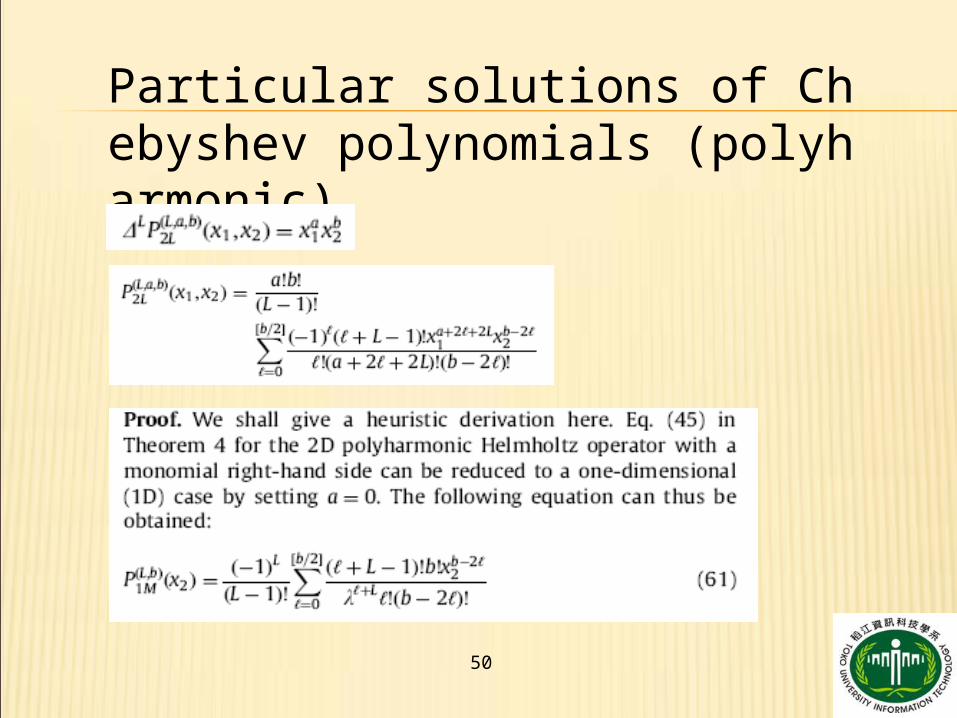
Particular solutions of Chebyshev polynomials (polyharmonic)
51
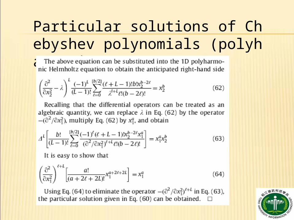
Particular solutions of Chebyshev polynomials (polyharmonic)
52
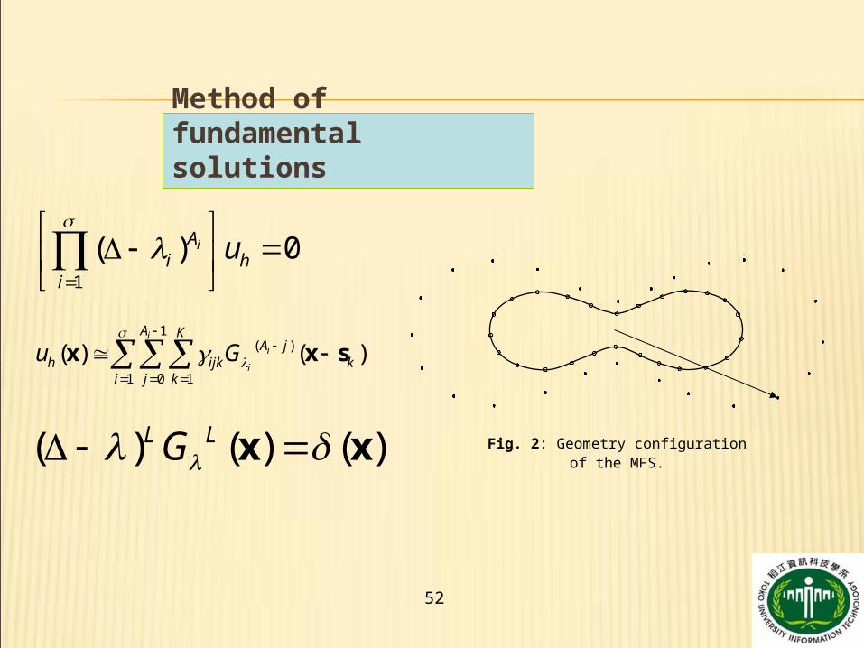
Method of fundamental solutions
1
( ) 0iAi h
i
u
1( )
1 0 1
( ) ( )i
i
i
A KA j
h ijk ki j k
u G
x x s
( ) ( ) ( )L LG x x Fig. 2: Geometry configuration of the MFS.
53
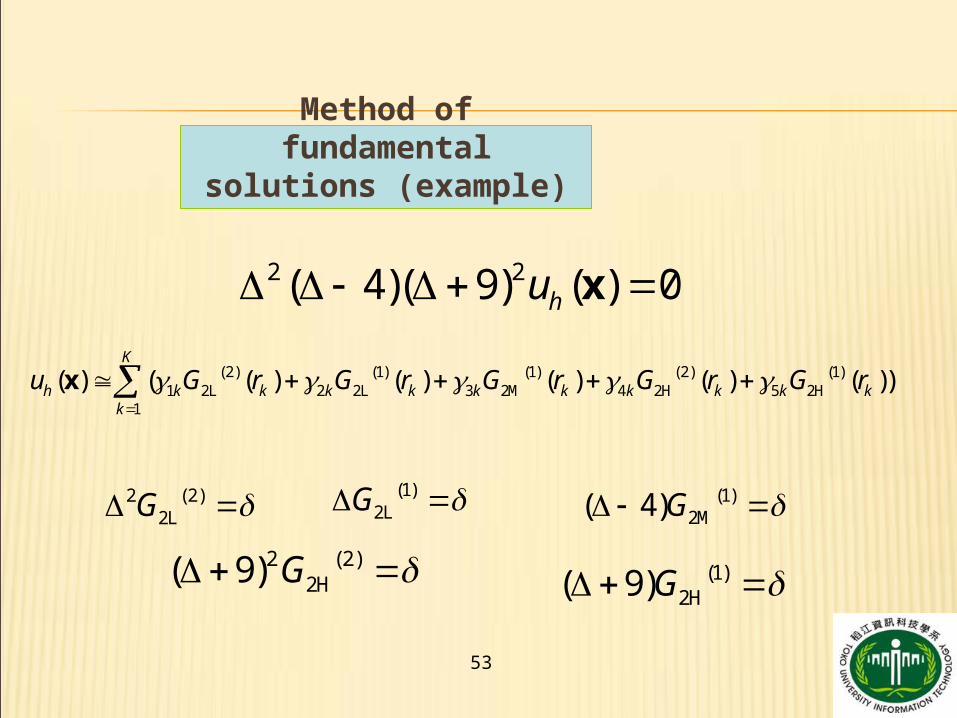
2 2( 4)( 9) ( ) 0hu x
2 (2)2LG
(1)2LG (1)
2M( 4)G
2 (2)2H( 9) G (1)
2H( 9)G
(2) (1) (1) (2) (1)1 2L 2 2L 3 2M 4 2H 5 2H
1
( ) ( ( ) ( ) ( ) ( ) ( ))K
h k k k k k k k k k kk
u G r G r G r G r G r
x
Method of fundamental
solutions (example)
54
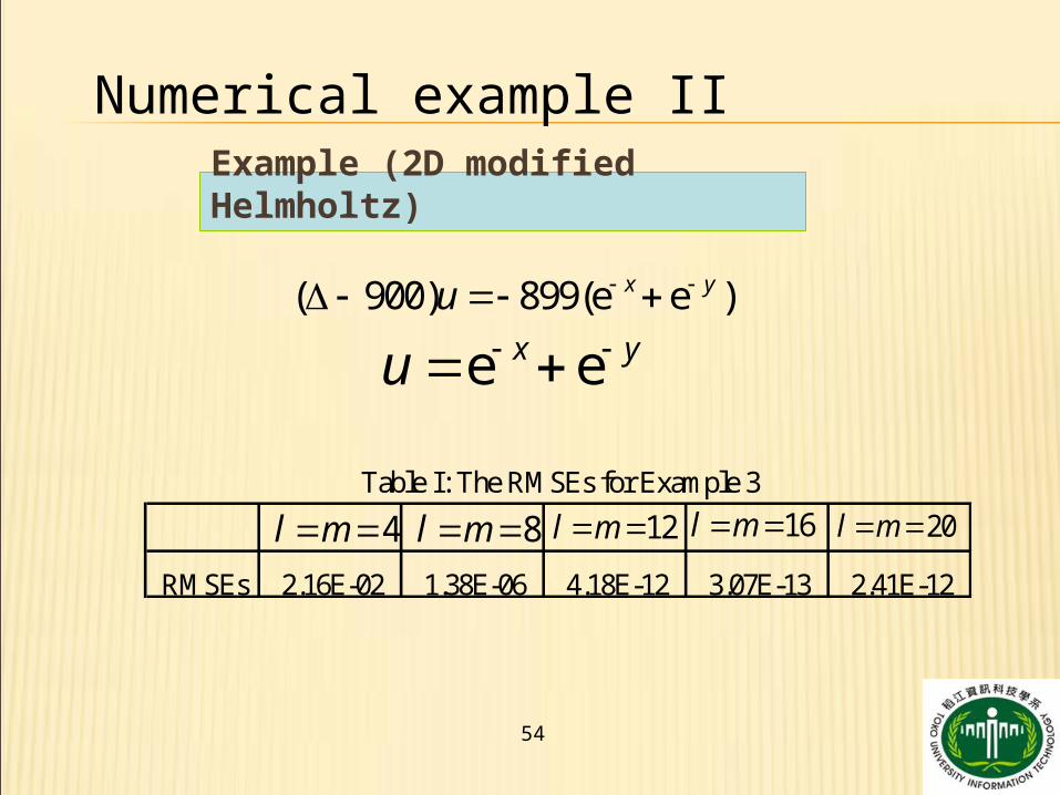
Example (2D modified Helmholtz)
( 900) 899(e e )x yu
e ex yu
RMSEs 2.16E-02 1.38E-06 4.18E-12 3.07E-13 2.41E-12
Table I: The RMSEs for Example 3
4l m 8l m 12l m 16l m 20l m
Numerical example II
55
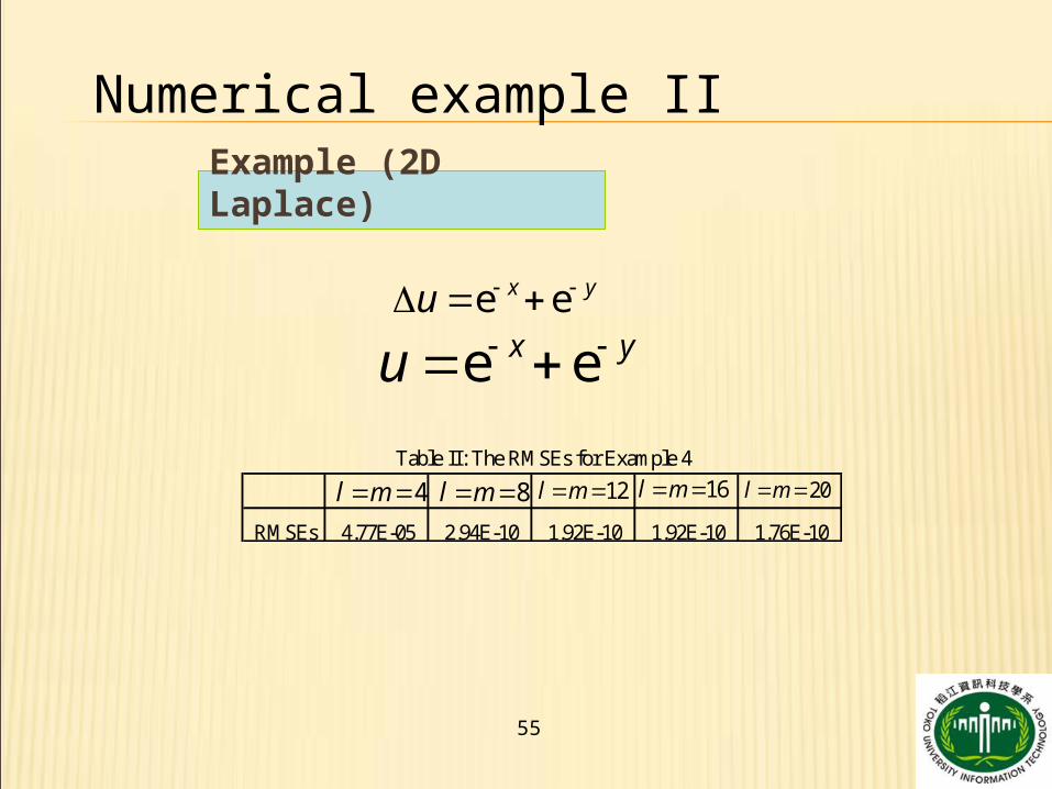
Example (2D Laplace)
e ex yu e ex yu
RMSEs 4.77E-05 2.94E-10 1.92E-10 1.92E-10 1.76E-10
Table II: The RMSEs for Example 4
4l m 8l m 12l m 16l m 20l m
Numerical example II
56
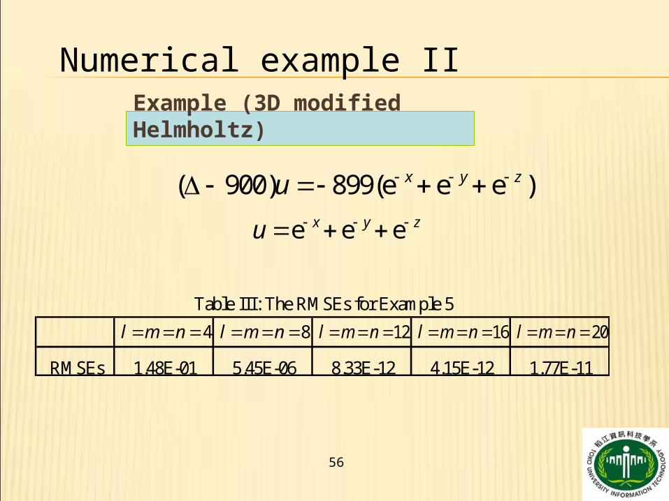
Example (3D modified Helmholtz)
( 900) 899(e e e )x y zu
e e ex y zu
RMSEs 1.48E-01 5.45E-06 8.33E-12 4.15E-12 1.77E-11
Table III: The RMSEs for Example 5
4l m n 8l m n 12l m n 16l m n 20l m n
Numerical example II
57
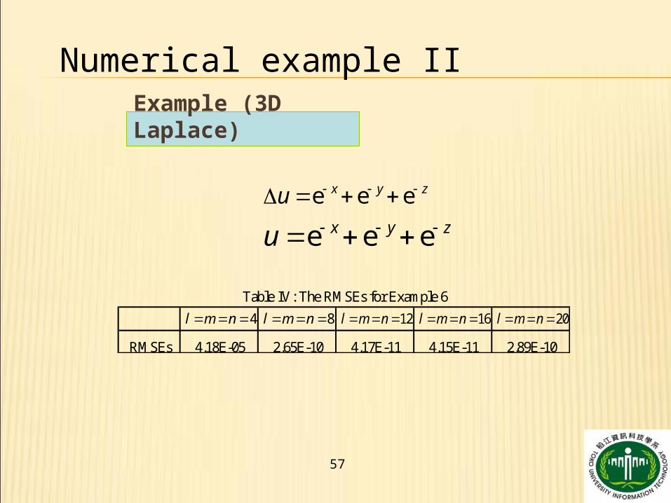
Example (3D Laplace)
e e ex y zu
e e ex y zu
RMSEs 4.18E-05 2.65E-10 4.17E-11 4.15E-11 2.89E-10
Table IV: The RMSEs for Example 6
4l m n 8l m n 12l m n 16l m n 20l m n
Numerical example II
58
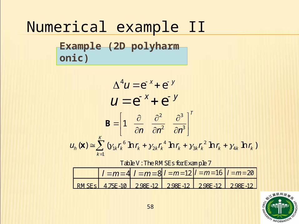
Example (2D polyharmonic)
e ex yu 4 e ex yu
2 3
2 31
T
n n n
B
RMSEs 4.75E-10 2.98E-12 2.98E-12 2.98E-12 2.98E-12
Table V: The RMSEs for Example 7
4l m 8l m 12l m 16l m 20l m
6 4 21 2 3 4
1
( ) ( ln ln ln ln )K
h k k k k k k k k k k kk
u r r r r r r r
x
Numerical example II
59
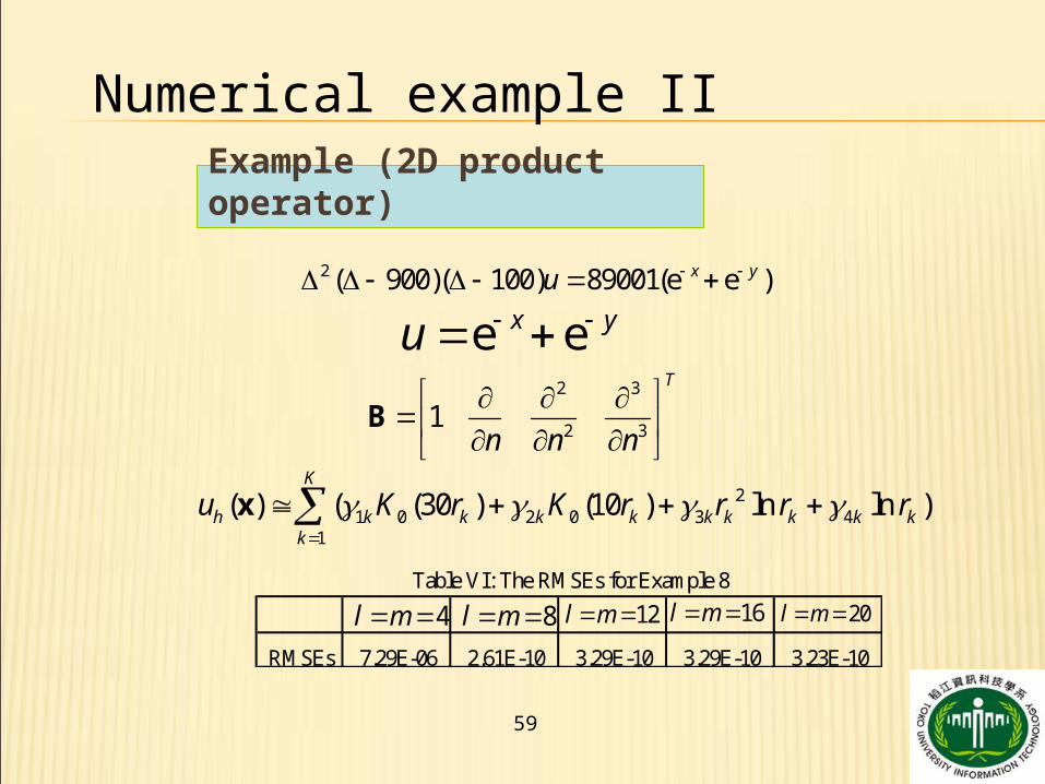
Example (2D product operator)
e ex yu 2 3
2 31
T
n n n
B
2 ( 900)( 100) 89001(e e )x yu
21 0 2 0 3 4
1
( ) ( (30 ) (10 ) ln ln )K
h k k k k k k k k kk
u K r K r r r r
x
RMSEs 7.29E-06 2.61E-10 3.29E-10 3.29E-10 3.23E-10
Table VI: The RMSEs for Example 8
4l m 8l m 12l m 16l m 20l m
Numerical example II
60
1. MFS+APS => scattered data in right-hand sides
2. MFS+Chebyshev => spectral convergence
3. Hörmander operator decomposition technique
4. Partial fraction decomposition
5. polyHelmholtz & Polyharmonic particular solutions
6. MFS for the product operator
Conclusion

61
Thank you